
Herbivory by Geese Inhibits Tidal Freshwater Wetland Restoration Success


1
Biological Sciences Department, George Washington University, Washington, DC 20052, USA
2
National Park Service, National Capital Parks-East, Washington, DC 20020, USA
*
Author to whom correspondence should be addressed.
Diversity 2022, 14(4), 278; https://0-doi-org.brum.beds.ac.uk/10.3390/d14040278
Submission received: 5 March 2022
/
Revised: 24 March 2022
/
Accepted: 29 March 2022
/
Published: 7 April 2022
/
Corrected: 25 October 2023
(This article belongs to the Special Issue Conservation and Ecological Restoration of Intertidal Marshes)
Abstract
:Experimental results from a multi-year exclosure study (2009–2015) demonstrate strong effects of geese on plant cover and species diversity in an urban, restored tidal freshwater wetland. Access by geese inhibited plant establishment and suppressed plant diversity, particularly of annual plant species. Our experimental results demonstrate that the protection of newly restored tidal freshwater wetlands from geese is a make-or-break management activity that will determine the composition and long-term persistence of vegetation at the site. The causal herbivore, in this case, was resident, non-migratory Canada geese (Branta canadensis), which have increased dramatically over the last several decades and had high population densities throughout the study period. These findings suggest that management activities to reduce the population sizes of non-migratory goose populations will support greater wetland plant diversity.
1. Introduction
Ecosystem restorations of tidal freshwater wetlands offer opportunities to probe and reveal the ecological processes structuring these systems, while also increasing the area of an imperiled habitat and providing ecosystem services. In this paper, we present some of the lessons learned from a tidal freshwater wetland (hereafter, TFW) restoration in the highly urbanized setting of the Anacostia River in Washington D.C., USA, where the authors and partner agencies conducted an experimental manipulation of goose herbivory to test the role of top-down effects on plant establishment and community composition [1,2].
Strong top-down effects can influence the success of a restoration project [3,4,5]. Of particular concern for tidal freshwater wetlands is the impact that Canada goose (Branta canadensis) herbivory plays in restoration efforts. Migratory goose populations have had an extensive impact on TFW, dramatically reducing the abundance of annual wild rice (Zizania aquatica) in existing TFW [6]. The population sizes of resident, non-migratory Canada geese grew exponentially throughout the 1980s and 1990s in the eastern United States [7,8]. In 2012, the number of resident, non-migratory geese in North America surpassed the number of migratory individuals [7]. Resident goose populations have been shown to impact plant communities present in TFWs and to have their greatest effect on annual plant species [9,10]. Problems with resident geese are likely to persist into the future; due to low adult mortality and favorable habitat conditions for breeding, current resident goose flocks are able to double in size every five years [11]. This highlights the need to better understand the role geese play in the success of TFW restoration projects to inform future efforts.
Located in the upper regions of estuaries [12], tidal freshwater wetlands often have been displaced by development and have experienced some of the greatest losses of any coastal habitat [13,14]. Large quantities of TFW were converted into agricultural fields and industrial development by infilling [15,16,17]. Common “head-of-tide” tidal restrictions suggest elimination of this habitat along many tidal rivers and creeks [18,19].
To reduce and mitigate these habitat losses, TFWs have been the subject of restoration efforts [20]. Urban wetlands can have a greater societal benefit than those in rural regions, due to the present scarcity of wetlands in densely populated areas, as well as the larger populations that can benefit from the ecosystem services produced by wetlands [21]. These ecosystem services include water infiltration, climate regulation, air purification, human health benefits, and recreational opportunities [22]. The high societal value of urban wetlands has led to renewed interest in urban restoration and a higher priority being placed on restoration projects in urban landscapes [23].
The methods used to restore TFW vary considerably [20]. Restoration of TFW on the East Coast of the United States often involves excavation of upland soils or placement of dredged materials in open water regions to create platforms for plant growth [16]. The beneficial use of dredged material is sometimes a motivation and an opportunity for TFW wetland restoration [24,25].
Our study site of Kingman Marsh is a 13-ha TFW restoration site located in Anacostia Park within Washington D.C., USA. The site was subject to dredging, seawalls, and tide gates that destroyed TFW habitat in the 1950s [26]. Restoration efforts began in 1999 by the U.S. Army Corps of Engineers (USACE), when dredged sediment was placed on site. In 2000, planted and volunteer vegetation was established at the site. However, in 2001, vegetation sampling conducted by the U.S. Geological Survey (USGS), the University of Maryland (UMD, College Park, MD, USA), and the National Park Service (NPS) documented the decimation of vegetation by herbivores, following the removal of fencing around plantings [27]. Herbivory appeared to limit restored areas from revegetating. The current study was initially designed by USGS in collaboration with NPS to document the impacts of herbivory, suspected to be by resident, non-migratory Canada geese. In this paper, researchers with George Washington University (Washington, DC, USA) provide the results of new analyses that enhance and build on the earlier USGS work.
2. Materials and Methods
2.1. Study Site
Kingman Marsh (latitude and longitude: 38°54′19.75″ N, 76°57′39.9″ W) is one of four TFW sites along the Anacostia River that were restored between 1993 and 2006 when the U.S. Army Corps of Engineers (USACE) began placing dredged sediment as a foundation for wetland plants. Kingman Marsh was the second site to be restored, after Kenilworth Marsh. Two additional sites, one along the mainstem of the Anacostia and one adjacent to nearby Heritage Island, were restored after Kingman, creating a network of restored TFWs of different ages in this stretch of the Anacostia River. Sediment for the Kingman Marsh restoration was placed by the USACE in the early 2000′s to create 13 ha of TFW, after which 750,000 plants of 7 perennial species (Supplementary of Table S1) were planted in May 2000. Most restored areas were surrounded by goose fences that were removed in the following winter, based on the initial success of the nearby unprotected TFW restoration at Kenilworth Marsh [27]. When fencing was removed at the Kingman Marsh site, goose herbivory on the newly established vegetation was extensive.
Kingman Marsh is surrounded by the Langston Golf Course (Figure 1). Through the center of the marsh is a slow-moving, shallow tidal creek that drains almost completely at low tide. To discourage dominance by the invasive common reed (Phragmites australis) and purple loosestrife (Lythrum salicaria), the sediment elevation contours at the site were set slightly lower than those of the Kenilworth Marsh restoration, where particularly P. australis had become problematic at higher elevations [27]. While the invasive species P. australis and L. salicaria are present at the Kingman Marsh site, they have not become the dominant species at the elevation of the experiment in Kingman Marsh, although P. australis has become dominant at higher elevations and has been subject to herbicide control activities in nonexperimental areas of the study site. For more information about the site and the network of restored marshes, see published reports and reviews [1,2,20,25,27].
2.2. Exclosure Experiment
Sixteen experimental modules were installed in Kingman Marsh in May 2009 (Figure 1) [1,2]. Module locations were selected from points that fell within an elevation range considered suitable for establishment of native emergent vegetation, 0.25 to 0.37 m above sea level (m.a.s.l.) relative to the North American Vertical Datum 1988 (NAVD88) [2]. Eight of the modules were located in areas with existing vegetation at the beginning of the experiment, due to their location within pre-existing fencing and seeding efforts by the Anacostia Watershed Society, and eight were within unvegetated areas (Figure 1). Modules were located at a minimum of 6 m apart.
Each module consisted of a pair of plots measuring 1 × 2 m. Plot corners were marked with PVC poles. Within each pair, one plot was randomly assigned to the exclosure treatment and one to an unfenced control. Paired plots were separated by a distance of 3 m. Exclosures were constructed out of steel t-posts surrounded by fencing 1.2 m tall, with a mesh size of 5 × 10 cm. Exclosures were 3 × 4 m to include a 1 m buffer surrounding the study plot, which limited disturbance by researchers entering the exclosure during data collection. Exclosures were open at the top, where taut string and flagging were placed to deter aerial access. A gap was left between the bottom of the fencing and the sediment surface to allow entry of animals other than geese. Initially, this gap was 20 cm high, but after video footage confirmed that geese could enter this small space, the gap was narrowed to 15 cm in 2010 and further narrowed to 10 cm in 2011 to prevent entry by geese. Exclosures were maintained every spring in March or April to ensure fencing was intact and at the correct height above the substrate for the start of the growing season.
Plant community composition and abundance was monitored each June and August beginning in 2009. A 1 × 2 m PVC frame with a 25 × 25 cm grid was placed over plots and the cover of each plant species present in the plot was estimated independently. Estimates were made to the nearest 1% between 0–15% and 95–100%, because in these ranges it is straightforward to accurately estimate cover. Between 15 and 95% cover, estimates were made in 5% increments. Taxonomic nomenclature follows the ITIS online database [28]. Whenever possible, two researchers made independent estimates of each species and determined a final visual estimate by consensus. Total vegetative cover was calculated as the sum of the cover values for all of the taxa. Since species often overlap within the emergent herbaceous layer, the total vegetative cover frequently exceeded 100%. Along with cover of plant taxa, the percent cover of bare area (no plant cover) and detritus (dead, detached plant material) were also estimated.
Plant identifications were done visually, using known plant characteristics. When species could not be identified in the field, a specimen of the same morphospecies from outside the plot was collected, and the fresh sample was identified in the laboratory using a microscope and Flora of Virginia [29] as a primary reference and the PLANTS online database [30] as a secondary reference.
2.3. Goose Population Census
Each summer, in July 2009 and early to mid-June of each subsequent year, non-migratory Canada geese were surveyed at 30 sampling stations located around the network of Anacostia TFW restoration sites. The seasonal timing of the goose survey coincided with nesting and sedentary behavior, so that geese were less likely to take flight and more likely to be included within the count. At low tide on four to six subsequent days, observers counted goslings and adult geese across the network of TFW, with each observer assigned designated stations that were repeatedly sampled each year. The mean daily total across all sites was used as an estimate of the resident goose population, and the standard error of the estimate was calculated as the standard deviation of all days around the mean divided by the number of days of sampling.
2.4. Statistical Analyses
Analyses were done in R [31]. August data was used to assess interannual change. Monitoring data from June 2009 was used as a pre-experimental baseline. For each plot, we calculated total vegetative cover by summing each species’ percent cover, excluding bare ground and detritus. We also explicitly investigated the contribution of annual species to the total percent cover. We calculated species richness and Shannon–Wiener Diversity Index using the package ‘vegan’ [32]. For total vegetative cover, cover of annual species, species richness, and Shannon-Wiener Diversity Index, differences between paired fenced and unfenced control plots were calculated and analyzed using a mixed model for repeated measures, using the package ‘nlme’ [33] to compare data among years (2009–2015) and initial vegetation states (initially vegetated or initially unvegetated) and their interactions. This statistical approach was developed by J. Hatfield at the USGS [1,2]. All four response variables were transformed prior to analysis using a natural log transformation to improve normality. We performed the log transformation by taking the difference in logs since the difference between fenced and unfenced control plots was sometimes negative. Pairwise comparisons were made using Tukey’s Studentized Test of Least Squares Means to detect whether fenced–unfenced control differences varied over time and initial vegetation state. Then, three variance–covariance structures were modeled (compound symmetry, autoregressive, and unstructured), and the best model was selected using AIC comparisons to describe the independent and interactive effects of exclosure treatment, initial vegetation state, and time. Inspection of least square means and associated t-tests with Bonferroni adjusted p-values for multiple comparisons were used to determine the significance of the exclosure treatment.
To examine the species composition data, we used non-metric multidimensional scaling (NMDS) with Bray–Curtis dissimilarity in the ‘vegan’ package to generate an ordination of the community composition. We graphed the group centroids of the four different treatments (exclosure × initial vegetation state) through time, with individual plot points in the background. To analyze the relationship between year, initial vegetation state, and exclosure treatment on community composition, we performed a Permutational Multivariate Analysis of Variance (PERMANOVA).
3. Results
3.1. Exclosure Experiment
3.1.1. Vegetative and Annuals Cover
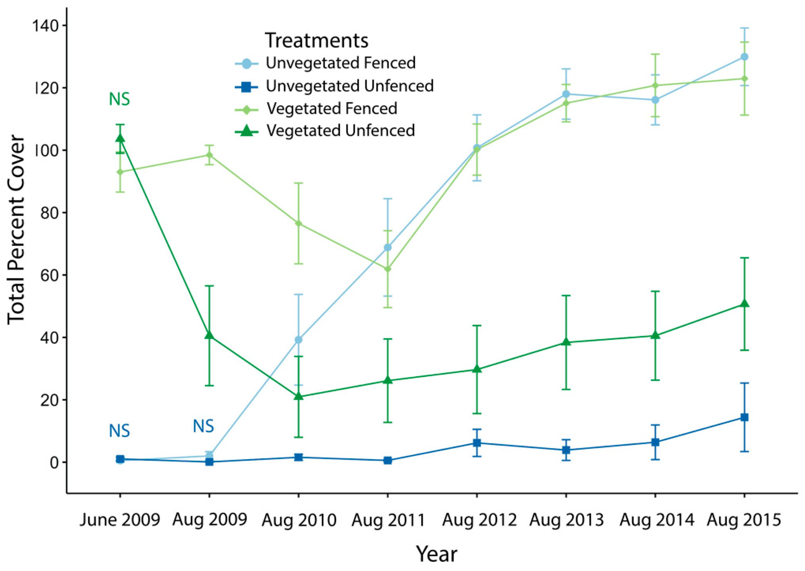
In the start of the study in June 2009, there was no difference in total vegetative cover between fenced and unfenced plots (initially vegetated: fenced 93.0 ± 6.4% vs. unfenced 103.6 ± 4.6%, t(7) = 1.30, p = 0.23; initially unvegetated: fenced 1.0 ± 0.6% vs. unfenced 0.5 ± 0.4%, t(7) = 0.894, p = 0.40; all p-values for t-tests represent Bonferroni-adjusted p-values, Table S2). By August 2009, in the initially vegetated plots, there was a significant effect of exclosures with fenced plots having more than double the percent cover of unfenced plots (fenced 98.5 ± 3.1% vs. unfenced 40.5 ± 16%, t(7) = −3.43, p = 0.01). Whereas, for the initially unvegetated plots, a significant exclosure effect did not occur until the following year in August 2010 (fenced 39.3 ± 14.5% vs. unfenced 1.6 ± 1%, t(7) = −2.69, p = 0.03). After 2010, the effect persisted in every year of the experiment, with fenced plots producing greater total vegetative cover than paired unfenced plots (Figure 2).
The mixed model for repeated measures utilized an autoregressive variance-covariance structure selected based on AIC comparisons to investigate the difference between the percent cover for the fenced and the paired unfenced control (Table 1). We found a significant interaction between initial vegetation state and year of study (= 2.80; p = 0.01, Table 1). The post-hoc comparison contrasted the exclosure effect in initially vegetated plots vs. initially unvegetated plots across all years. The exclosure effect (difference between fenced and unfenced control plots) began to diverge in initially vegetated and initially unvegetated modules beginning in 2013 (t(42) = 2.348, p = 0.02) and continued to persist the following two years (2014: (t(52) = 3.383, p = 0.001); 2015 (t(34) = 2.315, p = 0.03). Exclosures had a similar impact on initially vegetated and unvegetated plots for the first four years, until the rate at which percent cover began to asymptote in vegetated plots due to their high initial starting point and the additional vegetative growth in exclosures reaching a maximum. Additionally, several of the vegetated modules began with a higher cover of Peltandra virginica, an unpalatable, native, perennial species, leading to more persistent vegetation in unfenced plots that were initially vegetated than those that were initially unvegetated (Figure 1). Whereas, in the later years of the study, the unvegetated plots had a greater remaining capacity for differences between the fenced and unfenced plots, due to the lack of vegetation at the time of exclosure.
In nearly all surveys following the collection of baseline data in June 2009, cover of annual species was significantly greater in fenced plots than unfenced plots (Table S2). In the repeated measures mixed model, similar to total percent cover, there was a significant interaction effect between initial vegetation and year of study on the difference in percent cover of annuals between fenced and unfenced treatments (= 2.85; p = 0.01, Table 1). This was due to a single year, 2011, when the difference in annual cover between fenced and unfenced plots was smaller in initially vegetated plots than initially unvegetated plots. Generally, the percent cover of annuals in fenced plots of initially vegetated modules started very high and declined in the first year of the study, whereas it started very low in initially unvegetated modules and increased in fenced plots during the first year to converge on the same range in fenced plots of all types (Figure 3). Throughout the subsequent years, other than the dip in 2011 in fenced initially vegetated plots, the percent of annuals in all fenced plots stabilized at about 30% cover and remained very low (near 0%) for unfenced plots (Figure 3).
3.1.2. Diversity Measures
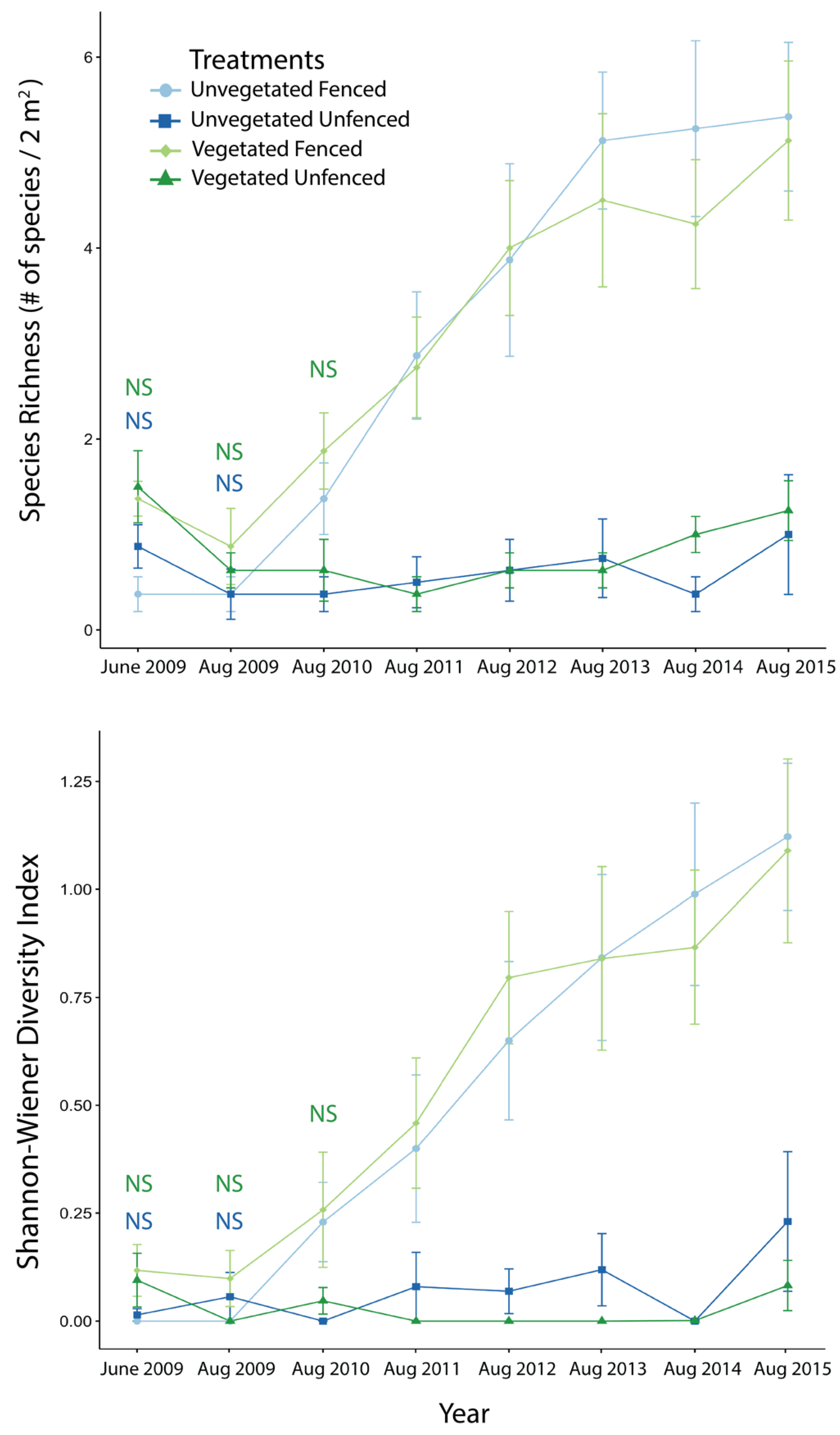
At the beginning of the study, fenced and unfenced plots within each of the initial vegetation states were similar in diversity, in both diversity metrics of species richness and the Shannon–Wiener Diversity Index (Table S2). Differences between fenced and unfenced plots in diversity began to emerge in 2010, when fenced treatments within initially unvegetated plots showed significantly higher species richness and diversity than unfenced plots (Richness: t(7) = −2.65, p = 0.033; Shannon Wiener Diversity Index: t(7) = −2.50, p = 0.041). Exclosure treatments within initially vegetated plots began to show the same effect in 2011 (Richness: t(7) = −4.46, p = 0.003; Shannon–Wiener Diversity Index: t(7) = −3.04, p = 0.019). Differences between fenced and unfenced plots remained and grew in magnitude throughout the remainder of the experiment (Figure 4).
Similar to the vegetative cover mixed model, the best model (i.e., lowest AIC) for describing the effects of initial vegetation state, exclosure treatment, and time on diversity was a mixed model for repeated measures with an autoregressive variance-covariance structure. In this model, only year significantly affected species richness (= 13.59; p = 0.0001) and diversity (= 12.31; p = 0.0001). The difference between fenced and unfenced plots steadily increased through time for species richness and diversity. Unlike the pairwise comparisons, this model suggested that unfenced plots had a slightly greater species richness than fenced plots at the start of the experiment in 2009. However, over the course of the experiment, species richness became much greater in fenced plots compared to unfenced control plots (by an estimated 1.16 ± 0.14 species). For diversity, there was no initial difference between fenced and unfenced plots (mean of 0.003 ± 0.033); by 2015, this difference had increased to 0.59 ± 0.07.
3.1.3. Community Composition
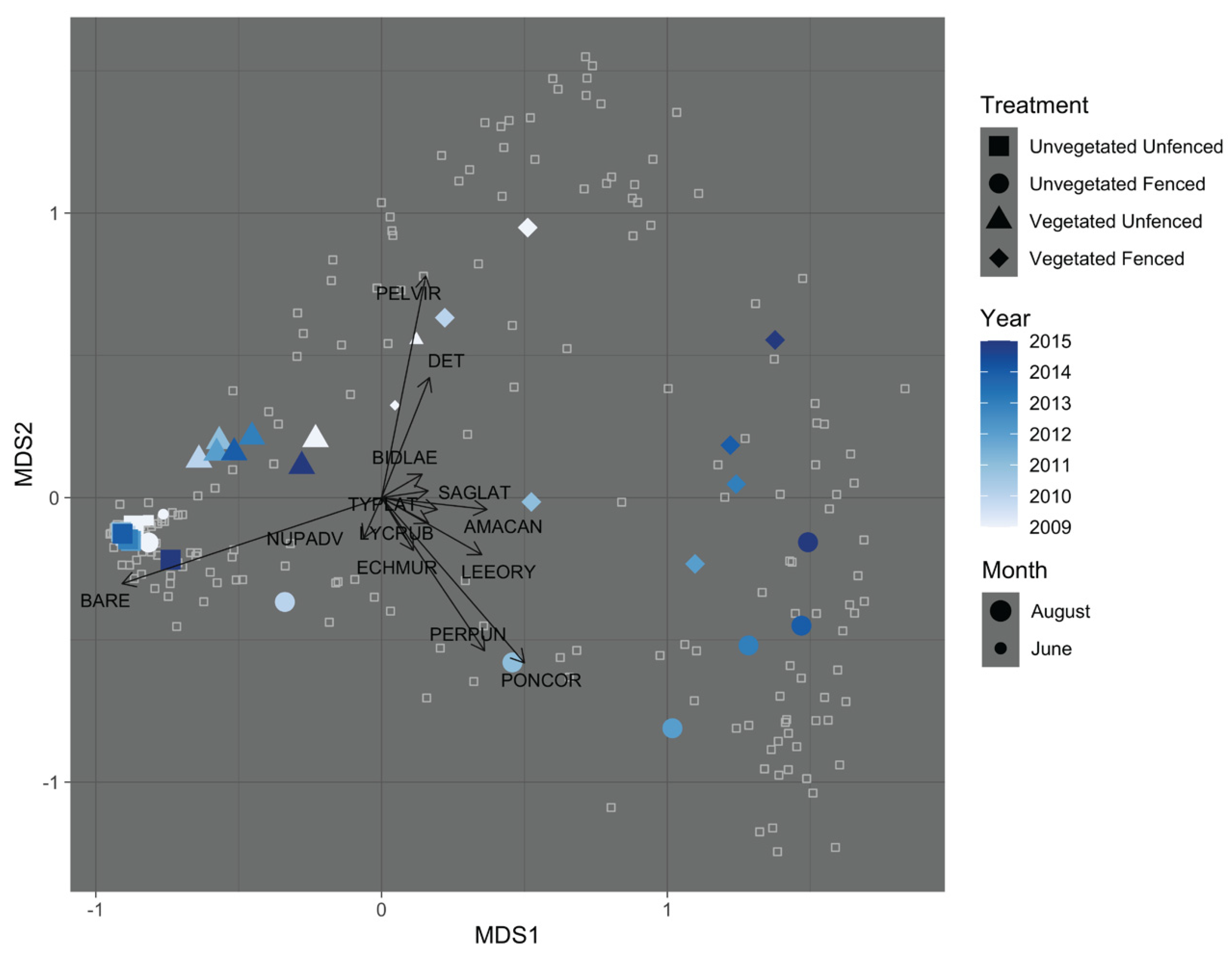
Ordination by non-metric multidimensional scaling (NMDS) produced a simplified description of community composition (three dimensions, stress = 0.094 after 170 iterations). The ordination shows differences in community composition between the exclosure treatments that grow through time and that differ by initial vegetation state (Figure 5). In ordination, it is easy to see the similarity between fenced and unfenced unvegetated communities in June 2009, as well as fenced and unfenced vegetated communities. Over time, fenced treatments of both initial vegetation states separate from unfenced treatments, whereas plant communities of both initial vegetation states in unfenced plots remained in a relatively confined and tight ordination space through time, indicating little change in community composition over time for unfenced treatments throughout the study. Permutational Multivariate Analysis of Variance (PERMANOVA) revealed a significant three-way interaction between fencing treatment, initial vegetation, and year (= 4.20; p = 0.01). In PERMANOVA, the largest proportion of the variation in plant community composition was explained by exclosure treatment ( = 0.189) and secondarily by initial vegetation state ( = 0.075). Time ( = 0.056), and the interaction of exclosure treatment and time ( = 0.058) explained smaller amounts of variation in community composition. The three-way interaction of exclosure treatment, initial vegetation state, and time explained very little variation in the NMDS ordination ( = 0.009). The species that contributed most to these compositional changes (Pontederia cordata, Peltandra virginica, Persicaria punctata, and Leersia oryzoides) are depicted by the longest species vectors in Figure 5.
3.2. Goose Population Census
During the study period, the counted goose population was relatively large. It ranged from a minimum of 402 individuals in 2010 to a maximum of 654 individuals in 2012 (Figure 6). The population increased between 2010 and 2012, but from 2012 to 2015, population levels returned to the level observed during the first years of study.
4. Discussion
At the restored tidal freshwater wetland at Kingman Marsh, plant communities exposed to herbivory by resident, non-migratory Canada geese are vastly different than communities protected from this top-down pressure. When these plant communities were protected in exclosures, total percent cover, percent cover of annuals, species richness, and diversity all increased compared to a paired, unfenced control plot. These differences occurred rather rapidly, within the first 2 years of the study, and remained consistent or increased through time. Not only did plant cover and diversity increase once herbivory was excluded, but the overall community composition shifted in response to the fencing treatment, becoming significantly distinct from the plant communities left unprotected, which hardly changed at all through the study period (Figure 5). These results highlight the striking effects that goose herbivory can have on TFW plant communities, especially in an urban restoration context, and the importance of considering the role of top-down forces in restoration success.
Often, restoration efforts target only historical abiotic conditions of the system, neglecting the role of biotic factors in restoration success [34] and the unexpected outcomes that can result when biotic factors are neglected [35]. In the case of Kingman Marsh, the impact of herbivory was underestimated for the nascent restoration project based on the initial success at the nearby unprotected Kenilworth Marsh restoration and fences were removed, with the outcome that the site was subsequently significantly denuded [27].
Other studies have also found resident Canada geese to play a significant role in TFW plant communities. However these studies have primarily focused on the impacts on a single plant species, annual wild rice (Zizania aquatica), and have been conducted in more rural or suburban contexts [6,10]. To our knowledge, no previous study has investigated the impact of resident geese on restoration success in an urban setting or investigated the effects holistically on the entire TFW plant community.
Our study did not just evaluate the effect of goose herbivory on the TFW plant community; it also looked at the effect of the starting point of the plant community on the effect of herbivory. In initially unvegetated plots, it took an extra year of recovery inside exclosures to observe the effect of herbivory on total percent cover and percent cover of annuals. However, the overall differences between initially unvegetated and initially vegetated modules were small. For example, in species richness and diversity, the initial vegetation state made no difference; diversity within exclosures climbed through time, whereas outside of exclosures, diversity remained very low (Figure 4). In community composition, as well, the effect of the initial vegetation state was small relative to the effect of the exclosure treatment.
When geese were excluded from the community, we observed high levels of vegetative cover and a preferred mix of annual and perennial species cover. Annual species are an important and unique component of TFW, in that their overall biomass is relatively stable year-to-year, even as species composition can be quite variable [36]. Leck and Crain [37] suggest a target for annual species cover in restored TFW that is between 20 and 50% cover. The cover of annuals in the experimental exclosures met this criterion within the second year of the experiment, and levels of annual cover remained relatively stable throughout the study. The high proportion of annuals in fenced plots suggests that, even in this urban setting, the seed bank is a resilient source of annual and perennial species that will promote high biodiversity, if only herbivory by geese can be kept in check.
Urban wetland restoration is a challenge because most sites are heavily degraded and multi-use is an important restoration goal that, preferably, can co-exist with ecological targets [38]. Also, urban wetlands are often geographically isolated from other wetland habitats by urban land use [39]. The isolated nature of urban wetlands may concentrate herbivore pressure and make urban wetlands particularly vulnerable to the impacts of goose herbivory. At the same time, resident geese are more rapidly increasing in urban and exurban areas due to the prevalence of lawns and stormwater infrastructure, and in this case, a golf course, as well as a relative paucity of predators and difficulty of implementing a hunting program [40]. In more rural regions, land and waterfowl managers can utilize early season control efforts that specifically target resident geese prior to the arrival of migratory individuals [10]. This is more difficult in an urban setting, since most cities have local ordinances prohibiting firearm discharges [41]. As urban wetlands do not have the benefit of utilizing hunting to reduce resident goose populations, there are fewer management options [42]. Effectively managing resident goose populations in urban areas can be especially challenging.
The impact of resident, non-migratory Canada geese on restoration success at Kingman Marsh, reported here, revealed the need to effectively control their population within the restored TFW of the Anacostia River in order to meet vegetation recovery targets and to support the high plant biodiversity typical of TFW communities. These experimental results were the impetus for the resident goose population control efforts (oiling eggs and cull roundups) directed by the National Park Service beginning in 2018. Since 2015, surveys of these modules and goose populations have continued and another unpalatable species, Nuphar advena, has increased in abundance (see the species established in 2015 in the photo in Figure 1B), results which will be reported in a subsequent article. We expect the differences between fenced and unfenced plots to decrease in magnitude and possibly disappear when the top-down control by resident geese is kept in check by population control measures.
The restoration practices presented here represent a case of adaptive management. The initial restoration activities of sediment placement have been successful in creating TFW habitats but have not met vegetation cover or biodiversity targets. Based on our findings, the level of goose herbivory was identified as the factor limiting development of this ecosystem and is now the focus of restoration efforts in the Anacostia River TFW network. The collaboration between agencies and institutions involved in the restoration of Anacostia River TFW has provided the monitoring and expertise necessary to make informed decisions in the adaptive management plan. The history of this site reiterates that continued monitoring and adaptive management are integral to positive restoration outcomes.
5. Conclusions
An exclosure experiment in an urban, restored, tidal freshwater wetland revealed the important role of resident, non-migratory Canada geese in vegetation establishment and community composition. Plant diversity, vegetative cover, and the proportion of annual plant species were reduced by goose herbivory. In the absence of goose herbivory, in exclosures, these metrics recovered quickly, in two growing seasons, and to levels considered acceptable and desirable in other restoration projects and contexts. Although the urban environment is a challenging context in which to manage resident Canada goose populations, goose control is necessary for restoration success in tidal freshwater wetlands.
Supplementary Materials
The following supporting information can be downloaded at: https://0-www-mdpi-com.brum.beds.ac.uk/1424-2818/14/4/278/s1, Table S1 lists all plant species identified in the study plots. Table S2 details paired t-test statistics for comparisons between years of differences between fenced and unfenced plots.
Author Contributions
Conceptualization: C.K. and M.M.; methodology and data collection: C.K. and M.M.; data curation: C.K.; formal analysis: J.J.; writing—original draft preparation: J.J. and K.G.; writing—review and editing: all; supervision and project administration: K.G.; funding acquisition: C.K., M.M., and K.G. All authors have read and agreed to the published version of the manuscript.
Funding
This research was funded by NSF Graduate Research Fellowship award number 1746914 awarded to J. Jobe. The Chesapeake Watershed Cooperative Ecosystem Studies Unit Master Cooperative Agreement P17AC01377 supported this collaboration between the National Park Service and George Washington University.
Institutional Review Board Statement
Not applicable.
Data Availability Statement
The data presented in this study will be openly available on GitHub.
Acknowledgments
We would like to acknowledge some key collaborators on the project: Richard Hammerschlag (USGS), who helped to install and monitor the experiment, Glenn Guntenspergen (USGS), who helped to design the experiment, and Jeff Hatfield (USGS), who helped design the statistical analysis and provided analytical support. A variety of agencies and partners have contributed to restoration work on Anacostia over the years, through engineering design and implementation, managing authority, financial support, personnel for monitoring vegetation and Canada geese, and supplemental plantings. Contributors have included the United States Army Corps of Engineers, National Park Service, United States Geological Survey, University of Maryland, Washington D.C.’s Department of Energy and the Environment (formerly District Department of the Environment), and the Anacostia Watershed Society.
Conflicts of Interest
The authors declare no conflict of interest. The funders had no role in the design of the study; in the collection, analyses, or interpretation of data; in the writing of the manuscript, or in the decision to publish the results.
References
- Krafft, C.C.; Hatfield, J.S.; Hammerschlag, R.S. Effects of Canada Goose Herbivory on the Tidal Freshwater Wetlands in Anacostia Park, 2009–2011; National Park Service: Washington, DC, USA, 2013.
- Krafft, C.C.; Hatfield, J.S.; Hammerschlag, R.S. Effects of Canada Goose Herbivory on the Tidal Freshwater Wetlands in Anacostia Park, 2009–2015; National Park Service: Washington, DC, USA, 2015.
- Sweeney, B.W.; Czapka, S.J.; Yerkes, T. Riparian Forest Restoration: Increasing Success by Reducing Plant Competition and Herbivory. Restor. Ecol. 2002, 10, 392–400. [Google Scholar] [CrossRef]
- Thyroff, E.C.; Burney, O.T.; Jacobs, D.F. Herbivory and Competing Vegetation Interact as Site Limiting Factors in Maritime Forest Restoration. Forests 2019, 10, 950. [Google Scholar] [CrossRef]
- Wasson, K.; Tanner, K.E.; Woofolk, A.; McCain, S.; Suraci, J.P. Top-down and Sideways: Herbivory and Cross-Ecosystem Connectivity Shape Restoration Success at the Salt Marsh-Upland Ecotone. PLoS ONE 2021, 16, e0247374. [Google Scholar] [CrossRef] [PubMed]
- Nichols, T.C. Ten Years of Resident Canada Goose Damage Management in a New Jersey Tidal Freshwater Wetland. Wildl. Soc. Bull. 2014, 38, 221–228. [Google Scholar] [CrossRef]
- Dolbeer, R.A.; Seubert, J.L.; Begier, M.J. Population Trends of Resident and Migratory Canada Geese in Relation to Strikes with Civil Aircraft. Hum.-Wildl. Interact. 2014, 8, 88–99. [Google Scholar]
- Conover, M.R. Population Growth and Movements of Canada Geese in New Haven County, Connecticut, during a 25-Year Period. Waterbirds Int. J. Waterbird Biol. 2011, 34, 412–421. [Google Scholar] [CrossRef]
- Baldwin, A.H.; Pendleton, F.N. Interactive Effects of Animal Disturbance and Elevation on Vegetation of a Tidal Freshwater Marsh. Estuaries 2003, 26, 905–915. [Google Scholar] [CrossRef]
- Haramis, G.M.; Kearns, G.D. Herbivory by Resident Geese: The Loss and Recovery of Wild Rice along the Tidal Patuxent River. J. Wildl. Manag. 2007, 71, 788–794. [Google Scholar] [CrossRef]
- Smith, A.E.; Craven, S.R.; Curtis, P.D. Managing Canada Geese in Urban Environments; Cornell Cooperative Extension: Ithaca, NY, USA, 2000. [Google Scholar]
- Simpson, R.L.; Good, R.E.; Leck, M.A.; Whigham, D.F. The Ecology of Freshwater Tidal Wetlands. BioScience 1983, 33, 255–259. [Google Scholar] [CrossRef]
- Ehrenfeld, J.G. Evaluating Wetlands within an Urban Context. Urban Ecosyst. 2000, 4, 69–85. [Google Scholar] [CrossRef]
- Whigham, D.F.; Baldwin, A.H.; Swarth, C. Conservation of Tidal Freshwater Wetlands in North America. In Tidal Freshwater Wetlands; Elsevier: Amsterdam, The Netherlands, 2009. [Google Scholar]
- Baden, J., III; Batson, W.T.; Stalter, R. Factors Affecting the Distribution of Vegetation of Abandoned Rice Fields, Georgetown Co., South Carolina. Castanea 1975, 40, 171–184. [Google Scholar]
- Baldwin, A.H.; Barendregt, A.; Whigham, D.F. Tidal Freshwater Wetlands, an Introduction to the Ecosystem. In Tidal Freshwater Wetlands; Elsevier: Amsterdam, The Netherlands, 2009. [Google Scholar]
- Swarth, C.W.; Delgado, P.; Whigham, D.F. Vegetation Dynamics in a Tidal Freshwater Wetland: A Long-Term Study at Differing Scales. Estuaries Coasts 2013, 36, 559–574. [Google Scholar] [CrossRef]
- Crain, C.M.; Gedan, K.B.; Dionne, M. Tidal Restrictions and Mosquito Ditching in New England Marshes. Human Impacts on Salt Marshes: A Global Perspective; University of California Press: Berkeley, CA, USA, 2009; pp. 149–169. [Google Scholar]
- Davidson, N.C. How Much Wetland Has the World Lost? Long-Term and Recent Trends in Global Wetland Area. Mar. Freshw. Res. 2014, 65, 934–941. [Google Scholar]
- Baldwin, A.H.; Hammerschlag, R.S.; Cahoon, D.R. Evaluating Restored Tidal Freshwater Wetlands. In Coastal Wetlands; Elsevier: Amsterdam, The Netherlands, 2019; pp. 889–912. [Google Scholar]
- Mazzotta, M.; Bousquin, J.; Berry, W.; Ojo, C.; McKinney, R.; Hyckha, K.; Druschke, C.G. Evaluating the Ecosystem Services and Benefits of Wetland Restoration by Use of the Rapid Benefit Indicators Approach. Integr. Environ. Assess. Manag. 2019, 15, 148–159. [Google Scholar]
- Collas, L.; Green, R.E.; Ross, A.; Wastell, J.H.; Balmford, A. Urban Development, Land Sharing and Land Sparing: The Importance of Considering Restoration. J. Appl. Ecol. 2017, 54, 1865–1873. [Google Scholar] [CrossRef]
- Baldwin, A.H. Restoring Complex Vegetation in Urban Settings: The Case of Tidal Freshwater Marshes. Urban Ecosyst. 2004, 7, 125–137. [Google Scholar]
- Bowers, J.K. Innovations in Tidal Marsh Restoration: The Kenilworth Marsh Account. Restor. Manag. Notes 1995, 13, 155–161. [Google Scholar] [CrossRef]
- Neff, K.P.; Rusello, K.; Baldwin, A.H. Rapid Seed Bank Development in Restored Tidal Freshwater Wetlands. Restor. Ecol. 2009, 17, 539–548. [Google Scholar]
- Scott, P. Capital Engineers: The US Army Corps of Engineers in the Development of Washington, DC 1790–2004; Army Corps of Engineers Alexandria VA Office of History: Alexandria, VA, USA, 2011. [Google Scholar]
- Hammerschlag, R.S.; Baldwin, A.H.; Krafft, C.C.; Neff, K.P.; Paul, M.M.; Brittingham, K.D.; Rusello, K.; Hatfield, J.S. Five Years of Monitoring Reconstructed Freshwater Tidal Wetlands in the Urban Anacostia River (2000–2004); USGS: Reston, VA, USA, 2006.
- Hammerschlag, R.S.; Krafft, C.C. Five-Year Post-Reconstruction Kingman Marsh Monitoring Project: Vegetation; USGS: Reston, VA, USA, 2006.
- ITIS Integrated Taxonomic Information System 2015. Available online: www.itis.gov (accessed on 12 January 2022).
- Weakley, A.S.; Ludwig, J.C.; Townsend, J.F.; Crowder, B. Flora of Virginia; Botanical Research Institute of Texas Press: Fort Worth, TX, USA, 2012; ISBN 978-1-889878-38-6. [Google Scholar]
- USDA. The PLANTS Database 2015. National Plant Data Team: Greensboro, NC, USA. Available online: http://plants.usda.gov (accessed on 12 January 2022).
- R Core Team R: The R Project for Statistical Computing. Available online: https://www.r-project.org/ (accessed on 23 February 2022).
- Oksanen, J.; Blanchet, F.G.; Kindt, R.; Legendre, P.; Minchin, P.R.; O’Hara, R.B.; Simpson, G.L.; Solymos, P.; Stevens, M.H.H.; Wagner, H. Vegan: Community Ecology Package. R Package Version 2.0-10. 2013. 2015. Available online: https://CRAN.R-project.org/package=vegan (accessed on 23 February 2022).
- Pinheiro, J.; Bates, D.; DebRoy, S.; Sarkar, D.; Heisterkamp, S.; Van Willigen, B.; Maintainer, R. Package ‘Nlme.’ Linear Nonlinear Mixed Effects Models Version. 2017, Volume 3. Available online: https://cran.r-project.org/web/packages/nlme/index.html (accessed on 23 February 2022).
- Suding, K.N.; Gross, K.L.; Houseman, G.R. Alternative States and Positive Feedbacks in Restoration Ecology. Trends Ecol. Evol. 2004, 19, 46–53. [Google Scholar] [PubMed]
- Zedler, J.B. Progress in Wetland Restoration Ecology. Trends Ecol. Evol. 2000, 15, 402–407. [Google Scholar] [CrossRef]
- Whigham, D.F.; Simpson, R.L. Annual Variation in Biomass and Production of a Tidal Freshwater Wetland and Comparison with Other Wetland Systems. Va. J. Sci. 1992, 43, 5–14. [Google Scholar]
- Leck, M.A.; Crain, C.M. Northeastern North America Case Studies—New Jersey and New England. In Tidal Freshwater Wetlands; Elsevier: Amsterdam, The Netherlands, 2009; pp. 145–156. [Google Scholar]
- Zedler, J.B.; Leach, M.K. Managing Urban Wetlands for Multiple Use: Research, Restoration, and Recreation. Urban Ecosyst. 1998, 2, 189–204. [Google Scholar] [CrossRef]
- Callaway, J.C.; Zedler, J.B. Restoration of Urban Salt Marshes: Lessons from Southern California. Urban Ecosyst. 2004, 7, 107–124. [Google Scholar] [CrossRef]
- Balkcom, G.D. Demographic Parameters of Rural and Urban Adult Resident Canada Geese in Georgia. J. Wildl. Manag. 2010, 74, 120–123. [Google Scholar] [CrossRef]
- Holevinski, R.A.; Curtis, P.D.; Malecki, R.A. Hazing of Canada Geese Is Unlikely to Reduce Nuisance Populations in Urban and Suburban Communities. Hum. Wildl. Confl. 2007, 1, 257–264. [Google Scholar]
Figure 1.
(A) Satellite image of the site, Kingman Marsh, with points to show each module and an inset to show the location of the marsh in Washington D.C., USA. Photos show a fenced and unfenced pair of plots in (B), an initially unvegetated module (number 5 in (A)), (C) an initially vegetated module (number 11 in (A)). Photos were taken in August 2015. Plot corners are designated with white PVC pipes (partially obscured by vegetation in the initial vegetated module).

Figure 2.
Total percent cover through time in fenced (lighter colors) and unfenced (darker colors) plots of initially vegetated (green) and initially unvegetated (blue) modules. June 2009 data are included as a baseline; all other data presented were collected in August to reflect that year’s growing season. Labels of “NS” indicate a non-significant difference between control and exclosure treatments on that sampling date, color-coded to indicate initially vegetated state; on all other dates, differences were statistically significant. t-test statistics are reported in Table S2. Error bars are standard error.

Figure 3.
Percent cover of annual species through time in fenced (lighter colors) and unfenced (darker colors) plots of initially vegetated (green) and initially unvegetated (blue) modules. June 2009 data are included as a baseline; all other data presented were collected in August to reflect that year’s growing season. Labels of “NS” indicate a nonsignificant difference between control and exclosure treatments on that sampling date and color-coded to indicate initially vegetated state; on all other dates, differences were statistically significant. t-test statistics are reported in Table S2. Error bars are standard error.

Figure 4.
Species richness (top) and Shannon–Wiener Diversity Index (bottom) through time in fenced (lighter colors) and unfenced (darker colors) plots of initially vegetated (green) and initially unvegetated (blue) modules. June 2009 data are included as a baseline; all other data were collected in August to reflect that year’s growing season. Labels of “NS” indicate a non-significant difference between control and exclosure treatments for that sampling date, color-coded to indicate initially vegetated (green) or initially unvegetated (blue) modules; on all other dates, differences were statistically significant. T-test statistics are reported in Table S2. Error bars are standard error.

Figure 5.
Ordination of the vegetation plots by non-metric multidimensional scaling (NMDS). June data is only included in 2009, as baseline data; all other years are August only. The June 2009 symbols are smaller; the June 2009 symbol for the Unvegetated Unfenced treatment is slightly more difficult to identify but can be found in the cloud of points located in the far left of the plot. Colored centroids symbolize the average position across each treatment and year combination. Hollow squares represent community composition of an individual plot in a single year. Vectors describe the plant community compositional changes in plots. Vectors are included only for species that had a significant effect in NMDS (p < 0.05). Species vectors are coded with the first three letters of the genus and first three letters of the species name: AMACAN: Amaranthus cannabinus; BARE: Bare (no vegetation or detritus cover), BIDLAE: Bidens laevis; DET: Detritus; ECHMUR: Echinochloa muricata var. muricata; LEEORY: Leersia oryzoides; LYCRUB: Lycopus rubellus; NUPADV: Nuphar advena; PELVIR: Peltandra virginica; PERPUN: Persicaria punctata; PONCOR: Pontederia cordata; SAGLAT: Sagittaria latifolia; TYPLAT: Typha latifolia.

Figure 6.
Daily total count of resident, non-migratory geese in the Anacostia restored tidal wetlands censused in the years of 2009 to 2015. Error bars are standard error.
Figure 6.
Daily total count of resident, non-migratory geese in the Anacostia restored tidal wetlands censused in the years of 2009 to 2015. Error bars are standard error.


Table 1.
Repeated Measures ANOVA Results of the Effects of Initial Vegetation State and Year on the Difference in Total Percent Cover, Cover by Annual Species, Species Richness, and Shannon–Wiener Diversity Index between Fenced and Unfenced Treatments.
Table 1.
Repeated Measures ANOVA Results of the Effects of Initial Vegetation State and Year on the Difference in Total Percent Cover, Cover by Annual Species, Species Richness, and Shannon–Wiener Diversity Index between Fenced and Unfenced Treatments.
| Model Terms | Total Percent Cover | Cover by Annual Species | Species Richness | Shannon–Wiener Diversity Index | |||||
|---|---|---|---|---|---|---|---|---|---|
| d.f. | F | p | F | p | F | p | F | p | |
| Intercept | 1112 | 0.02 | 0.89 | 1.39 | 0.24 | 47.12 | <0.01 | 39.54 | <0.01 |
| Init. Vegetation | 1112 | 4.30 | 0.04 | 0.87 | 0.35 | 0.10 | 0.76 | 1.87 | 0.17 |
| Year | 7112 | 17.32 | <0.01 | 16.29 | <0.01 | 13.59 | <0.01 | 12.31 | <0.01 |
| Init. Vegetation × Year | 7112 | 2.80 | 0.01 | 2.85 | 0.01 | 1.23 | 0.29 | 0.79 | 0.59 |
Publisher’s Note: MDPI stays neutral with regard to jurisdictional claims in published maps and institutional affiliations. |
© 2022 by the authors. Licensee MDPI, Basel, Switzerland. This article is an open access article distributed under the terms and conditions of the Creative Commons Attribution (CC BY) license (https://creativecommons.org/licenses/by/4.0/).
Share and Cite
MDPI and ACS Style
Jobe, J.; Krafft, C.; Milton, M.; Gedan, K. Herbivory by Geese Inhibits Tidal Freshwater Wetland Restoration Success. Diversity 2022, 14, 278. https://0-doi-org.brum.beds.ac.uk/10.3390/d14040278
AMA Style
Jobe J, Krafft C, Milton M, Gedan K. Herbivory by Geese Inhibits Tidal Freshwater Wetland Restoration Success. Diversity. 2022; 14(4):278. https://0-doi-org.brum.beds.ac.uk/10.3390/d14040278
Chicago/Turabian StyleJobe, Justus, Cairn Krafft, Mikaila Milton, and Keryn Gedan. 2022. "Herbivory by Geese Inhibits Tidal Freshwater Wetland Restoration Success" Diversity 14, no. 4: 278. https://0-doi-org.brum.beds.ac.uk/10.3390/d14040278
Note that from the first issue of 2016, this journal uses article numbers instead of page numbers. See further details here.