1. Introduction
Since its birth with Whittaker’s proposal in 1960 (considering previous work–e.g., Jaccard [
1]; Koch [
2]), β-diversity, taken in its broadest sense as the relative change in species composition between two or more communities in space and/or time, has been under continuous debate in the ecological literature, both theoretically and practically. Undoubtedly, previous studies dealing with β-diversity have contributed immensely to our current understanding of the variability in species composition among sampling units. However, differences in the way we conceive and calculate β-diversity have resulted in multiple interpretations of the compositional dissimilarity of ecological communities (e.g., differentiation, species turnover, scaling, variance [
3,
4,
5,
6]). This differential interpretation of β-diversity has resulted in the proposal of a diverse array of measures, mostly focused on the refinement of their mathematical basis (e.g., Wilson and Shmida [
7]), and often overseeing their ecological interpretation [
8]. Notably, Whittaker further defined β-diversity as a quotient of diversities (i.e., γ/α), establishing the basis for its consideration as proportional diversity [
9,
10,
11]. This particular topic is not addressed in this paper.
In 2003, Koleff et al. [
12] assessed and synthesized the performance of the large array of β-diversity measures available at that time. Specifically, the authors undertook a comparative analysis of 24 β-diversity measures focusing on four mathematical properties: symmetry (for two quadrats x and y, β (x,y) must be equal to β (y,x)), homogeneity (if the components of the measure are multiplied by the same constant, this should not affect the resulting β-diversity value), nestedness (all the species occurring in the focal quadrat also occur in the neighboring quadrat), and additivity (for three quadrats in the spatial sequence x, y, z, the sum of the values of beta diversity between x and y and between y and z equals the value of beta diversity between x and z). After carrying out a thorough and robust set of analyses, they concluded that none of the evaluated measures accomplished all of the assessed mathematical properties, and only nine of them reflected the gain and loss of species. Only four of all assessed indices performed well for three of the four tested criteria: β
r, β
-2, β
-3, and β
sim. Finally, Koleff et al. [
12] highlighted the behavior of β
sim given its acceptable performance under the additivity property. Yet, β
-2 and β
-3 (the modified version of this latter) have been found robust to undersampling, understood as another desirable property of these types of indices [
13].
Recently, several studies have revisited the nestedness property of β-diversity, which describes the sub-setting of the species of species-poor sites in relation to species-rich ones (e.g., Baselga [
14,
15]; Carvalho et al. [
16]; Baselga and Leprieur [
17]). Specifically, the additive partitioning of β-diversity—initially proposed by Baselga [
14]—identifies and differentiates the two separate resultant components (i.e., nestedness and turnover, with the latter representing the number of species that are replaced between sites in relation to the total number of species that could be replaced, also called “species replacement” [
15]) underlying the total amount of β-diversity. As such, this additive partitioning of β-diversity is not related with other proposed additive partitioning of diversity that follow a different rationale (i.e., β-diversity = γ/α) [
10,
18]. Nonetheless, a wave of publications has populated the literature focusing on the development and application of the partitioning of β-diversity. Although there are elements of the proposed partitioning approach that have been criticized (e.g., inconsistency with the variation of species replacement and species loss, failure to accurately represent the species replacement and species loss processes, independence of richness difference; lack of connections to any other nestedness indices, overrepresentation of the replacement component due to the scaling difference; Almeida-Neto et al. [
19]; Chen and Schmera [
20]; Podani and Schmera [
21,
22]), it has recently gained relevance in the literature due to the information that it can provide on different ecological processes related to changes in species composition among communities, with topics ranging from genetic to biogeographical diversity (e.g., Diniz-Filho et al. [
23]; Mouillot et al. [
24]; Norhazrina et al. [
25]; Ramachandran et al. [
26]).
It is crucial to highlight that, by definition, partitioned indices should be considered in light of their related dissimilarity index given their interdependence with it [
14,
15,
16,
17,
27,
28]. As clearly stated by Murray and Baselga [
29], measures proposed to partition β-diversity (i.e., nestedness/richness differences, replacement) are not independent measures, but quantifications of how dissimilar two assemblages are because of nestedness, replacement, and/or richness differences (although previous studies have considered β
sim as an independent turnover index [
30]). In addition to previous criticisms to the partitioning approach [
19,
20], we have identified studies using some of the newly suggested β-diversity measures as independent descriptors in further statistical analyses. To name a few examples, Georgopoulou et al. [
31] used β
jtu as an independent dissimilarity measure to represent the turnover component of Jaccard dissimilarity (sensu Baselga and Leprieur [
17]). Although they recognize that partition identity of β
sne and β
sim, Koyanagi et al. [
32] use both indices as independent measures and as dependent variables for further analyses (i.e., PCoA, GLM). Regarding the interpretation of the indices results and partitions, studies have not only used indices such as β
j, β
sim, and β
sne in subsequent statistical analyses, but have even transformed them (i.e., arcsin transformation) based on the assumption that they range from 0–1, when two of the considered indices are used as partitions [
33]. Therefore, caution is needed when comparing and interpreting the results of these studies that have not used β-diversity measures as they are intended, as they could be spurious and/or uninformative.
The main goal of this study was to evaluate the performance of 12 incidence-based β-diversity indices under different scenarios (see
Table 1 for their mathematical formula and interpretation): two classical and widely used measures (i.e., β
j, β
sor), four measures that have been demonstrated to be symmetric, homogeneous, and sensitive to nestedness by Koleff et al. [
12] (i.e., β
sim, β
r, β
-2, β
-3), and six recently proposed measures related to the partitioning of β-diversity (i.e., β
sne, β
rich, β
jne, β
jtu, β
rich.s, β
-3.s; reviewed in Baselga and Leprieur [
17]). Notably, here we do not attempt to test the applicability or robustness of each β-diversity index (including their partitioning components), nor do we attempt to contrast results to a standard. Instead, our intention is to clearly show how the results of these measures behave based on previously hypothetical scenarios of assemblages used in Baselga [
14], as well as new scenarios. This approach allowed us to group indices based on the nature of their results. We also tested the role of species richness differences in molding the type of results the 12 studied measures produced by controlling for the number of shared species. Finally, we studied scenarios of gradual species composition overlap between paired assemblages considering progressive differences in species richness.
2. Materials and Methods
In order to assess the type of results of the 12 assessed measures (
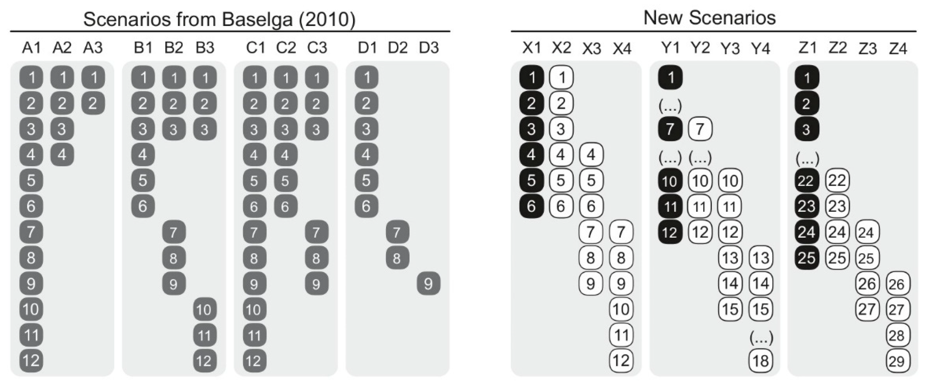
Table 1), we used two sets of scenarios (
Figure 1). First, we retrieved the four hypothetical scenarios used in Baselga [
14] (p. 135, examples A–D) that aim to account for (i) nestedness, (ii) spatial turnover, (iii) nestedness and spatial turnover, as well as (iv) differences in richness (referred to as Baselga’s Scenarios hereafter). Second, given that Baselga’s Scenarios seem simplistic, we generated a set of scenarios differing in species richness that contrast a reference hypothetical assemblage with assemblages sharing all species, sharing half of the species, and sharing no species as follows: 1:1 (i.e., 6 vs. 6 sp.), 1:0.5 (i.e., 12 vs. 6 sp., and 1:0.16 ratios (i.e., 25 vs. 4 sp.) (referred to as new scenarios hereafter;
Figure 1). We used this set of new scenarios in order to test if the role of species richness differences controlling for the number of shared species changed in relation to Baselga’s Scenarios. We are specifically considering highly contrasting assemblage arrangements that resemble those commonly found in conditions of the Anthropocene (e.g., grazing pastures, croplands, urban settings [
36]).
We generated pairwise calculations for Baselga’s Scenarios and the new scenarios using the functions ‘betadiver’ and ‘betapart’ [
34] of the package ‘vegan’ [
35] for R [
37]. Given that, to our knowledge, no function or R package calculates β
rich, β
rich.s, β
-3.s, we included the formulas of these measures in ‘betadiver’ as expressed in Baselga and Leprieur [
17] (see
Table 1 for details). In order to assess the similarities/dissimilarities of the results of the assessed measures, we performed a two-dimension non-metric multidimensional scaling (NMDS) analysis using Euclidean distances. For consistency, we re-expressed all results for these analyses to dissimilarity and present them in the
Supplementary Material. We followed an NMDS approach as it represents one of the most robust unconstrained ordination methods in ecology to graphically represent the similarities among the assessed measures in a two-dimensional plot, often summarizing more information in a lower number of axes and lacking limitations regarding sample size, scale, and normality [
38]. In order to validate our interpretation of the NMDS grouping, we ran an analysis to fit the interpreted groupings (a vector) to the ordination using the ‘envfit’ function for the package ‘vegan’ (beta calculations can also be run on BAT [
39]).
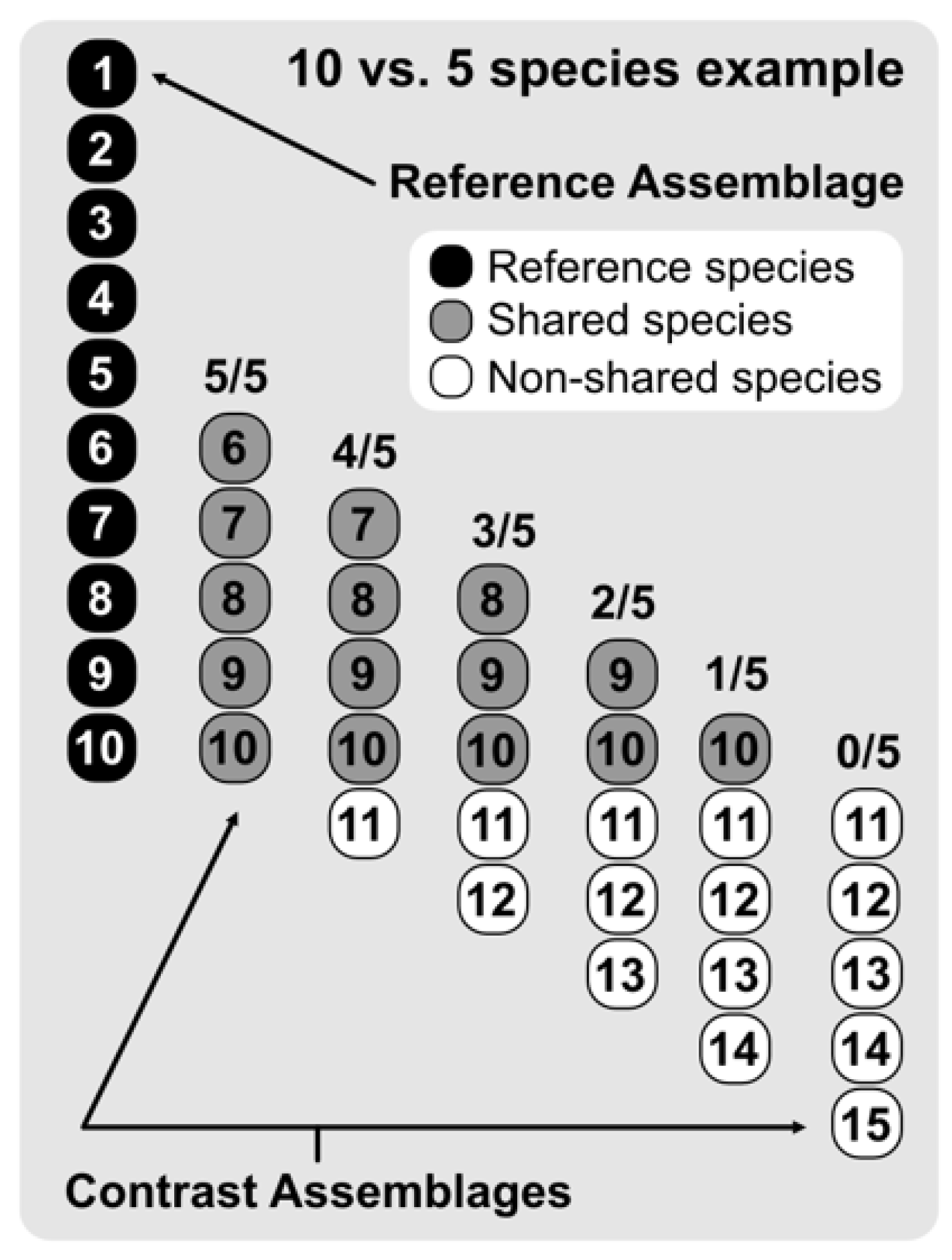
We then assessed the results of the 12 measures through gradual species composition overlap between paired assemblages, considering progressive differences in species richness (
Figure 2). This approach allowed us to record the results of the 12 focal indices in differing species richness and overlap scenarios. Briefly, we contrasted 10 hypothetical assemblages (Assemblage B
n) ranging from 1–10 species with a 10 species reference assemblage (Assemblage A). To evaluate differences in gradual species composition overlap, we performed pairwise calculations between Assemblage A and Assemblages B
1–10, retrieving the results for all possible combinations ranging from sharing all species to sharing none (see
Figure 2 for a graphical example of 10 vs. 5 species). This procedure would not only show how the studied indices behave when gradually changing from entirely nested to entirely turned over, but also assess the importance of differences in species richness between the gradually overlapped paired assemblages on β-diversity measures and results.
We further tested potential relationships between the total species richness of randomly generated paired assemblages and the results of the 12 assessed indices. For this, we generated 100 paired random assemblages ranging from 11 to 1000 species with three different richness ratios: 1:1, 1:0.5, and 1:0.1. We then retrieved the results of the 12 assessed indices for all randomly generated paired assemblages. Finally, in order to assess potential relationships between matrix size and the type of results and the studied indices, we calculated Spearman correlations for the results of all assessed indices and the total species richness of randomly generated paired assemblages (matrix size;
Figure S1) considering highly conservative Holm–Bonferroni sequential adjustments of
p-values [
40].
It is of the utmost importance to clarify that, given the goal of this study, which is to assess the type of results of the 12 measures calculated using the trending environment for statistical computing R [
37], we kept the original formulas (some of similarity, others of dissimilarity) and thus did not re-express formulas to homogenize results (as performed in some previous studies; e.g., Koleff et al. [
12]; Baselga and Leprieur, [
17];
Table 1) for our gradual species composition overlap (yet, we do include the homogenized results in
Figure S2). The latter ensures that the interpretation of the results is not misguided in relation to the original description of the measures. Nonetheless, we have included results with re-expressed formulas in the
Supplementary Material in order to allow comparisons with previous studies.
3. Results
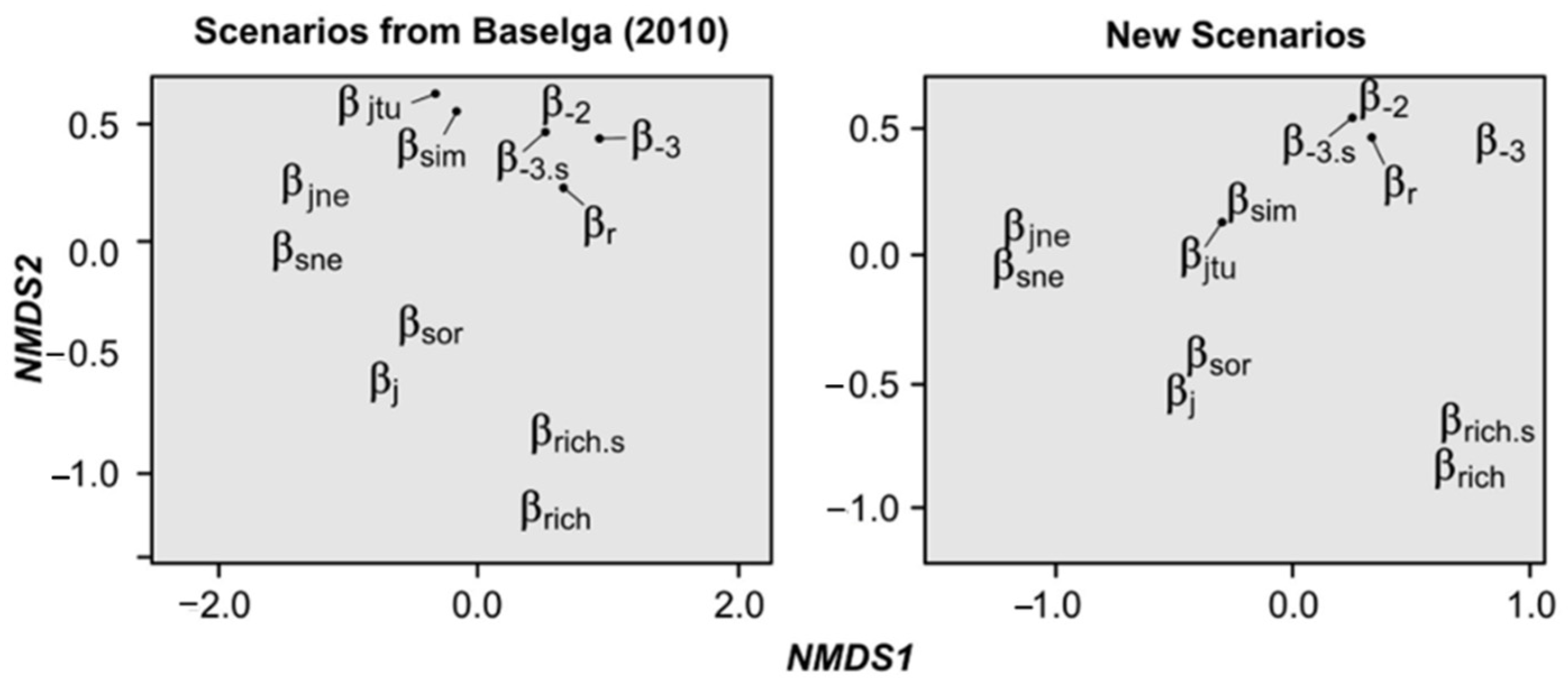
Through NMDS ordinations, we found that the retrieved similarity/dissimilarity values of all calculations were highly similar between both sets of hypothetical scenarios, showing that Baselga’s Scenarios are robust for index assessment (
Table S1,
Figure 3). Both NMDSs were highly fit (Baselga’s scenarios: stress = 0.03, linear fit r
2 = 0.99; new scenarios: stress = 0.01, linear fit r
2 = 0.99), indicating that they are reliable. Interestingly, results of both NMDSs show that there are some measures whose results are highly similar, grouping them together in the two-dimensional space (with the new scenarios increasing their similarity). Specifically, we detected five groups: (i) both classic measures (i.e., β
j, β
sor), (ii) both nestedness measures (i.e., β
sne, β
jne), (iii) both measures that take into account species richness difference (i.e., β
rich, β
rich.s), (iv) both turnover measures (i.e., β
sim, β
jtu), and (v) the four remaining dissimilarity and replacement measures (i.e., β
r, β
-2, β
-3, β
-3.s). These groups were significantly correlated with the ordination of index results (Baselga’s Scenarios: r
2 = 0.97,
p = 0.001, new scenarios r
2 = 0.97,
p < 0.001).
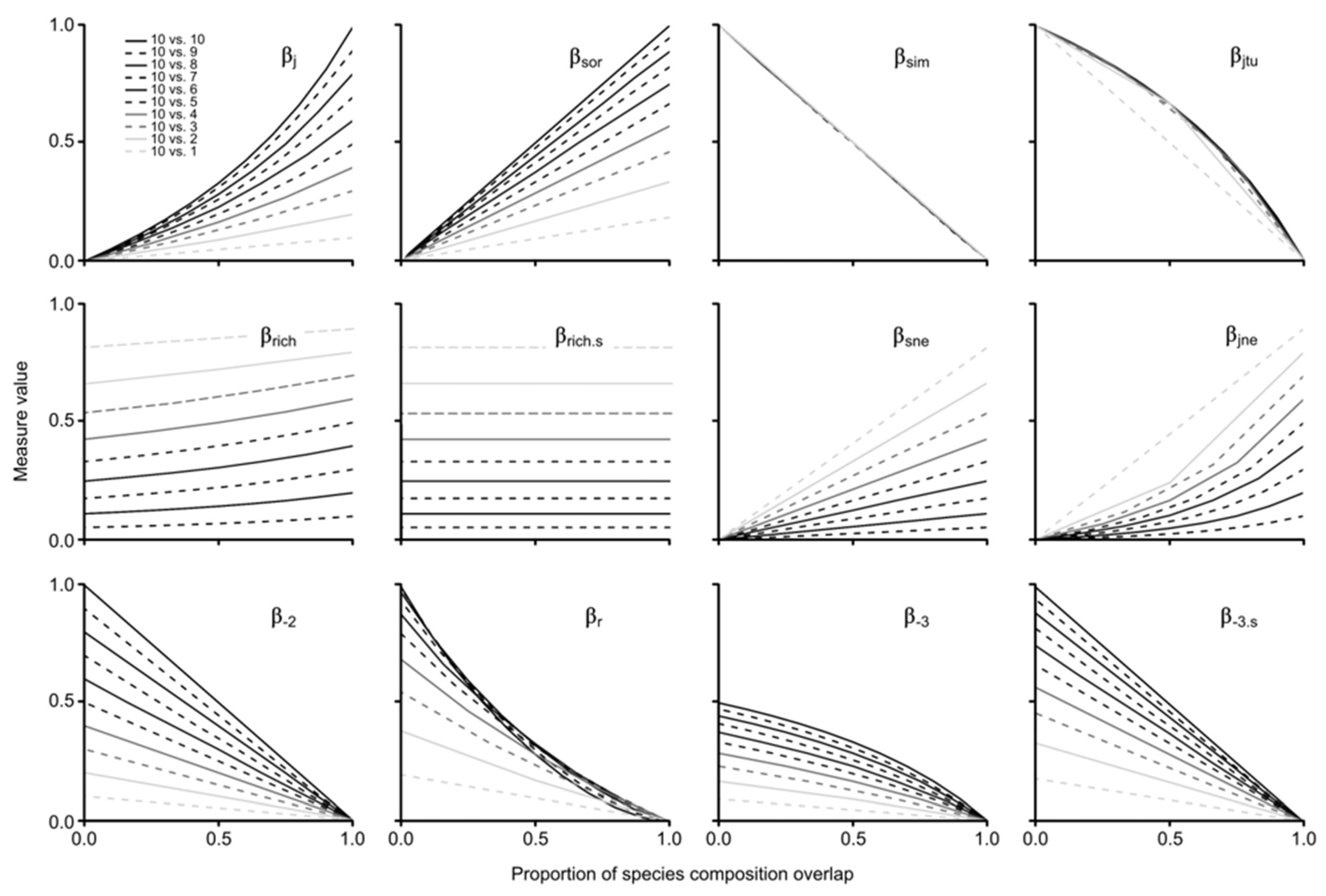
Regarding the gradual species composition overlap analysis between paired assemblages considering progressive differences in species richness, the results of the assessed measures were highly variable (
Figure 4). Here, we focus on the results of each measure by contrasting the groups shown by the NMDSs, some of which were expected, and some of which were not (i.e., group 5). For group 1, β
j and β
sor showed a positive increase in similarity with the proportion of assemblage overlap, which was heavily influenced by differences in species richness. It is noteworthy that β
sor increased linearly and β
j non-linearly (see
Figure S2 for results with re-expressed formulas to show dissimilarity patterns). For group 2, we found a positive increase in both measures (i.e., β
sne, β
jne) with the proportion of assemblage overlap, which was linear for β
sne and non-linear for β
jne (
Figure 4); both measures were also found to be highly influenced by species richness differences. Notably, none of the results of both measures reached 1, as expected due to the nature of the partition measure; maximum values were 0.82 for β
sne and 0.9 for β
jne, even in scenarios of 100% nestedness.
Both measures of group 3 (i.e., βrich, βrich.s) were very sensitive to changes in species richness; βrich.s behaved linearly and βrich tended to be non-linear. It is important to highlight that, on the one hand, βrich was mildly influenced by the proportion of overlap, with increasingly higher values between absent and total overlap (i.e., 10 vs. 9 sp. = 5%, 10 vs. 8 sp. = 9%, 10 vs. 7 sp. = 12%, 10 vs. 6 sp. = 15%, 10 vs. 5 and 4 sp. = 17%, 10 vs. 3 sp. = 16%, 10 vs. 2 sp. = 13%, 10 vs. 1 sp. = 8%). On the other hand, the results of βrich.s were not equidistant with differences in species richness, with larger intervals among higher values and smaller intervals among lower values (e.g., Δ βrich.s 1–2 sp. = 0.15; Δ βrich.s 9–10 sp. = 0.05).
Regarding turnover measures of group 4 (i.e., β
sim, β
jtu), both decreased with the proportion of assemblage overlap, with β
sim showing a linear pattern regardless of differences in species richness and β
jtu behaving non-linearly when the poorest assemblage has more than two species (given that the comparison with the assemblage of one species only generates two results that result in a linear response). For group 5 (i.e., β
r, β
-2, β
-3, β
-3.s), indices showed different patterns, but one general similarity: all retrieved unexpected values (>1) with no shared species when the species richness of the contrast assemblage was = 1–9. Moreover, β
-3 behaved non-linearly with maximum values = 0.5, and β
-r also showed non-linear results. β
-2 and β
-3.s decreased linearly with proportion of assemblage overlap; the former returned equidistant decreasing values with larger differences in species richness, and the latter returned lesser differences with lesser species richness differences (
Figure 4).
Finally, according to the assessment of index susceptibility to the matrix size (given by the total species richness of randomly generated paired assemblages), we found non-significant relationships with a 1:1 species richness ratio. We only recorded one moderate and significant relationship for β
rich.s with a 1:0.5 ratio, as well as two significant, moderate and weak, positive relationships for β
rich and β
rich.s, respectively (
Table S2;
Figure S1).
4. Discussion
More than half a century after Whittaker [
41] formally coined the definition of β-diversity, and over a century after Jaccard’s [
1] pioneering ‘coefficient of community’ approach, we still lack a consensus on the ways to quantify it in any of its expressions (see Moreno and Rodríguez [
3]), as well as in the criteria for their use and ecological interpretation. Our results show that all assessed measures were not susceptible to matrix size (except β
rich and β
rich.s in scenarios with differing species richness, as would be expected due to their mathematical nature). Moreover, we show several performance aspects of the 12 assessed β-diversity measures worth taking into account when choosing indices, as well as when using and interpreting them. Results for the NMDSs were highly similar between the sets of hypothetical scenarios, both of which showed how the 12 assessed indices group in five clusters (classic measures: β
j, β
sor; nestedness measures: β
sne, β
jne; species richness difference methods: β
rich, β
rich.s; turnover measures: β
sim, β
jtu; remaining dissimilarity/replacement measures: β
r, β
-2, β
-3, β
-3.s). These findings indicate that, although differences exist, classic, nestedness, species richness difference, and turnover metrics retrieve results in a similar fashion.
In this section, we first focus on the measures that, having a ‘dissimilarity’ nature, returned values differing from 1, often when species richness was not equal between samples and in non-overlap scenarios (i.e., no shared species). Second, we address the implications of the non-linear responses of some of the assessed β-diversity measures to the gradual species composition overlap of paired assemblages. Third, we examine the results of both nestedness measures (i.e., β
sne, β
jne), the implications of using them as independent ‘nestedness’ measures, and the importance of verifying that the formulas used to calculate them agree with that of all components of the partitioned β-diversity. Fourth, we discuss the results of both richness difference measures (i.e., β
rich, β
rich.s) used in the partitioning of β-diversity (sensu Carvalho et al. [
16]; Legendre [
28]). Finally, we describe the type of results of the remaining β-diversity measures (i.e., β
sor, β
sim). It is important to underline at this point, as stressed in previous sections, that we did not re-express formulas to homogenize our gradual species composition overlap results, and that all discussions are based on the results retrieved using the aforementioned R packages (and formulas for β
rich, β
rich.s, and β
-3.s, provided in Baselga and Leprieur [
17]). Additionally, this section is mainly focused on the implications of the type of results of the assessed measures on their ecological interpretation, rather than on their mathematic nature.
Surprisingly, four of the assessed measures (i.e., β
-2, β
-3, β
-3.s, β
r), which are all dissimilarity metrics, returned values differing from 1 when no species were shared (in most cases when species richness was not equal; only β
-3 returned values different from 1 in all cases). As such, extreme caution must accompany their usage—even to the point of avoidance—given that the information they provide could lead to misinterpretations. β
r and β
-2 are dissimilarity measures that aim to take into account the degree of overlap related to total species richness, with the latter focused on unequally rich assemblages [
42,
43]; thus, it was completely unexpected for us to find such results. In the case of β
-3 and β
-3.s, both are replacement (turnover) measures (see Baselga and Leprieur [
17]). Thus, based on our results, we suggest avoiding the use of these indices unless the identified drawbacks are carefully considered in their interpretation.
Regarding the non-linear behavior of several measures (i.e., β
j, β
jtu, β
jne, β
r, β
-3), occurring in contrasts of assemblages with >1 species (i.e., 10 vs. 2–10 species), there are some issues that need to be taken into account when interpreting them. We recognize that the non-linear results are not incorrect, as they reflect the mathematical nature of the indices; nonetheless, we conclude that some aspects of such non-linearity should be taken into account when interpreting the results output by these indices. When contrasting two hypothetical assemblages with the same species richness (i.e., 10) using β
j, for instance, our findings indicate that when the assemblages share half of their species (50% overlap), the result is 0.33. Although β
j is a dissimilarity index (when expressed as suggested by Baselga and Leprieur [
17]) it is, as intended and expressed in its formula, returning the proportion of shared species in relation to the total list of implied species in the comparison. Thus, when considering β
j, users ought to take into account that results represent the proportion of shared species of the entire set of species in both samples. This could have important implications for further analyses when indices behave non-linearly (e.g., when gradual species composition overlap between paired assemblages was tested), particularly when linearity is assumed (e.g., Holz et al. [
44]; Qian and Ricklefs [
45]; Lasram et al. [
46]; Zhang et al. [
47]).
In general, the results of both evaluated nestedness measures (i.e., β
sne, β
jne) were similar, with the exception that β
sne responded linearly to gradual species composition overlap and richness differences and β
jne behaved non-linearly (see potential implications above). One important point to stress regarding these indices is that they are not direct measurements of nestedness, but the component of nestedness of the measured dissimilarity. Thus, the use of such indices as independent measures of nestedness per se or as dissimilarity measures is incorrect [
19,
29]. In cases where the aim is to assess nestedness through β
sne and/or β
jne, it is advisable to calculate the proportion of nestedness of the related dissimilarity index. For instance, in a scenario where Assemblage A has 20 species and Assemblage B has 10 species, all of which are shared with Assemblage A, β
sor = 0.33, β
sne = 0.33, and β
sim = 0.00. In this case, a measurement of nestedness would be β
sne/β
sor = 1.00, showing that there is 100% nestedness of Assemblage B on Assemblage A. Although similar results can be found for some scenarios using the Jaccard family (β
j and its nestedness partition β
jne), given their non-linear response to overlap recorded in this study, results can vary. For instance, when considering a scenario where the number of unique species of the assemblages is not equal (e.g., a = 10, b = 10, c = 1; only differing by 1 unique species in Assemblage B in relation to the last example), results differ between the Jaccard and Sørensen families, and, although Assemblage B is still quite nested in Assemblage A (10 if its 11 species are shared), β
sne/β
sor = 0.74 and β
jne/β
j = 0.68. This can be interpreted as a warning for the use and/or interpretation of such ratios and on the information provided by β-diversity nestedness measures under a partition framework. Yet, as indicated previously, the goal of this study is not focused on the assessment of β-diversity partitioning, nor on contrasting their results to a standard.
As recommended for both assessed nestedness measures, those focused on reflecting species richness differences (i.e., β
rich, β
rich.s) should also be used as components of the partition of compositional dissimilarities [
15,
17]. Both measures were found to be highly sensitive to differences in species richness, as expected, with β
rich.s showing no response to gradual species composition overlap and β
rich slightly increasing with overlap. Regardless of the type of results we retrieved with these indices, given the existence of robust procedures to contrast species richness among samples [
48,
49], β
rich and β
rich.s are not recommended to be used as measurements of differences in species richness per se.
The remaining measures, β
sor and β
sim, both from the Sørensen family [
17], responded linearly to gradual species composition overlap, with the former being sensitive to differences in species richness and the latter showing no effect. On the one hand, β
sor measures the average shared species in relation to the richness between both assemblages. This measure is easily interpretable when assessing gradual species composition overlap due to the linearity of its results. On the other hand, β
sim measures the number of shared species in relation to the sample with the least unique species, resulting in a useful index when contrasting numerous sets of assemblages with differing species richness. Both indices, as independent units, seem to be easily interpretable given the type of results retrieved in scenarios of gradual species composition overlap between paired assemblages with progressive differences in species richness.


 ,
, 


