Robust Object Segmentation Using a Multi-Layer Laser Scanner

Abstract

The major problem in an advanced driver assistance system (ADAS) is the proper use of sensor measurements and recognition of the surrounding environment. To this end, there are several types of sensors to consider, one of which is the laser scanner. In this paper, we propose a method to segment the measurement of the surrounding environment as obtained by a multi-layer laser scanner. In the segmentation, a full set of measurements is decomposed into several segments, each representing a single object. Sometimes a ghost is detected due to the ground or fog, and the ghost has to be eliminated to ensure the stability of the system. The proposed method is implemented on a real vehicle, and its performance is tested in a real-world environment. The experiments show that the proposed method demonstrates good performance in many real-life situations.

1. Introduction

With the recent developments in vehicular technology, advanced driver assistance system (ADAS) concept has spread rapidly; however, many problems still remain to be addressed before the field of ADASs can be widely expanded. The biggest problem in ADAS is the use of sensor measurements and recognition of the surrounding environment. To this end, several types of sensors have been considered, including radar and a visual or infrared (IR) camera. Unfortunately, however, none of the sensors are sufficient for ADAS, and each has its own shortcomings.

For example, radar returns relatively accurate distances to obstacles, but its bearing measurements are not accurate. Radar cannot recognize object classes, and also suffers from frequent false detections [1–4]. A visual camera is another ADAS tool. This type of camera returns a relatively accurate bearing to the obstacle, but its distance measurement is not reliable. The camera is capable of object recognition, but it also exhibits a high false detection rate. Thus, most of the current systems combine several sensors to compensate for the drawbacks of each sensor and to obtain reliable information about the nearby environments [5–9].

Recently, the laser scanner has received attention within the ADAS community, and it is considered to be a strong candidate for the primary sensor in ADAS [1,10]. The strong points of the laser scanner are its ability to accurately determine both near and far distances as well as the bearing to an obstacle. In addition, the object detection of a laser scanner is reliable and robust, and it can recognize object classes to some extent through determination of the contour of the surrounding environment.

Thus, unlike a camera or radar, a laser scanner can be used as the sole sensor for ADAS without being combined with other sensors. Further, if the laser scanner is combined with other sensors, it can compensate for all the drawbacks, thereby improving the recognition accuracy.

Because the range and bearing measurements of the laser scanner are sufficiently accurate, in this paper, the laser scanner is considered as a single sensor for ADAS. In this paper, the laser scanners are divided into three types according to the number of layers; single-layer, multi-layer, and three-dimensional (3D) laser scanners. A single-layer laser scanner consists of only one layer, a multi-layer laser scanner is composed more than one but fewer than eight layers, and a 3D laser scanner is composed of eight or more layers. A single-layer laser scanner can obtain 2-dimensional (2D) information, a 3D laser scanner can get 3D information, and a multi-layer laser scanner can get limited 3D information. In general, the information from a laser scanner is proportional to the number of layers, but a 3D layer scanner is expensive and difficult to install on the vehicle. However, single-layer and multi-layer laser scanners can be implemented inside a vehicle's body [11]. Therefore, the 3D layer scanner is not yet suitable for ADAS, and the multi-layer laser scanner is currently more suitable for ADAS.

The remainder of this paper is organized as follows: in Section 2, an outline of the obstacle recognition system using a laser scanner is described. Related works are described in Section 3. The segmentation for a multi-layer laser scanner and the ghost elimination are explained in Section 4. The proposed system is installed on a vehicle and is applied to actual urban road navigation. The experimental results are presented in Section 5. The discussion about robustness is described in Section 6. Finally, some conclusions are drawn in Section 7.

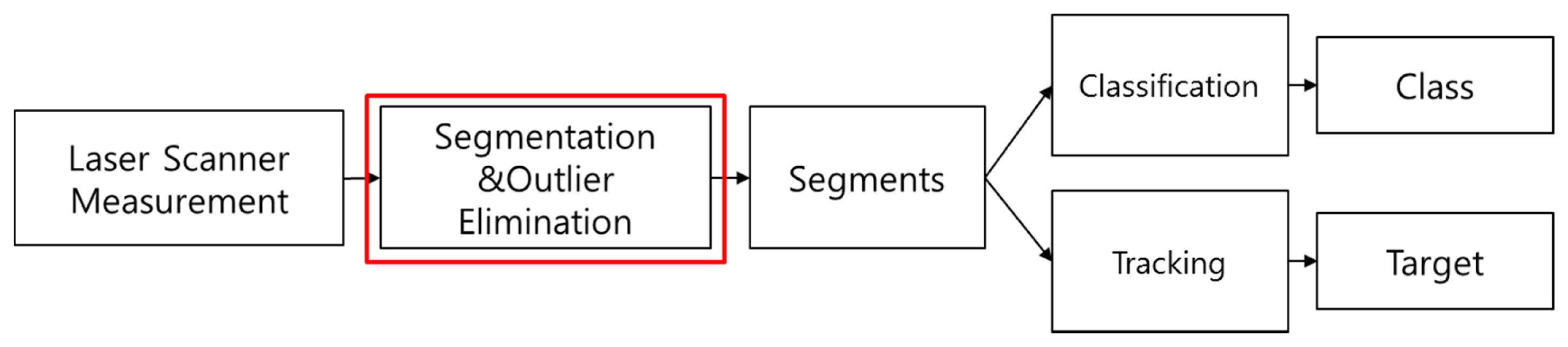
2. System Outline

The system aims to detect obstacles through the processes of segmentation, classification, and tracking. Figure 1 shows the outline of the system developed in this paper.

In the segmentation step, the proposed system receives a full scan (a set) of measurement points from a multi-layer laser scanner and decomposes the set into several segments, each of which corresponds to an object. In the segmentation step, the outliers are removed to avoid performance degradation. In the classification step, the segment features are computed and classified [12–14]. In the tracking step, the location and velocity of the segment are estimated over time. Segmentation is the essential step to execute classification or tracking [15–18]. In this paper, we focus on the methods for segmentation and outlier elimination.

3. Related Works

A laser scanner detects the closest obstacle for a bearing angle and returns the angle-wise distance to the obstacle. The output of the laser scanner can be modeled by the following set of pairs:

$$Z^t=\left\{p_1^t,p_2^t,p_3^t,\cdots ,p_N^t\right\}$$

(1)

$$p_i^t=\left(r_i^t,{\theta }_i^t\right)\mathit{\text{for}}i=1,\dots ,N$$

(2)

$${\theta }_i^t>{\theta }_{i-1}^t\mathit{\text{for}}i=2,\dots ,N$$

(3)

where N denotes the number of scanner measurement points as shown in Figure 2; the superscript t denotes the measurement time; and $r_i^t$ and ${\theta }_i^t$ denote the distance and bearing to the obstacles, respectively. Equation (3) refers to a property of the laser scanner, and it implies that the scanner scans the environment from left to right. As stated in Section 2, segmentation is the first step for the object detection by the laser scanner. A scan of the measurements, as given in Equations (1) and (2), is decomposed into several groups called segments, as shown in Figure 2.

In general, the segmentation methods can be classified into two kinds: the geometric shape method and the breakpoint detection (BD) method. The first method assumes the geometric shapes of the segments, such as a line or an edge, and decomposes the scanner measurements into the predetermined shapes [19,20]. The BD method decomposes the scanner measurements into segments based on the Euclidean distance between the consecutive points $p_i^t$ and $p_{i-1}^t$ [21] or using a Kalman filter [22]. Methods using BD based on the distances between consecutive points are the most popular and are widely used for laser segmentation [23–27].

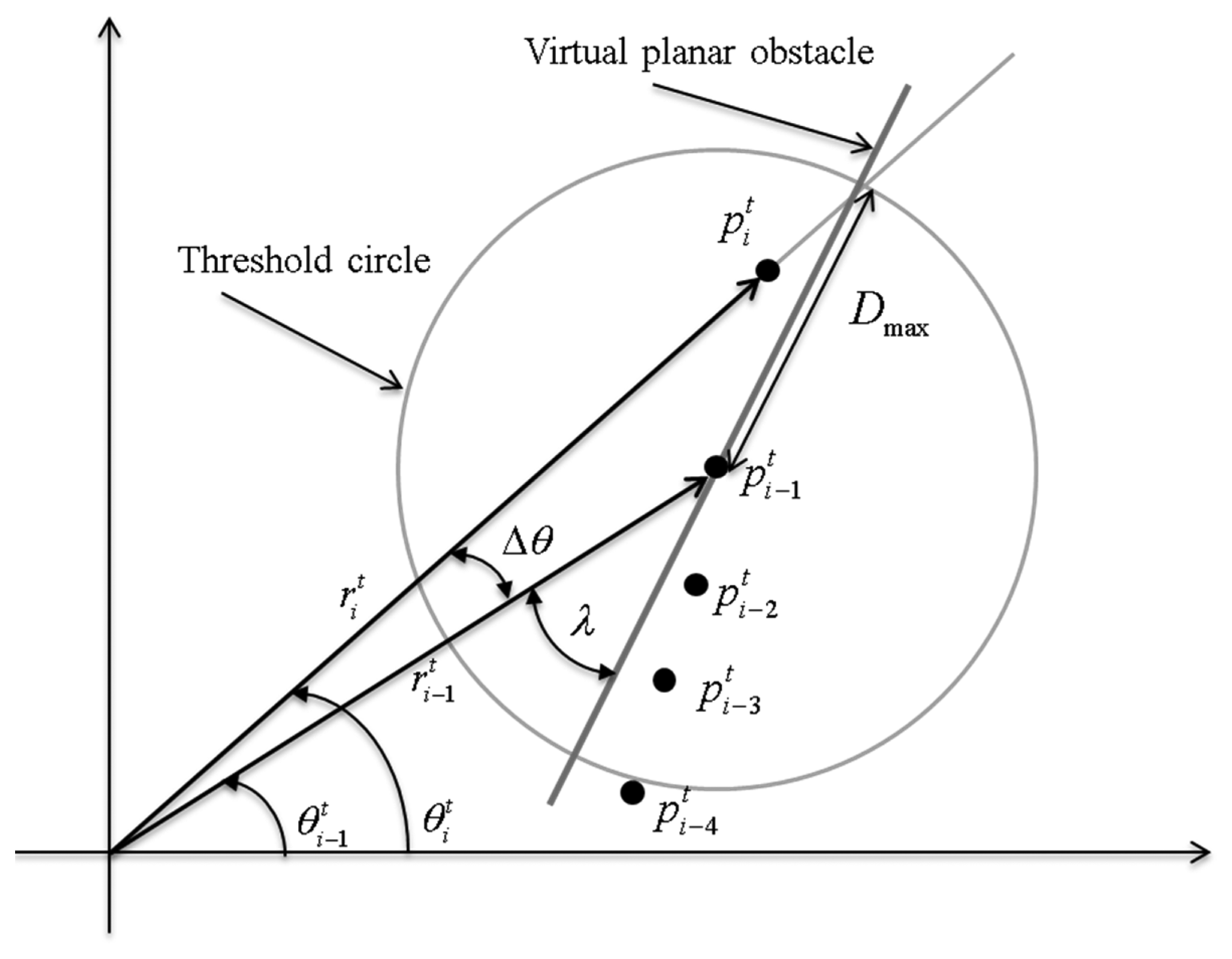
In the distance-based BD, if the distance between two consecutive points is greater than a threshold D_thd, two points are likely to belong to different objects and a breakpoint is selected between the two points as shown in Figure 2a.

In Figure 2, the laser scanner returns 12 data points ( $p_1^t-p_{12}^t$) and the segment S_n originates from the n th object (n = 1,2,3). The performance of the BD segmentation depends on the choice of a threshold D_thd, and several methods have been developed for the selection of D_thd. In [23], the threshold D_thd is determined by:

$$D_{\mathit{\text{thd}}}=C_0+C_{1}min\left\{r_i^t,r_{i-1}^t\right\}$$

(4)

where $C_1=\sqrt{2\left(1-cos\left({\theta }_i^t-{\theta }_{i-1}^t\right)\right)}$ and C₀ denotes the sensor noise. In [24], Lee et al., employed Equation (5) to select the break points in [17].

$$D_{\mathit{\text{thd}}}=\left|\frac{r_i^t-r_{i-1}^t}{r_i^t+r_{i-1}^t}\right|$$

(5)

Borges et al., recently proposed the adaptive breakpoint detector (ABD) in [25]. In the ABD, the threshold D_thd is determined by:

$$D_{\mathit{\text{thd}}}=r_{i-1}^t\cdot \frac{sin\left(\mathrm{\Delta }\theta \right)}{sin\left(\lambda -\mathrm{\Delta }\theta \right)}+3{\sigma }_r$$

(6)

which adaptively depends on $r_{i-1}^t$ and Δθ as shown in Figure 3. In Equation (6), $\mathrm{\Delta }\theta ={\theta }_i^t-{\theta }_{i-1}^t$, where λ is chosen on the basis of user experience, and σ_r is the sensor noise associated with r.

All of the previous segmentation methods, however, were based on a single-layer laser scanner, and to our knowledge, no research has been reported regarding the segmentation for a multi-layer laser scanner. This is one of the contributions of this paper.

4. Segmentation for Multi-Layer Laser Scanner

4.1. ABD Segmentation for Multi-Layer Laser Scanner

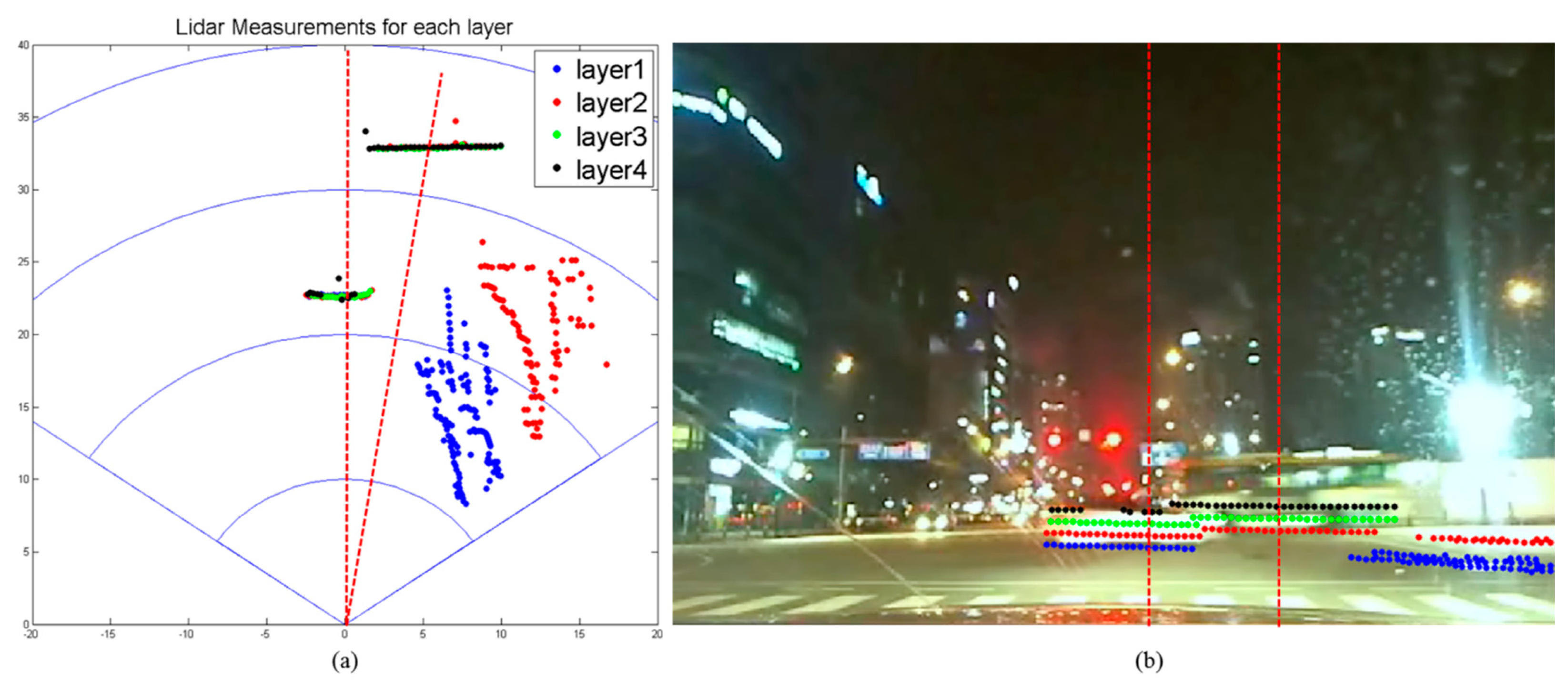
A multi-layer laser scanner has multiple layers and returns the measurement points as shown in Figure 4.

Figure 4a shows the laser scanner measurements depicted on the x-y plane, and Figure 4b shows the scanner measurements superimposed on the camera image after calibration [28]. In the figure, the information of the different layers is represented by different colors. In the multi-layer laser, each data point $p_i^t$ is not a pair but a triplet consisting of the distance $r_i^t$ and bearing ${\theta }_i^t$ to the obstacle and the layer information $l_i^t$. The output of the multi-layer laser scanner is modeled by:

$$\begin{array}{cc}{p}_i^t=\left(r_i^t,{\theta }_i^t,l_i^t\right)& \mathit{\text{for}}\end{array}i=1,\dots ,N$$

(7)

$$\begin{array}{cc}{\theta }_i^t\ge {\theta }_{i-1}^t& \mathit{\text{for}}i=2,\dots ,N\end{array}$$

(8)

$$\begin{array}{cc}{l}_i^t\ge l_{i-1}^t& \text{where}\end{array}{\theta }_i^t={\theta }_{i-1}^t$$

(9)

where a four layer laser scanner, the IBEO LUX2010 [29], is used, and:

$$l_i^t\in \left\{1,2,3,4\right\}$$

(10)

Equations (8) and (9) refer to the property that the scanner scans the laser from left to right and from bottom to top, respectively. The left points are measured before the right points and at the same ${\theta }_i^t$, and the lower layers are measured before the upper layers. The direct application of a standard ABD to multi-layer segmentation would lead to the loss of layer information and would lead to inefficient segmentation.

In order to develop a new segmentation method for the multi-layer scanner, two important properties of the multi-layer laser scanner should be considered:

(1)

Two points at the same bearing but on different layers can belong to different objects. An example is the situation given in Figure 4. In the figure, both a sedan and a bus lie in the same bearing, but the sedan is closer to the scanner than the bus. From the box bounded in red dotted lines in Figure 4b, the points in the lower three layers belong to the sedan, but the points in the top layer belong to the bus. Thus, it must be determined whether or not two data points, $p_i^t$ and $p_j^t$, with consecutive bearings and consecutive layers belong to the same object.

(2)

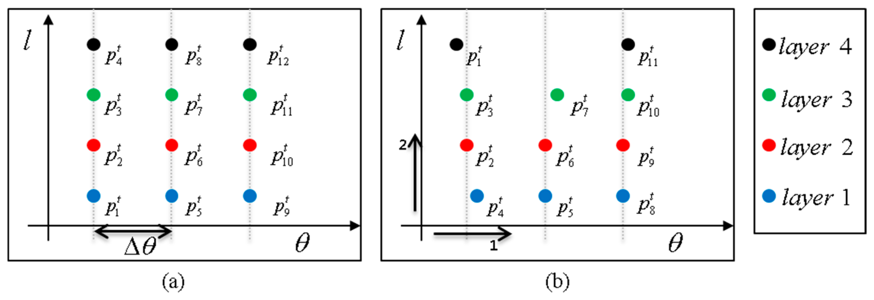
The measurement sets are not complete, and there are many vacancies in the θ - l plane. When the scanner input is plotted on the θ - l plane, the ideal output will look like a grid as in Figure 5a, but the actual output appears as in Figure 5b. Thus, the grid-type segmentation using a nested for-loop cannot be used.

A layer-wise independent segmentation process can be considered; however, in our experience, this method does not work well and requires multi-layer segmentation. In multi-layer laser segmentation, we will say that two points $p_i^t$ and $p_j^t$ are connected if they belong to the same object. Unlike single-layer scanner segmentation, we consider not only the connectivity between the points with consecutive bearings, but also the connectivity between the points with consecutive layers. The foremost requirement in multi-layer segmentation is that the algorithm should operate in a single scan with the running time O(N), and the algorithm must not trace back to the old previous points, making it O(N²) or higher, where N is the number of measurement points.

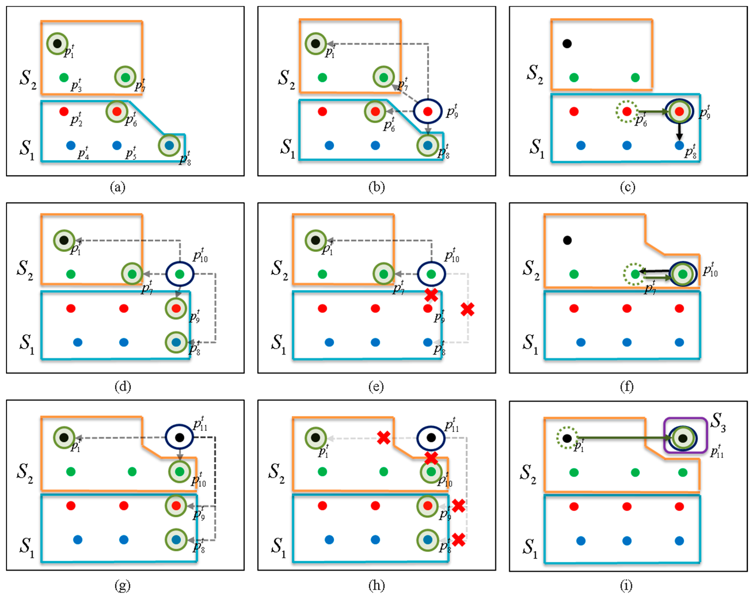
In this paper, an O(N) fast segmentation method is presented. When each data point $p_i^t$ is given, a candidate set _i composed of previous data points $p_j^t$ (j<i) is built, and the connectivity of the point $p_i^t$ is tested only with the elements in _i, thereby implementing an O(N) implementation. In our segmentation method, the candidate set _i consists of the newest data points in each layer. Therefore, the maximum size of the candidate set _i is four in this case. Figure 6 illustrates the ABD segmentation process.

In Figure 6, we assume that eight data points ( $p_1^t-p_8^t$) have already been received. $p_2^t$, $p_4^t$, $p_5^t$, $p_6^t$, and $p_8^t$ belong to the segment S₁, and $p_1^t$, $p_3^t$, and $p_7^t$ belong to S₂, as in Figure 6a. This situation occurs as in Figure 4, in which two vehicles are in the same direction but at the different distances. The candidate set ₉ is composed of $p_1^t$, $p_6^t$, $p_7^t$ and $p_8^t$. The four points in ₉ are the newest points in each layer at this time and the points in the set will be checked when a new point $p_9^t$ arrives. The points in ₉ are indicated by the green circles in Figure 6a.

In Figure 6b, $p_9^t$ is presented, and its connectivity with the elements in ₉ is determined in turn from the first to the fourth layers (in order of $p_8^t$, $p_6^t$, $p_7^t$, and $p_1^t$) with using an ABD. Here, we assume that the data point $p_9^t$ is assigned to the first segment as in Figure 6c. For example, if $\Vert p_9^t-p_8^t\Vert \le D_{\mathit{\text{thd}}}$, then $p_9^t$ is assigned to the segment of $p_8^t$, which is S₁, and further connectivity determinations with $p_6^t$, $p_7^t$, and $p_1^t$ are cancelled. Figure 6d-f show the segmentation of $p_{10}^t$. First, ₁₀ is computed by:

$$\begin{array}{ll}{\mathcal{M}}_{10}& ={\mathcal{M}}_9\cup \left\{p_9^t\right\}-\left\{p_6^t\right\}\\ & =\left\{p_1^t,p_7^t,p_8^t,p_9^t\right\}\end{array}$$

(11)

in Figure 6d, where ∪ and − denote set union and subtraction, respectively. As before, the connectivity of $p_{10}^t$ with $p_8^t$, $p_9^t$, $p_7^t$, and $p_1^t$ is tested in turn (in order of $p_8^t$, $p_9^t$, $p_7^t$, and $p_1^t$). If $\Vert p_{10}^t-p_8^t\Vert >D_{\mathit{\text{thd}}}$ and $\Vert p_{10}^t-p_9^t\Vert >D_{\mathit{\text{thd}}}$ but $\Vert p_{10}^t-p_7^t\Vert \le D_{\mathit{\text{thd}}}$ as in Figure 6e, then $p_{10}^t$ is assigned to the segment of $p_7^t$, which is S₂, and further connectivity determination with $p_1^t$ is cancelled, as in Figure 6f.

In a similar way, $p_{11}^t$ is segmented in Figure 6g–i. As before, ₁₁ is updated by:

$$\begin{array}{ll}{\mathcal{M}}_{11}& ={\mathcal{M}}_{10}\cup \left\{p_{10}^t\right\}-\left\{p_7^t\right\}\\ & =\left\{p_1^t,p_8^t,p_9^t,p_{10}^t\right\}\end{array}$$

(12)

as in Figure 6g. The connectivity of $p_{11}^t$ is tested with the elements $p_8^t$, $p_9^t$, $p_{10}^t$ and $p_1^t$ in ₁₁ in turn. If all of the distances between $p_{11}^t$ and the elements in ₁₁ are larger than D_thd by $\Vert p_{11}^t-p_j^t\Vert >D_{\mathit{\text{thd}}}$ (j = 1,8,9,10), as in Figure 6h, then a new segment S₃ is created, and $p_{11}^t$ is assigned to S₃ (Figure 6i).

Table 1. ABD segmentation for multi-layer laser scanner.

S = ABD _ Segmentation _ for _ multi _ laayer _ laser _ sacanner(Zt)

1 S1 ← Ø, 1 ← Ø, Nseg ← 0

2 for i = 1 to N do

3 Select$p_i^t=\left(r_i^t,{\theta }_i^t,l_i^t\right)$

4 for all$p_j^t$ ∈ i do ⫽ i is candidate set

5 Select$p_j^t=\left(r_j^t,{\theta }_j^t,l_j^t\right)$

6 Calculate Dthd using ( $p_j^t$, ) by ABDa

7 if$\Vert p_i^t-p_j^t\Vert \le D_{\mathit{\text{thd}}}$ then ⫽ check the connectivity

8 $p_i^t$ where ∈ Sn ⫽ is added to the segment Sn

9 break

10 endif

11 endfor

12 if$p_i^t$ then ⫽ if is not connected any other point in i

13 Nseg ← Nseg + 1

14 $p_i^t$ ⫽ belong to new segment, SNseg

15 endif

16 Update i+1 from ( i, $p_i^t$)

17 endfor

^aABD is the adaptive breakpoint detector.

shows the proposed segmentation algorithm for the multi-layer laser scanner. In the table, N_seg denotes the number of segments, and N and L denote the number of data points and the number of layers, respectively. S₁ and ₁ are initialized with empty sets, and the segmentation proceeds from $p_1^t$ to $p_N^t.$

In the i th iteration, the connectivity of $p_i^t$ with the elements in _i is tested from the bottom layer to the top layer. The connectivity exist when the distance between $p_i^t$ and $p_j^t$ is smaller than threshold, D_thd. $p_j^t$ is one of elements in _i and D_thd is calculated using an ABD. If the $p_j^t$ is the first matching connected point, the $p_i^t$ is assigned to S_n. S_n is the segment that contains the first matching point $p_j^t.$

If $p_i^t$ is not close enough to any elements in _i and $p_i^t$ is not connected to any segment, then it means that $p_i^t$ belongs to a new segment and we increase N_seg by one. At the end of each iteration, we update the candidate set _i+1 using _i and $p_i^t.$

4.2. Robust Segmentation through Ghost Elimination

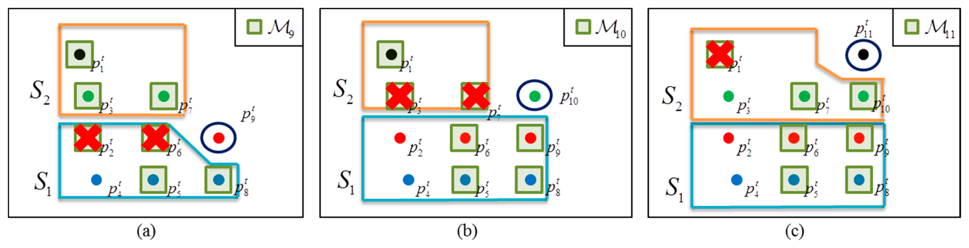
When the above ABD segmentation is applied to actual roads, ghost segments are sometimes detected. Here, a ghost segment refers to a segment that does not actually exist but that is detected by the laser scanner. Figures 7 and 8 show examples of ghost segments. These ghosts pose a serious risk to safe driving. Most ghost segments are caused by (1) laser reflections from the ground surface; or (2) lights from vehicles or fog. The false determination of a ghost segment seriously degrades the subsequent object classification performance.

Ghosts that are caused by reflections from the ground surface often occur when vehicles travel over bumpy roads or when they go up- or downhill. Ghost segments are detected on only one layer, usually the first layer, within a 40-m distance of the scanner, and experience rapid change, appearing and disappearing and changing shape. Ghosts that are caused by headlights or tail lights or by nearby fog are also detected on only a single layer within a 20-m distance of the scanner, do not have a uniform shape, and are detected intermittently.

The two kinds of ghosts both exist only on a single layer and are detected within a short distance. Thus, our robust segmentation method is developed by considering the first property and applying it within a limited 40-m distance around the vehicle. For distances greater than 40 m, the ABD segmentation method explained in Section 4.1 is used.

The robust segmentation method is similar to the ABD segmentation given in Section 4.1, with two main differences. The first difference is that when a point, $p_i^t$, is presented in robust segmentation, the point is not segmented with a point on the same layer in _i. The reason for this is that ghost points tend to gather only on a single layer. By not combining a new point with the points on the same layer, ghost points do not build a meaningful segment and thus are not considered. The second difference is that the candidate set _i consists of not one but two of the newest points in each other layer. To prevent an object from being divided due to a ghost, we determine the connectivity of up to two of the newest points in each other layer.

Thus, _i in robust segmentation can have up to eight (2×4) elements. Figure 9 illustrates the robust segmentation process. When a new point, $p_9^t$, is presented, as in Figure 9a, a candidate set, ${\mathcal{M}}_9=\left\{p_1^t,p_2^t,p_3^t,p_5^t,p_6^t,p_7^t,p_8^t\right\}$, is given. When testing the connectivity of $p_9^t$ with other points in ₉, we skip the test with $p_2^t$, and $p_6^t$ because they are on the same layer as $p_9^t$. Thus, the connectivities of $p_9^t$ are tested only with the five points { $p_1^t$, $p_3^t$, $p_5^t$, $p_7^t$, $p_8^t$ } in ₉, as shown in Figure 9a. Figures 9b and c demonstrate the computation of ₁₀ and ₁₁ and the robust segmentation process when $p_{10}^t$ and $p_{11}^t$ are given, respectively.

The problem with this approach is that if an obstacle is very shallow and is detected only on a single layer, it may not be detected. However, this is rarely the case due to the sufficiently small angular resolution of the multi-layer laser scanner. In the case of the IBEO LUX2010, the vertical and horizontal angular resolutions are 0.8° and 0.125°, respectively, allowing an obstacle 20 m or more from the vehicle and larger than 0.56 m to be detected on more than two layers. If the obstacle is larger than 0.26 m, it will return more than six points.

Table 2. Pseudo-Code of Robust Segmentation through Ghost Elimination.

S = Robust _ Segmentation(Zt)

1 S1 ← Ø, 1← Ø, Nseg← 0

2 for i = 1 to N do

3 Select$p_i^t=\left(r_i^t,{\theta }_i^t,l_i^t\right)$

4 if ( $p_i^t$) then ⫽ in a close area

5 for all$p_j^t$ ∈ i do ⫽ i is candidate set

6 Select$p_j^t=\left(r_j^t,{\theta }_j^t,l_j^t\right)$

7 if ( $p_j^t$) then ⫽ skip on same layer

8 Calculate Dthd using ( $p_j^t$, ) by ABDa

9 if$\Vert p_i^t-p_j^t\Vert \le D_{\mathit{\text{thd}}}$ then ⫽ check the connectivity

10 $p_i^t$ where ∈ Sn ⫽ is added to the segment Sn

11 break

12 endif

13 endif

14 endfor

15 else ⫽$p_i^t$ in a far area

16 for all$p_j^t$ ∈ i do ⫽ i is candidate set

17 Select$p_j^t=\left(r_j^t,{\theta }_j^t,l_j^t\right)$

18 Calculate Dthd using ( $p_j^t$, ) by ABDa

19 if$\Vert p_i^t-p_j^t\Vert \le D_{\mathit{\text{thd}}}$ then ⫽ check the connectivity

20 $p_i^t$ where ∈ Sn ∈ is added to the segment Sn

21 break

22 endif

23 endfor

24 endif

25 if$p_i^t$ then ⫽ if is not connected any other point in i

26 Nseg ← Nseg + 1

27 $p_i^t$ ⫽ belong to new segment, SNseg

28 endif

29 Update i+1 from ( i, $p_i^t$)

30 endfor

31 Eliminate small segments in S ⫽ S is the set of all segments Sn

^aABD is the adaptive breakpoint detector.

shows the pseudo-code of the robust segmentation. In lines 4-14, when a new point, $p_i^t$, is within 40 m of the scanner, the connectivity determination with the point on the same layer is skipped, as Figure 9. In lines 15–24, when a new point is far from the scanner, its connectivity with the point on the same layer is determined as the ABD segmentation. The processes of making new segment and updating candidate set, _i+l, is same as the processes of ABD segmentation. End of this algorithm, small segments are eliminated. The small segments mean the number of point is smaller than N_min, and N_min denotes the minimum number of points required for an object.

5. Experiment

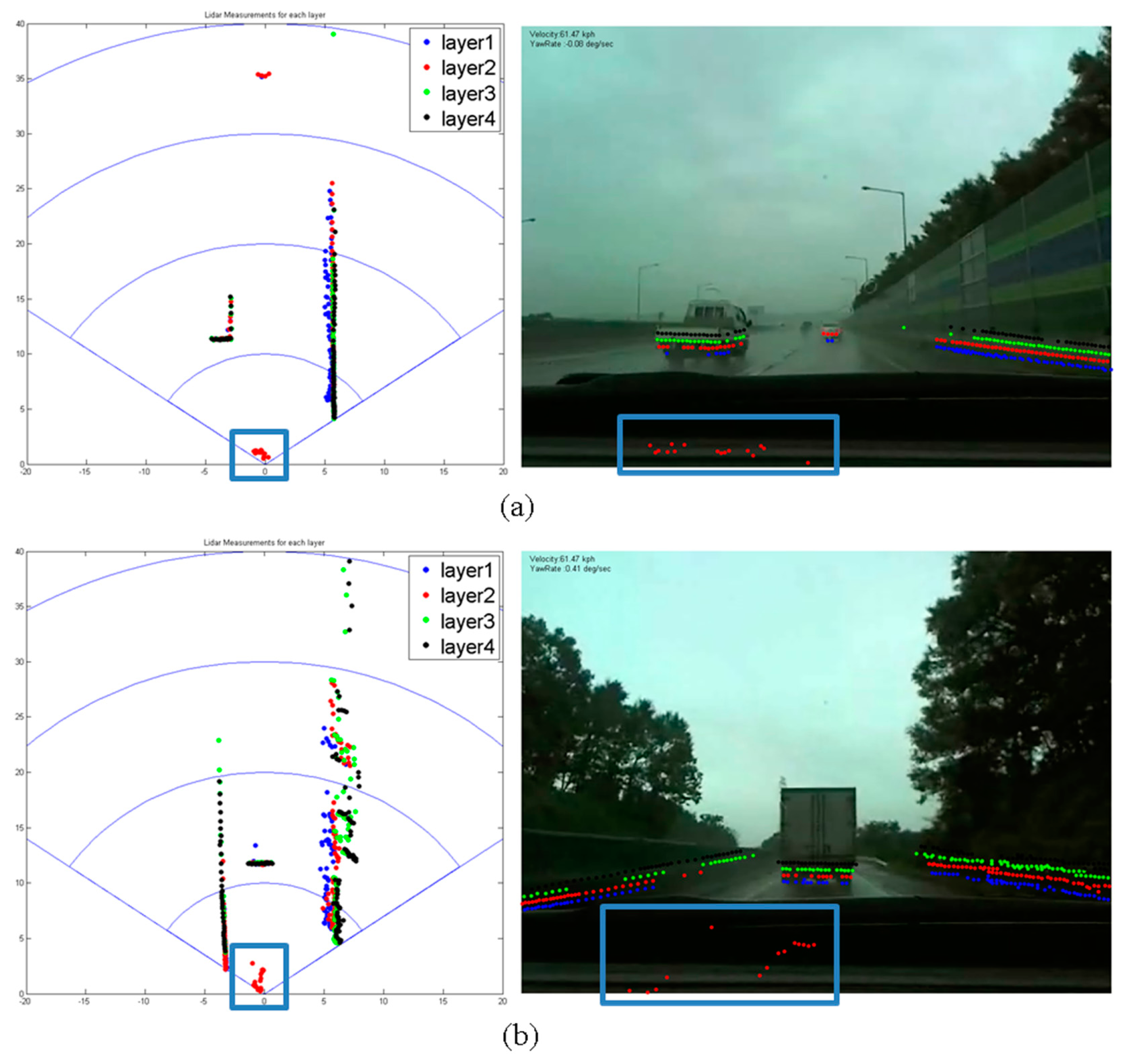
In this experiment, an IBEO LUX2010 multi-layer laser scanner and a camera are installed on a Kia K900 as shown in Figure 10. As previously stated, the LUX2010 has a total of four layers, and its horizontal and vertical resolutions are 0.125° and 0.8°, respectively. The camera is used to obtain the ground truth of the environment.

Figure 11 shows the segmentation results for six different scenarios. The first column shows the raw measurements from the IBEO scanner, and the second and third columns show the ABD and robust segmentation results, respectively. The fourth column contains the corresponding camera image with the scanner measurements superimposed.

Figure 11a and b show the results when the road is flat and ghosts are not detected. Only vehicles appear in Figure 11a, while both vehicles and pedestrians appear in Figure 11b. In the two scenarios, ghosts are not observed, and it can be seen that the ABD and robust segmentations produce the same results.

Figure 11c and d show the results when a ghost is detected that is created by the surface. In the figures, the dots in the red box are the ghost, detected by the bottom layer laser, which is indicated in blue. When the ABD segmentation method is applied (second column), the ghost forms an outlier segment and appears to be an obstacle. When the robust segmentation method is applied (third column), however, the ghost is successfully removed, leaving only the segments from the preceding vehicles.

Figure 11e and f show the results in rainy, foggy test conditions. As in Figure 11c and d, the dots in the red box are detected by the second-layer laser, and appear to result from fog. When the ABD segmentation method is applied (second column), the ghost survives and could activate the brake system, which can lead to an accident. When the robust segmentation method is applied (third column), however, the ghost is successfully removed. For quantitative analysis, we gather samples from four scenarios as in

Table 3. The number of ghosts, inliers, total measurement.

Circumstance	Ghost	Inlier	Total
Uphill road	4634	33,183	37,817
Plat road	1278	40,792	42,070
Rainy weather	2146	26,335	28,481
Foggy weather	1511	36,964	38,475

and apply the ABD and robust segmentation methods.

All the samples are clipped manually from the IBEO scan. In

Table 4. Results of ghost elimination for uphill road.

λ	ABD Segmentation			Robust Segmentation
	Ghost Elimination Ratio (%)	Inlier Survival Ratio (%)	Computation Time (ms)	Ghost Elimination Ratio (%)	Inlier Survival Ratio (%)	Computation Time (ms)
10	19.033	99.702	42.057	98.425	98.333	47.676
11	18.494	99.735	44.409	98.144	98.379	51.036
12	18.062	99.756	45.243	97.820	98.457	51.829
13	17.846	99.765	45.832	97.518	98.484	52.594
14	17.717	99.765	44.417	97.195	98.505	50.557
15	17.479	99.792	43.991	97.065	98.550	50.455

,

Table 5. Results of ghost elimination for flat road.

λ	ABD Segmentation			Robust Segmentation
	Ghost Elimination Ratio (%)	Inlier Survival Ratio (%)	Computation Time (ms)	Ghost Elimination Ratio (%)	Inlier Survival Ratio (%)	Computation Time (ms)
10	42.097	99.980	30.193	98.513	99.909	31.147
11	41.549	99.983	29.701	98.279	99.909	30.669
12	40.141	99.983	29.386	98.122	99.909	30.413
13	38.654	99.983	29.173	97.887	99.909	30.252
14	38.419	99.983	29.117	97.731	99.909	30.111
15	37.637	99.983	29.787	97.574	99.909	31.369

,

Table 6. Results of ghost elimination in rainy weather.

λ	ABD Segmentation			Robust Segmentation
	Ghost Elimination Ratio (%)	Inlier Survival Ratio (%)	Computation Time (ms)	Ghost Elimination Ratio (%)	Inlier Survival Ratio (%)	Computation Time (ms)
10	34.669	99.992	11.105	94.548	99.951	11.445
11	34.669	99.992	11.157	94.548	99.958	11.425
12	34.669	99.992	12.133	94.548	99.962	12.496
13	34.669	99.992	12.270	94.548	99.962	12.554
14	34.669	99.992	12.592	94.548	99.962	12.883
15	34.669	99.992	12.885	94.548	99.966	13.208

, and

Table 7. Results of ghost elimination in foggy weather.

λ	ABD Segmentation			Robust Segmentation
	Ghost Elimination Ratio (%)	Inlier Survival Ratio (%)	Computation Time (ms)	Ghost Elimination Ratio (%)	Inlier Survival Ratio (%)	Computation Time (ms)
10	63.269	99.946	21.019	97.088	99.221	23.411
11	63.203	99.946	20.161	97.022	99.261	22.484
12	63.137	99.951	20.711	96.956	99.294	23.019
13	63.071	99.954	20.983	96.889	99.294	23.375
14	63.071	99.957	21.439	96.889	99.321	23.961
15	62.674	99.959	22.869	96.823	99.359	25.473

, the results of the ghost elimination are described. The value of λ in Equation (6) is changed from 10° to 15°. The experiments are conducted in uphill road, flat road, rainy weather, and foggy weather conditions and their results are shown in Tables 4, 5, 6, and 7, respectively.

In the tables, the ABD and robust segmentation methods are compared in terms of (1) ghost elimination ratio; (2) inlier survival ratio and (3) computation time. Here, the ghost elimination ratio and the inlier survival ratio are defined as:

$$\mathit{\text{Ghost elimination ratio}}=\frac{\mathit{\text{The number of eliminated ghosts}}}{\mathit{\text{The number of ghosts}}}\times 100$$

(13)

$$\mathit{\text{Inlier survival ratio}}=\frac{\mathit{\text{The number of survived inliers}}}{\mathit{\text{The number of inliers}}}\times 100$$

(14)

From the tables, the proposed robust method outperforms the ABD in all cases with the similar computation time.

6. Discussion

Obviously, the goal is to remove as many ghosts as possible while maintaining as many inliers as possible and, thus to keep both ratios high. It can be seen from Tables 4, 5, 6, and 7 that the results of robust segmentation are better than those of ABD segmentation in every condition. In particular, the proposed robust method demonstrates more than 95% of the ghost elimination ratio in a robust manner regardless of the weather or the road. The ABD, however, demonstrates 17% to 65% of the ghost elimination ratio depending on the weather or the road. When it rains or the car goes uphill and, thus, ghosts frequently occur, ABD fails in eliminating the ghosts but the robust method removes most of the ghosts well. Interestingly, the ABD also performs well in the foggy weather and the reason is that the ghosts are detected intermittently in the foggy weather and they tend not to form a segment. Further, the ghost elimination ratio is not much affected by the value of λ. The reason might be that the ghosts are very close to the sensors and they are far enough from the other obstacles.

The inlier survival ratio is also an important factor because if the inlier is accidently removed by the algorithm, it will lead to a serious accident. The result of the inlier survival ratio is also shown in Tables 3, 4, 5, and 6. It can be seen that both of the segmentation methods have sufficiently high inlier survival ratios and the both algorithms do not accidently remove the important measurement points.

The ABD and robust segmentation methods are also compared in terms of computation time. The computation time in Tables 4, 5, 6, and 7 is obtained by computing the average over 100 frames. It can be seen that the robust method takes slightly longer time than the ABD but the extra time is not much. The reason is that the ghost tends to form a number of small segment and the elimination of them takes some time.

7. Conclusions

In this paper, a new object segmentation method for a multi-layer laser scanner has been proposed. For robust segmentation, efficient connectivity algorithms were developed and implemented with O(N) complexity. The proposed method was installed on an actual vehicle, and its performance was tested using real urban scenarios. It was demonstrated that the proposed system works well, even under complex urban road conditions.

References

- Keat, C.T.M.; Pradalier, C.; Laugier, C. Vehicle detection and car park mapping using laser scanner. Proceedings of the 2005 IEEE/RSJ International Conference on Intelligent Robots and Systems, 2005 (IROS 2005), Alberta, Canada, 2–6 August 2005; pp. 2054–2060.
- Mendes, A.; Bento, L.C.; Nunes, U. Multi-target detection and tracking with laserscanner. Proceedings of the 2004 IEEE Intelligent Vehicles Symposium, Parma, Italy, 14–17 June 2004; pp. 796–801.
- Fuerstenberg, K.Ch.; Dietmayer, K. Object tracking and classification for multiple active safety and comfort applications using a multilayer laser scanner. Proceedings of the 2004 IEEE Intelligent Vehicles Symposium, Parma, Italy, 14–17 June 2004; pp. 802–807.
- Gate, G.; Nashashibi, F. Fast algorithm for pedestrian and group of pedestrians detection using a laser scanner. Proceedings of the 2009 IEEE Intelligent Vehicles Symposium, Xi'an, China, 3–5 June 2009; pp. 1322–1327.
- Wu, S.; Decker, S.; Chang, P.; Camus, T.; Eledath, J. Collision sensing by stereo vision and radar sensor fusion. Trans. IEEE Intell. Transp. Syst. 2009, 4, 606–614. [Google Scholar]
- Oliveira, L.; Nunes, U.; Peixoto, P.; Silva, M.; Moita, F. Semantic fusion of laser and vision in pedestrian detection. Parttern Recognit. 2010, 43, 3648–3659. [Google Scholar]
- Premebida, C.; Ludwig, O.; Nunes, U. LIDAR and vision-based pedestrian detection system. J. Field Robot. 2009, 26, 696–711. [Google Scholar]
- Musleh, B.; Garcia, F.; Otamendi, J.; Armingol, J.M.; Escalera, A. Identifying and tracking pedestrians based on sensor fusion and motion stability predictions. Sensors 2010, 10, 8028–8053. [Google Scholar]
- Li, Q.; Chen, L.; Li, M.; Shaw, S.L.; Nuchter, A. A sensor-fusion drivable-region and lane-detection system for autonomous vehicle navigation in challenging road scenarios. IEEE Veh. Technol. Soc. 2014, 63, 540–555. [Google Scholar]
- Gidel, S.; Checchin, P.; Blane, C.; Chateau, T.; Trassoudain, L. Pedestrian detection and tracking in an urban environment using a multilayer laser scanner. Trans. IEEE Intell. Transp. Syst. 2010, 11, 579–588. [Google Scholar]
- Grisleri, P.; Fedriga, I. The braive autonomous ground vehicle platform. IFAC Symp. Intell. Auton. Veh. 2010, 7, 3648–3659. [Google Scholar]
- Lin, Y.; Puttonen, E.; Hyyppä, J. Investigation of Tree Spectral Reflectance Characteristics Using a Mobile Terrestrial Line Spectrometer and Laser Scanner. Sensors 2013, 13, 9305–9320. [Google Scholar]
- Premebida, C.; Ludwig, O.; Nunes, U. Exploiting LIDAR-based features on pedestrian detection in urban scenarios. Proceedings of the 12th International IEEE Conference on Intelligent Transportation Systems, St. Louis, MO, USA, 4–7 October 2009; pp. 1–6.
- Wender, S.; Fuerstenberg, K.Ch.; Dietmayer, K. Object tracking and classification for intersection scenarios using a multilayer laserscanner. Proceedings of the 11th World Congress on Intelligent Transportation Systems, Nagoya, Japan, 22 October 2004.
- García, F.; Jiménez, F.; Anaya, J.J.; Armingol, J.M.; Naranjo, J.E.; de la Escalera, A. The braive autonomous ground vehicle platform. Distributed pedestrian detection alerts based on data fusion with accurate localization. Sensors 2013, 13, 11687–11708. [Google Scholar]
- Jiménez, F.; Naranjo, J.E.; Gómez, Ó. Autonomous manoeuvring systems for collision avoidance on single carriageway roads. Sensors 2012, 12, 16498–16521. [Google Scholar]
- Ozaki, M.; Kakimuma, K.; Hashimoto, M.; Takahashi, K. Laser-based pedestrian tracking in outdoor environments by multiple mobile robots. Sensors 2012, 12, 14489–14507. [Google Scholar]
- Teixidó, M.; Pallejà, T.; Tresanchez, M.; Nogués, M.; Palacín, J. Measuring oscillating walking paths with a LIDAR. Sensors 2011, 11, 5071–5086. [Google Scholar]
- Mavaei, S.M.; Imanzadeh, R.H. Line Segmentation and SLAM for rescue robots in unknown environments. World Appl. Sci. J. 2012, 17, 1627–1635. [Google Scholar]
- Yang, S.W.; Wang, C.C.; Chang, C.H. Ransac matching: Simultaneous registration and segmentation. Proceedings of the 2010 IEEE International Conference on Robotics & Automation (ICRA), Anchorage, AK, USA, 3–7 May 2010; pp. 1905–1912.
- Skrzypczynski, P. Building geometrical map of environment using IR range finder data. Intell. Auton. Syst. 1995, 4, 408–412. [Google Scholar]
- Premebida, C.; Nunes, U. Segmentation and Geometric Primitives Extraction from 2D Laser Range Data for Mobile Robot Applications; Technical Report N° ISRLM2005/02; Institute of Systems and Robotics: Coimbra, Portugal, 2005. [Google Scholar]
- Dietmayer, K.; Sparbert, J.; Streller, D. Model based object classification and object tracking in traffic scenes from range images. Proceedings of the IV IEEE Intelligent Vehicles Sysposium, Tokyo, Japan, 13–17 May 2001.
- Lee, K.J. Reactive Navigation for an Outdoor Autonomous Vehicle. Master's Thesis, University of Sydney, Sydney, Australia, 2001. [Google Scholar]
- Borges, G.A.; Aldon, M. Line extraction in 2D range images for mobile robotics. Robot. Syst. 2004, 40, 267–297. [Google Scholar]
- An, S.Y.; Kang, J.G.; Lee, L.K.; Oh, S.Y. Line segment-based indoor mapping with salient line feature extraction. Adv. Robot. 2012, 26, 437–460. [Google Scholar]
- Jimenez, F.; Naranjo, J.E. Improving the obstacle detection and identification algorithms of a laserscanner-based collision avoidance. Transp. Res. Part C 2011, 19, 658–672. [Google Scholar]
- Zhang, Z. Flexible camera calibration by viewing a plane from unknown orientations. Proceedings of the Seventh IEEE International Conference on Computer Vision, Kerkyra, Greece, 20–27 September 1999; Volume 1, pp. 666–673.
- Homepage of IBEO Automotive Systems GmbH; Hamburg, Germany. Technical facts IBEO LUX 2010. Available online: http://www.ibeo-as.com/ (accessed on 28 October 2014).