
VisitSense: Sensing Place Visit Patterns from Ambient Radio on Smartphones for Targeted Mobile Ads in Shopping Malls

Abstract
:1. Introduction
2. Related Work
2.1. Indoor Localization
2.2. Place Detection and Recognition
2.3. Location Prediction
3. System Overview
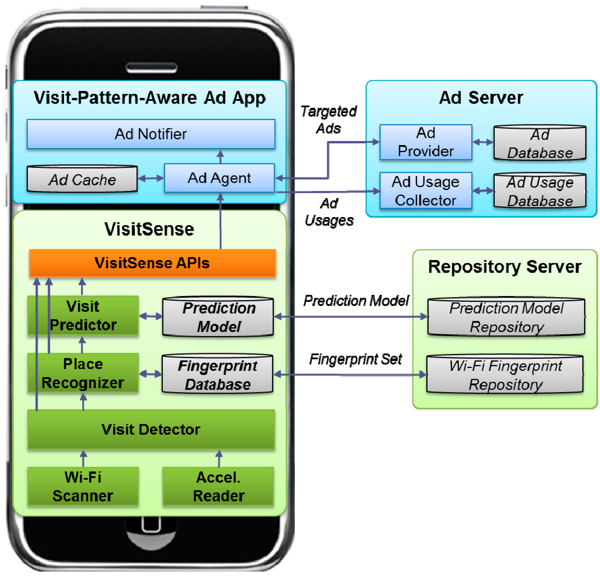
3.1. System Architecture


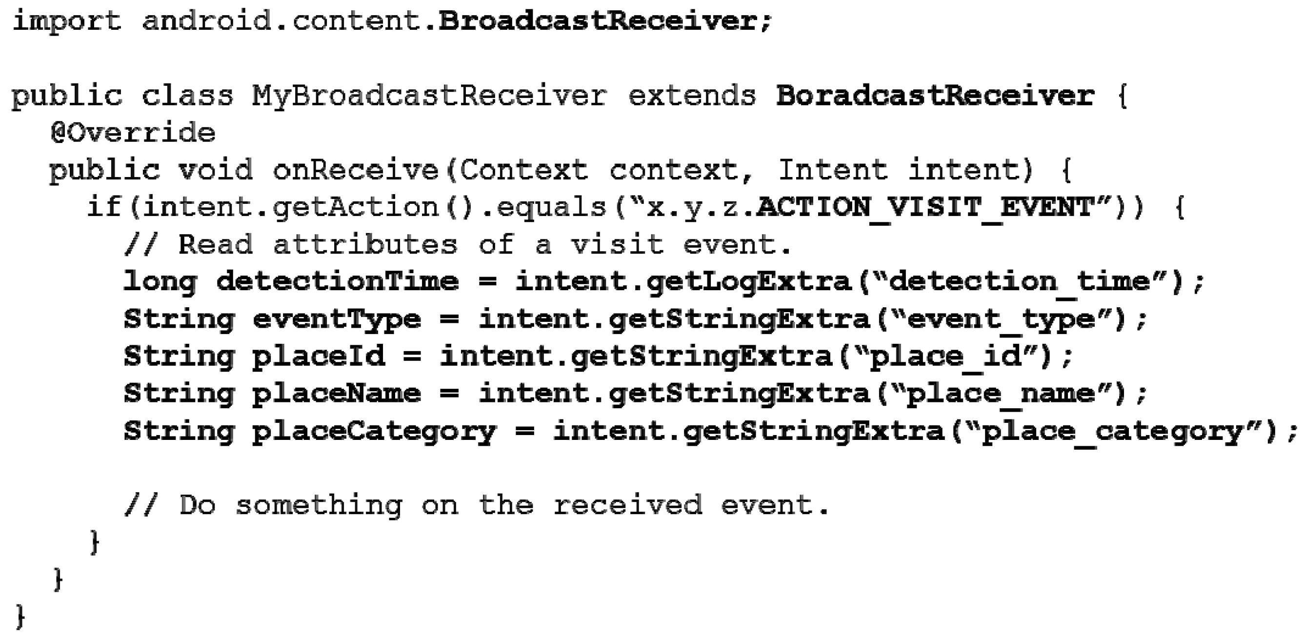
3.2. Application Programming Interface

3.3. Visit-Pattern-Aware Mobile Advertising
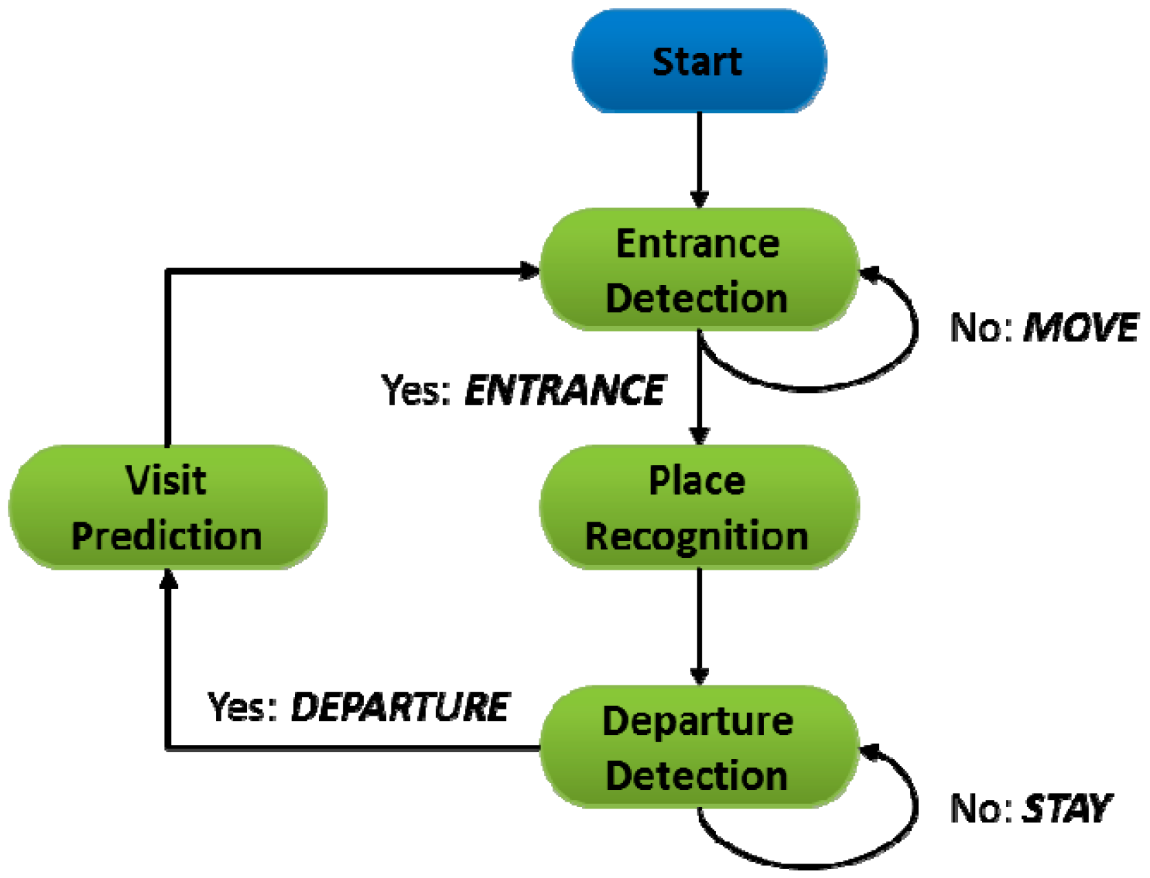
4. Main Operations
4.1. Visit Detection
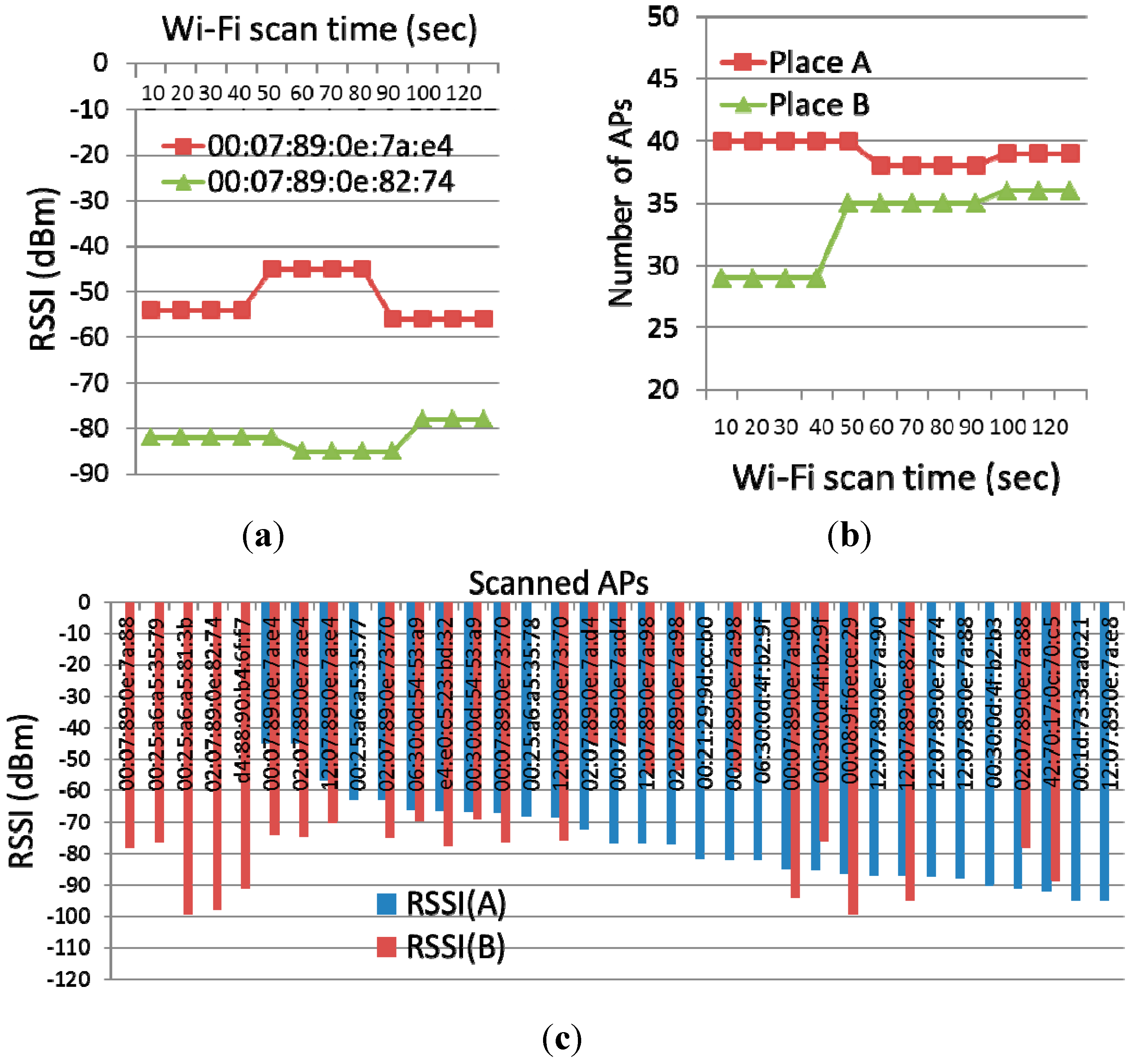
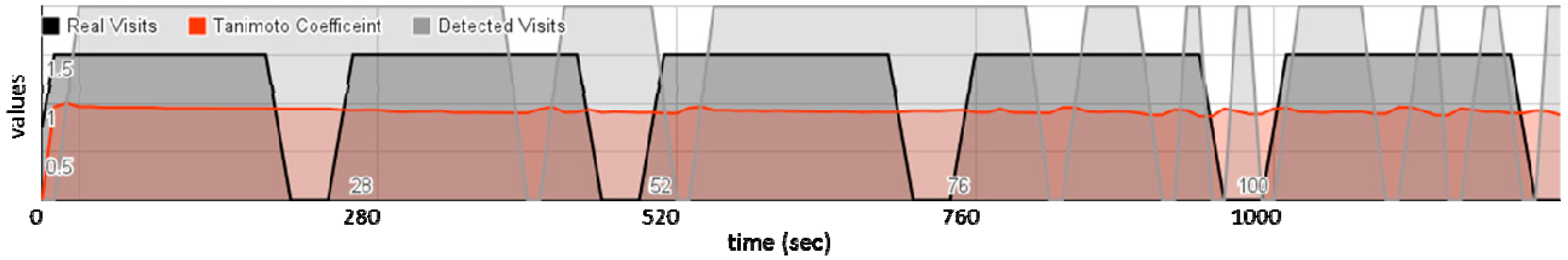
4.1.1. Challenge: Noisy Radio Ambience


| Algorithm | Formula |
|---|---|
| Jaccard coefficient | |
| Tanimoto coefficient | |
| Euclidean distance | |
| Pearson correlation coefficient |
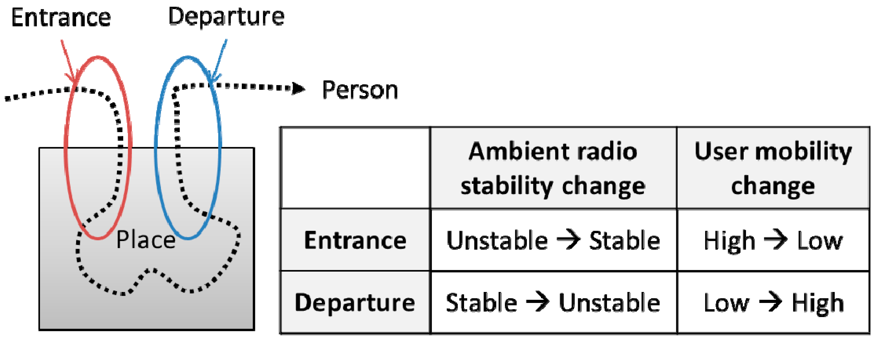
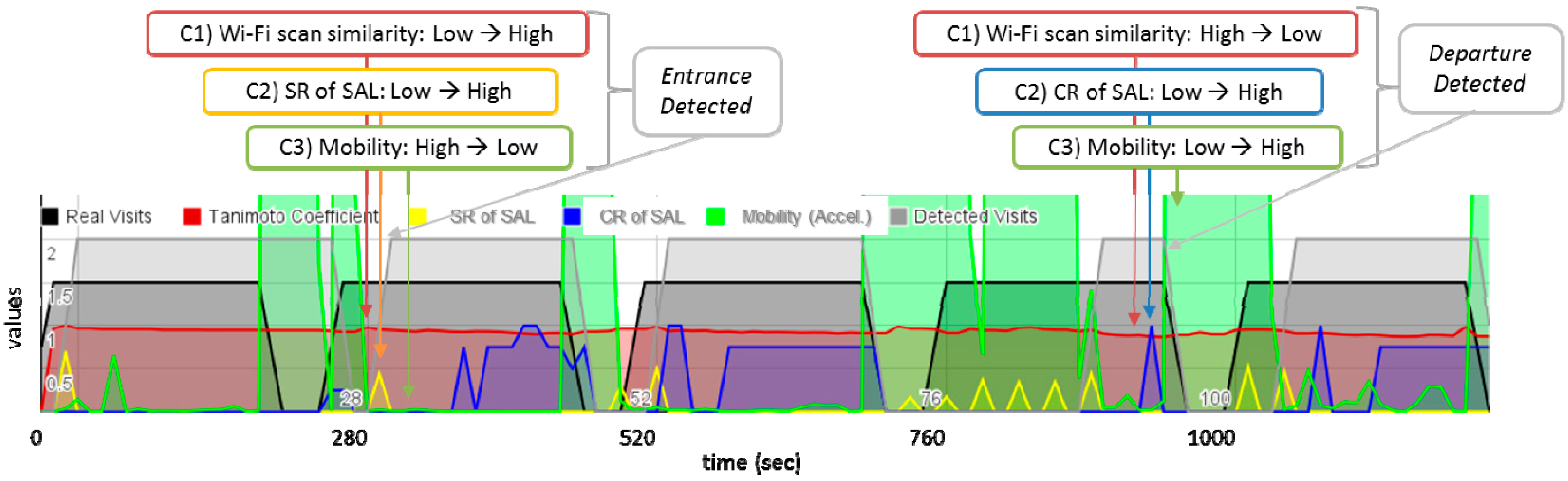
4.1.2. Change-Based Visit Detection


4.2. Place Recognition
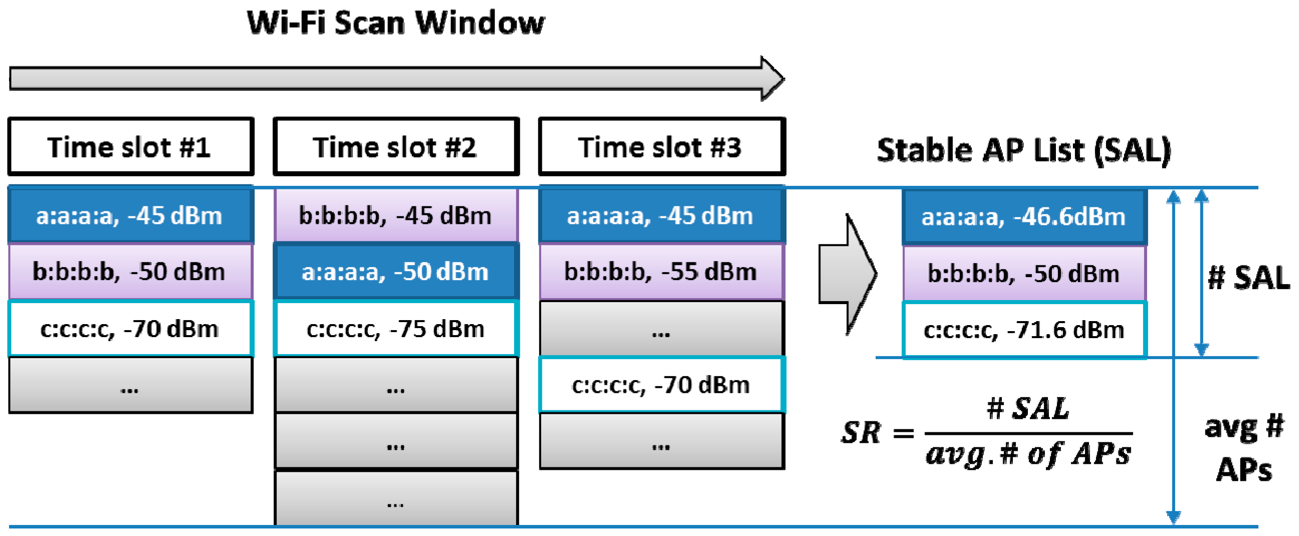
Noise-Filtered Wi-Fi Fingerprinting
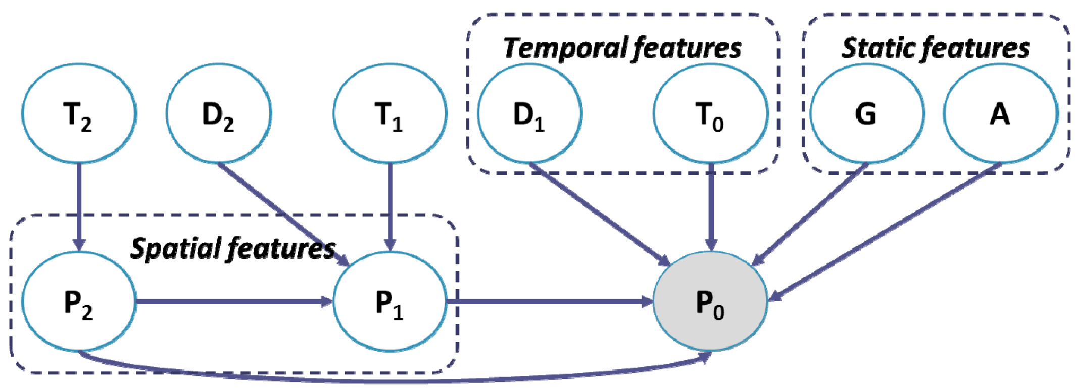
4.3. Visit Prediction
Causality-Based Visit Prediction Model

5. Evaluation
| Operation | Parameter | Values (* = default) |
|---|---|---|
| Wi-Fi Scan Window | Wi-Fi scan period | 10 *, 30 (s) |
| Wi-Fi scan window size | 3 * | |
| Wi-Fi Ambience Change Detection | Tanimoto similarity threshold | 0.9 * |
| Cutoff RSSI threshold | −60, −90 *, −120 (dBm) | |
| SR of SAL | 0.4 * | |
| Top-k AP RSSI change | 25 dBm * | |
| Mobility Change Detection | Accel. sampling frequency | 5 Hz * |
| Accel. window size | 300 (1 minute) * | |
| Mobility threshold | 3 * | |
| Place Recognition | Similarity algorithm | Tanimoto coefficient *, Jarccard coefficient, Euclidean distance, Pearson correlation coefficient |
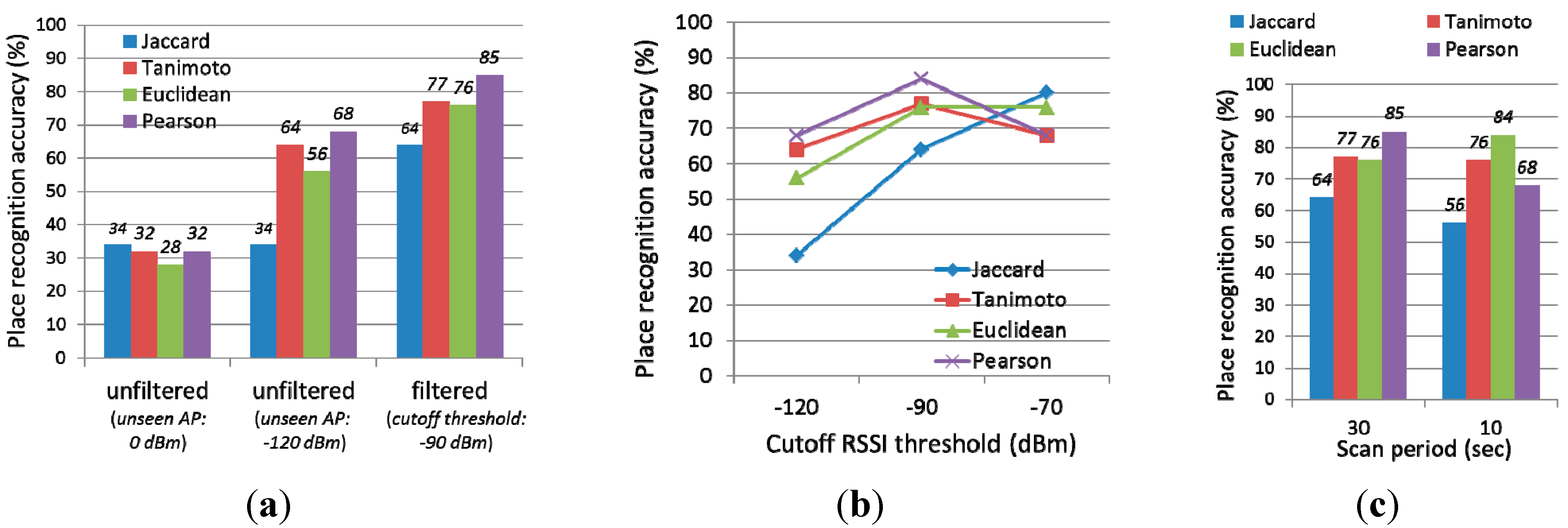
5.1. Place Recognition Accuracy
5.1.1. Data Collection
5.1.2. Evaluation Results

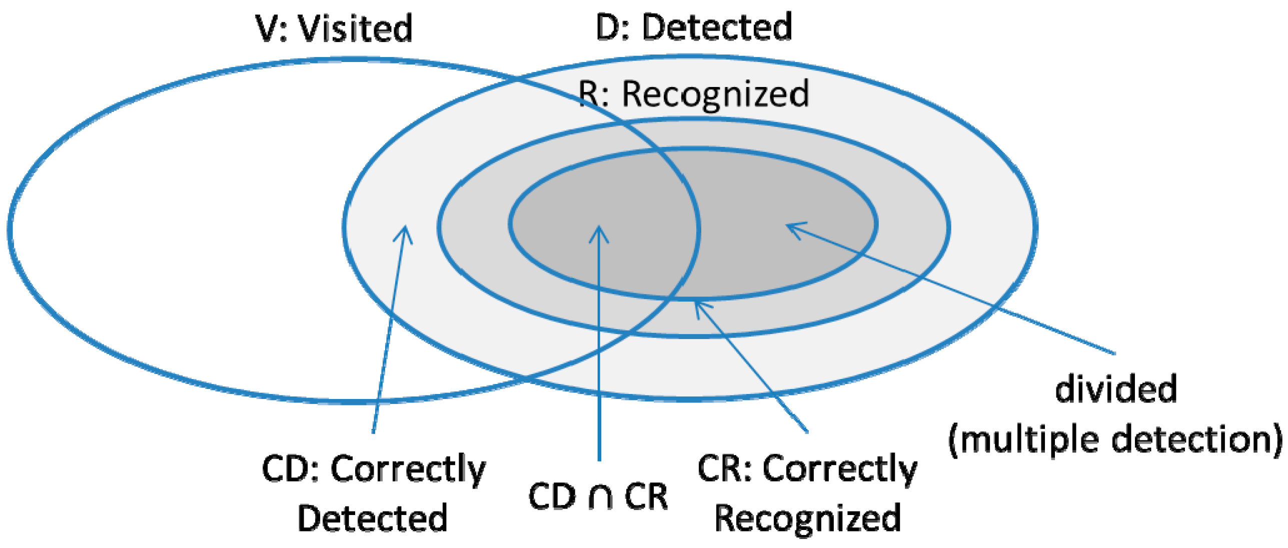
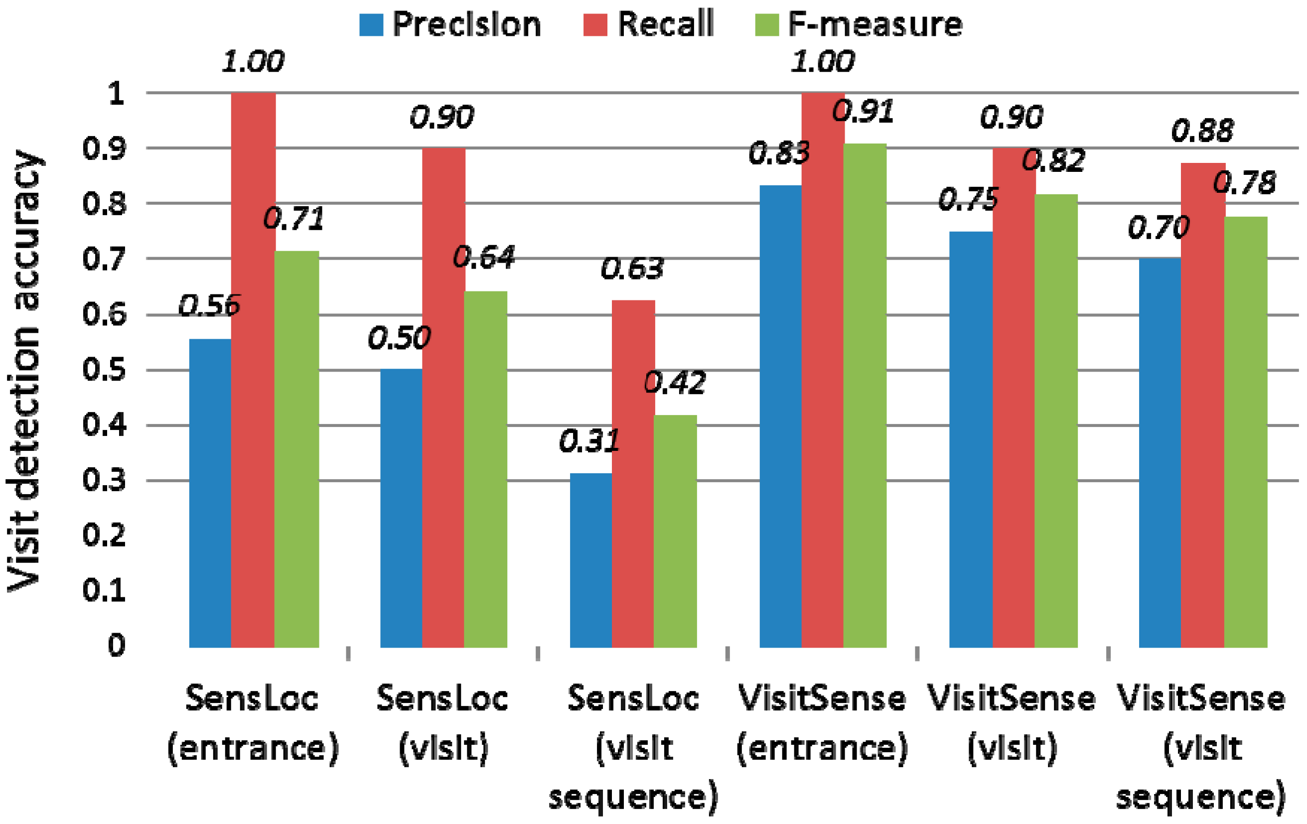
5.2. Visit Detection Accuracy
5.2.1. Data Collection
5.2.2. Methodology

5.2.3. Evaluation Results

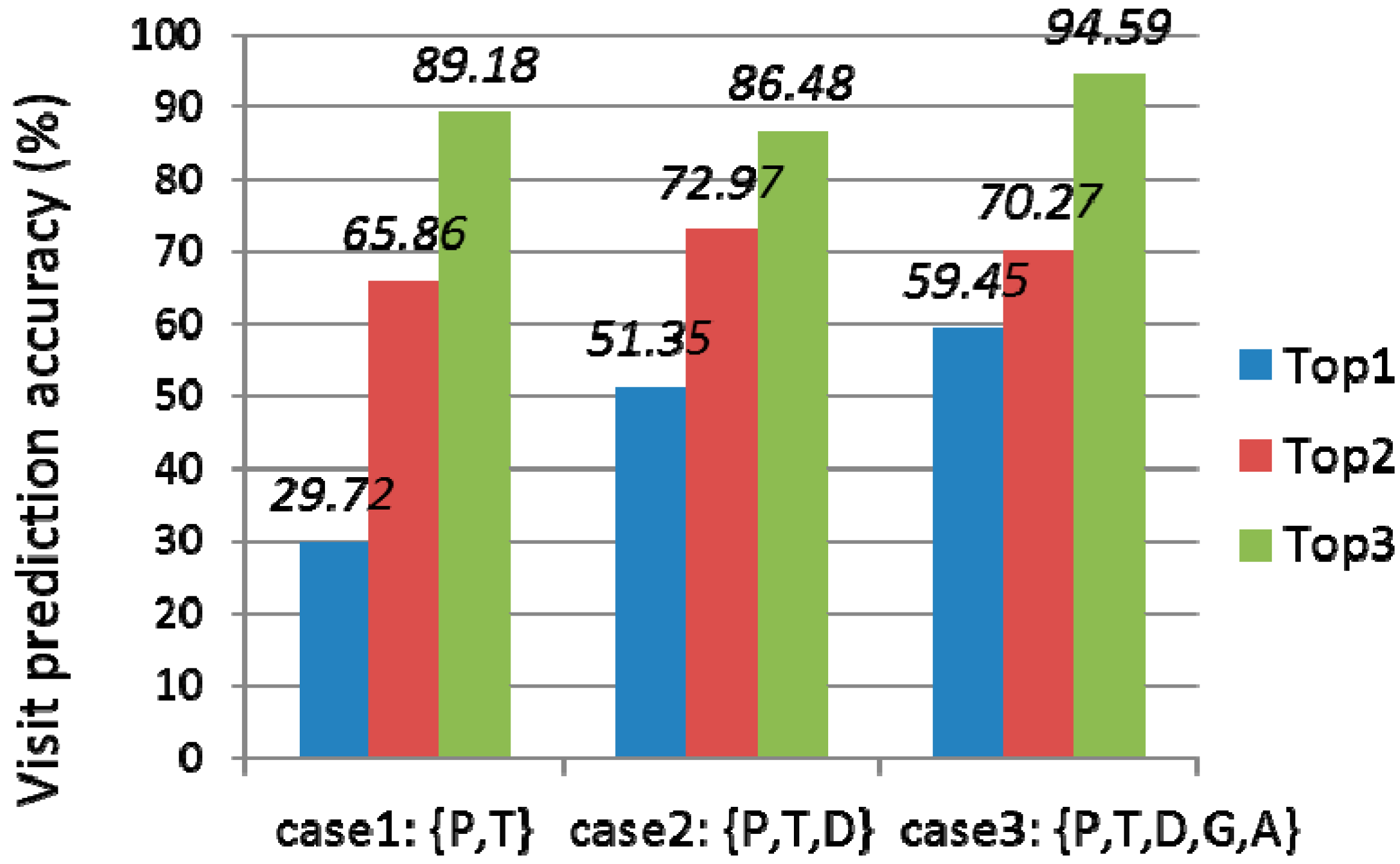
5.3. Visit Prediction Accuracy
5.3.1. Data Collection
| Attribute | Number | Ratio | |
|---|---|---|---|
| Sex | Man | 22 | 29% |
| Woman | 52 | 68% | |
| N/A | 2 | 3% | |
| Age | ~19 | 9 | 12% |
| 20–29 | 48 | 63% | |
| 30–39 | 14 | 18% | |
| 40~ | 2 | 3% | |
| N/A | 3 | 4% | |
| Job | student | 35 | 46% |
| employee | 27 | 36% | |
| others | 7 | 9% | |
| N/A | 7 | 9% | |
| Total | 76 | ||
5.3.2. Evaluation Results

| Classifier | Evaluation Method | Prediction Accuracy (%) | |
|---|---|---|---|
| Structure Learning Algorithm | |||
| Decision tree | N/A | 80% split | 40.54 |
| CRFs | N/A | 80% split | 29.72 |
| Bayesian networks | Domain knowledge | 80% split | 59.45 |
| Repeated Hill Climbing | 80% split | 65 | |
| cross-validation | 52.76 | ||
| Inferred Causation | 80% split | 55 | |
| cross-validation | 51.76 | ||
5.4. Preliminary User Study
5.4.1. Methodology
| Attribute | Number | |
|---|---|---|
| Sex | Man | 7 |
| Woman | 8 | |
| Age | 20–22 | 5 |
| 23–26 | 8 | |
| 27–29 | 2 | |
| Affiliation | KAIST | 8 |
| Others | 7 | |
| Total | 15 | |
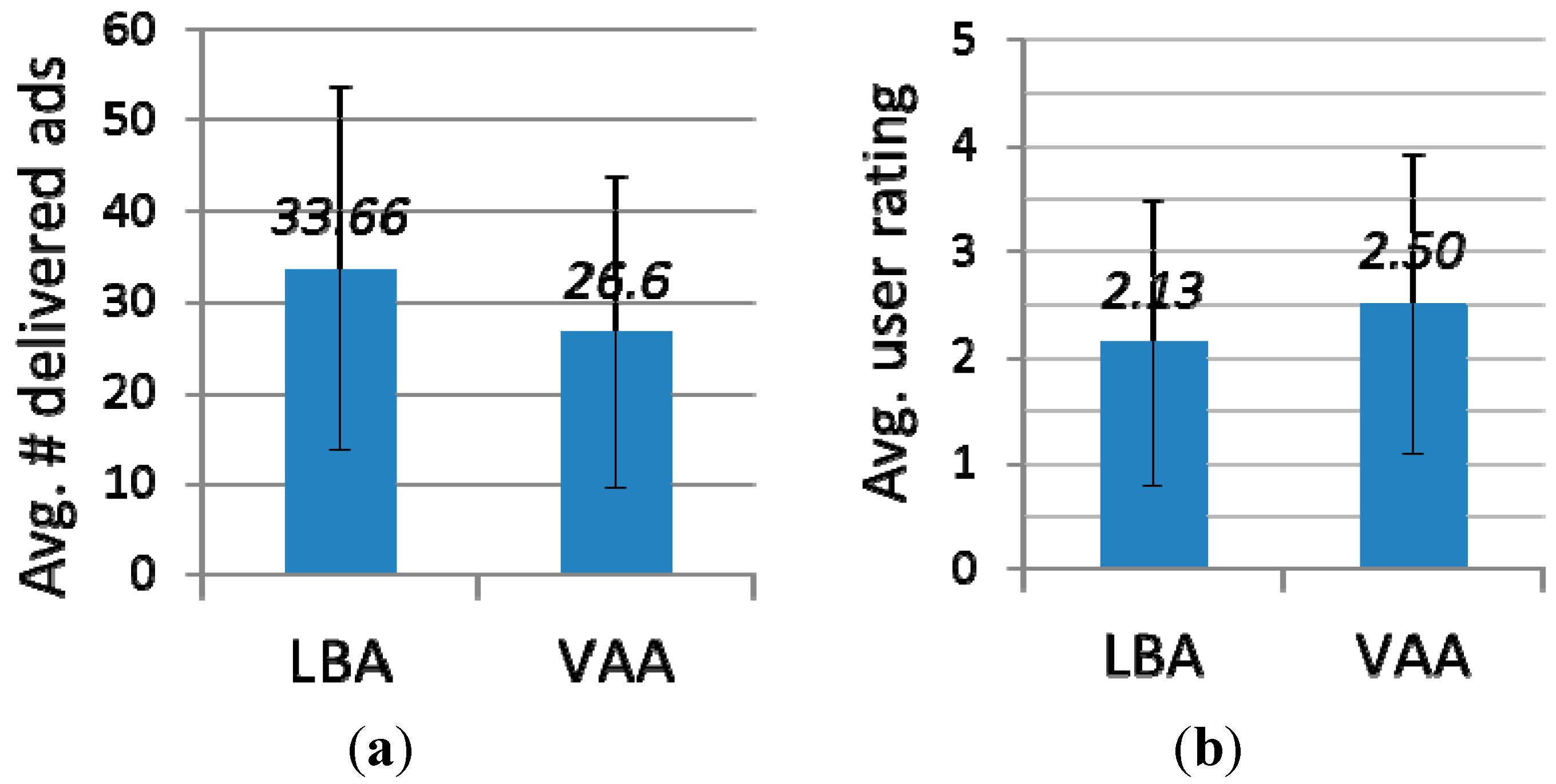
5.4.2. Results

6. Limitation and Discussion
7. Conclusions
Author Contributions
Conflicts of Interest
References
- COEX Mall. Available online: http://www.coexmall.com/index.do (accessed on 21 April 2015).
- Krumm, J. Ubiquitous advertising: The killer applications for the 21th century. IEEE Pervasive Comput. 2010, 10, 66–73. [Google Scholar] [CrossRef]
- Kim, B.; Ha, J.; Lee, S.; Kang, S.; Lee, Y.; Rhee, Y.; Nachman, L.; Song, J. AdNext: A Visit-Pattern-Aware Mobile Advertising System for Urban Commercial Complexes. In Proceedings of the 12th Workshop on Mobile Computing Systems and Applications (HotMobile’11), Phoenix, AZ , USA, 1–3 March 2011.
- Nath, S.; Lin, F.X.; Ravindranath, L.; Padhye, J. SmartAds: Bringing Contextual Ads to Mobile Apps. In Proceedings of the 11th International Conference on Mobile Systems, Applications, and Services (MobiSys’13), Taipei, Taiwan, 25–28 June 2013.
- Alto, L.; Gothlin, N.; Korhonen, J.; Ojala, T. Bluetooth and WAP Push Based Location-Aware Advertising System. In Proceedings of the 2nd International Conference on Mobile Systems, Applications, and Services (MobiSys’04), Boston, MA, USA, 6–9 June 2004.
- Yan, J.; Liu, N.; Wang, G.; Zhang, W.; Jiang, Y.; Chen, Z. How much can Behavioral Targeting Help Online Advertising? In Proceedings of the 18th International Conference on World Wide Web (WWW’09), Madrid, Spain, 20–24 April 2009.
- Hightower, J.; Consolvo, S.; LaMarca, A.; Smith, I.; Hughes, J. Learning and Recognizing the Places We Go. In Proceedings of the 7th International Conference on Ubiquitous Computing (UbiComp’05), Tokyo, Japan, 11–14 September 2005.
- Kim, D.H.; Hightower, J.; Govindan, R.; Estrin, D. Discovering Semantically Meaningful Places from Pervasive RF-beacons. In Proceedings of the 11th International Conference on Ubiquitous Computing (UbiComp’09), Orlando, FL, USA, 30 September–3 October 2009.
- Kim, D.H.; Kim, Y.; Estrin, D.; Srivastava, M.B. SensLoc: Sensing Everyday Places and Paths using Less Energy. In Proceedings of the 8th ACM Conference on Embedded Networked Sensor Systems (SenSys’10), Zurich, Switzerland, 3–5 November 2010.
- Want, R.; Hopper, A.; Falcao, V.; Gibbons, J. The active badge location system. ACM Trans. Inf. Syst. 1992, 40, 91–102. [Google Scholar] [CrossRef]
- Bahl, P.; Padmanabhan, V.N. RADAR: An in-Building RF-Based User Location and Tracking System. In Proceedings of the 19th Annual Joint Conference of the IEEE Computer and Communications Societies (INFOCOM’00), Tel-Aviv, Israel, 26–30 March 2000.
- Zaruba, G.V.; Huber, M.; Kamangar, F.A.; Chlamtac, I. Indoor localization tracking using RSSI readings from a single Wi-Fi access point. Wirel. Netw. 2007, 13, 221–235. [Google Scholar] [CrossRef]
- Yoon, S.; Lee, K.; Rhee, I. FM-Based Indoor Localization via Automatic Fingerprint DB Construction and Matching. In Proceedings of the 11th International Conference on Mobile Systems, Applications, and Services (MobiSys’13), Taipei, Taiwan, 25–28 June 2013.
- Chung, J.; Donahoe, M.; Schmandt, C.; Kim, I.; Razavai, P.; Wiseman, M. Indoor Location Sensing Using Geo-Magnetism. In Proceedings of the 9th International Conference on Mobile Systems, Applications, and Services (MobiSys’11), Washington, DC, USA, 28 June–1 July 2011.
- Park, J.; Charrow, B.; Curtis, D.; Battat, J.; Minkov, E.; Hicks, J.; Teller, S.; Ledlie, J. Growing an Organic Indoor Location System. In Proceedings of the 8th International Conference on Mobile Systems, Applications, and Services (MobiSys’10), San Francisco, CA, USA, 15–18 June 2010.
- Chon, Y.; Lane, N.; Li, F.; Cha, H.; Zhao, F. Automatically Characterizing Places with Opportunistic Crowdsensing using Smartphones. In Proceedings of the 14th International Conference on Ubiquitous Computing (UbiComp’12), Pittsburgh, PA, USA, 5–8 September 2012.
- Morillo, L.M.S.; Ramirez, J.A.O.; Garcia, J.A.A.; Gonzalez-Abril, L. Outdoor exit detection using combined techniques to increase GPS efficiency. Expert Syst. Appl. 2012, 39, 12260–12267. [Google Scholar] [CrossRef]
- Azizyan, M.; Constandache, I.; Choudhury, R.R. SurroundSense: Mobile Phone Localization via Ambience Fingerprinting. In Proceedings of the 15th Annual International Conference on Mobile Computing and Networking (MobiCom’09), Beijing, China, 20–25 September 2009.
- Song, C.; Qu, Z.; Blumm, N.; Barabasi, A.-L. Limits of predictability in human mobility. Science 2010, 327, 1018–1021. [Google Scholar] [CrossRef] [PubMed]
- Ashbrook, D.; Starner, T. Using GPS to learn significant locations and predict movement across multiple users. Pers. Ubiquitous Comput. 2003, 7, 275–286. [Google Scholar] [CrossRef]
- Patterson, D.J.; Liao, L.; Fox, D.; Kautz, H. Inferring High-Level Behavior from Low-Level Sensors. In Proceedings of the 5th International Conference on Ubiquitous Computing (UbiComp’03), Seattle, WA, USA, 12–15 October 2003.
- Liao, L.; Fox, D.; Kautz, H. Location-Based Activity Recognition using Relational Markov Networks. In Proceedings of the 19th International Joint Conferences on Artificial Intelligence (IJCAI’05), Edinburgh, Scotland, UK, 31 July–5 August 2005.
- Kjarulff, U.B.; Madsen, A.L. Bayesian Networks and Influence Diagrams: A Guide to Construction and Analysis. In Information Science and Statistics; Springer-Verlag: New York, NY, USA, 2008. [Google Scholar]
- Dempster, A.P.; Laird, N.M.; Rubin, D.B. Maximum likelihood from incomplete data via the EM algorithm. J. R. Stat. Soc. (JSTOR) 1977, 39, 1–38. [Google Scholar]
- Druzdzel, M.J. SMILE: Structural Modeling, Inference, and Learning Engine and GeNIe: A Development Environment for Graphical Decision-Theoretic Models. In Proceedings of the 16th National Conference on Artificial Intelligence and the 11th Conference on Innovative Applications of Artificial Intelligence (AAAI’99/IAAI’99), Orlando, FL, USA, 18–22 July 1999.
- Weka 3. Available online: http://www.cs.waikato.ac.nz/ml/weka/ (accessed on 21 April 2015).
- CRF Software Package. Available online: http://crf.sourceforge.net (accessed on 21 April 2015).
- Buntine, W. A guide to the literature on learning probabilistic networks from data. IEEE Trans. Knowl. Data Eng. (TKDE) 1996, 8, 195–210. [Google Scholar] [CrossRef]
- Verma, T.; Pearl, J. An Algorithm for Deciding if a Set of Observed Independencies has a Causal Explanation. In Proceedings of the 8th Annual Conference on Uncertainty in Artificial Intelligence (UAI’92), Stanford, CA, USA, 17–19 July 1992.
- Shoppers Would Rather Use Smartphones than Consult Store Associates, Survey Finds. Available online: https://www.internetretailer.com/2010/12/06/shoppers-would-rather-use-smartphones-store-associates (accessed on 17 June 2015).
- Hipcricket: Mobile Shoppers Buying Because of Mobile Ads. Available online: http://www.bizreport.com/2012/07/hipcricket-mobile-shoppers-buying-because-of-mobile-ads.html (accessed on 17 June 2015).
- Sen, R.; Lee, Y.; Jayarajah, K.; Misra, A.; Balan, R.K. GruMon: Fast and accurate group monitoring for heterogeneous urban spaces. In Proceedings of the 12th ACM Conference on Embedded Network Sensor Systems (SenSys’14), Memphis, TN, USA, 3–6 November 2014.
© 2015 by the authors; licensee MDPI, Basel, Switzerland. This article is an open access article distributed under the terms and conditions of the Creative Commons Attribution license (http://creativecommons.org/licenses/by/4.0/).
Share and Cite
Kim, B.; Kang, S.; Ha, J.-Y.; Song, J. VisitSense: Sensing Place Visit Patterns from Ambient Radio on Smartphones for Targeted Mobile Ads in Shopping Malls. Sensors 2015, 15, 17274-17299. https://0-doi-org.brum.beds.ac.uk/10.3390/s150717274
Kim B, Kang S, Ha J-Y, Song J. VisitSense: Sensing Place Visit Patterns from Ambient Radio on Smartphones for Targeted Mobile Ads in Shopping Malls. Sensors. 2015; 15(7):17274-17299. https://0-doi-org.brum.beds.ac.uk/10.3390/s150717274
Chicago/Turabian StyleKim, Byoungjip, Seungwoo Kang, Jin-Young Ha, and Junehwa Song. 2015. "VisitSense: Sensing Place Visit Patterns from Ambient Radio on Smartphones for Targeted Mobile Ads in Shopping Malls" Sensors 15, no. 7: 17274-17299. https://0-doi-org.brum.beds.ac.uk/10.3390/s150717274