
A Method for Oscillation Errors Restriction of SINS Based on Forecasted Time Series

Abstract
:1. Introduction

2. Analysis of Periodic Oscillation Errors of SINS
3. Method for Oscillation Errors Restriction Based on Forecasted Time Series
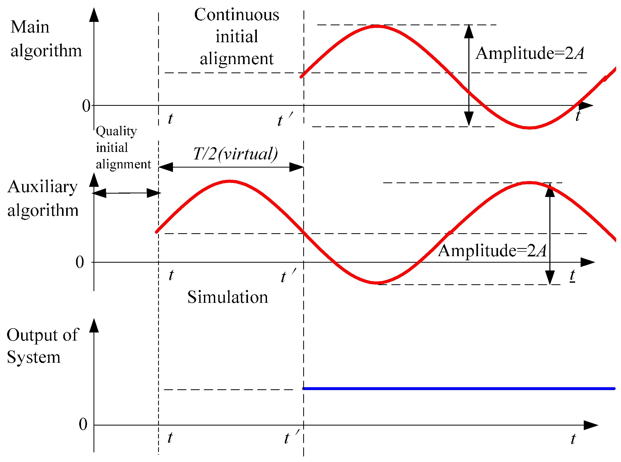
3.1. Principle of Eliminating Periodic Oscillation Signal with Half-Wave Delay by Mean Value
3.2. Method for Oscillation Errors Restriction Based on Forecasted Time Series

4. Method for Obtaining Forecasted Time Series by Curve Fitting Based on Least Square Method
4.1. Curve Fitting Based on Least Square Method
4.2. Problem Description

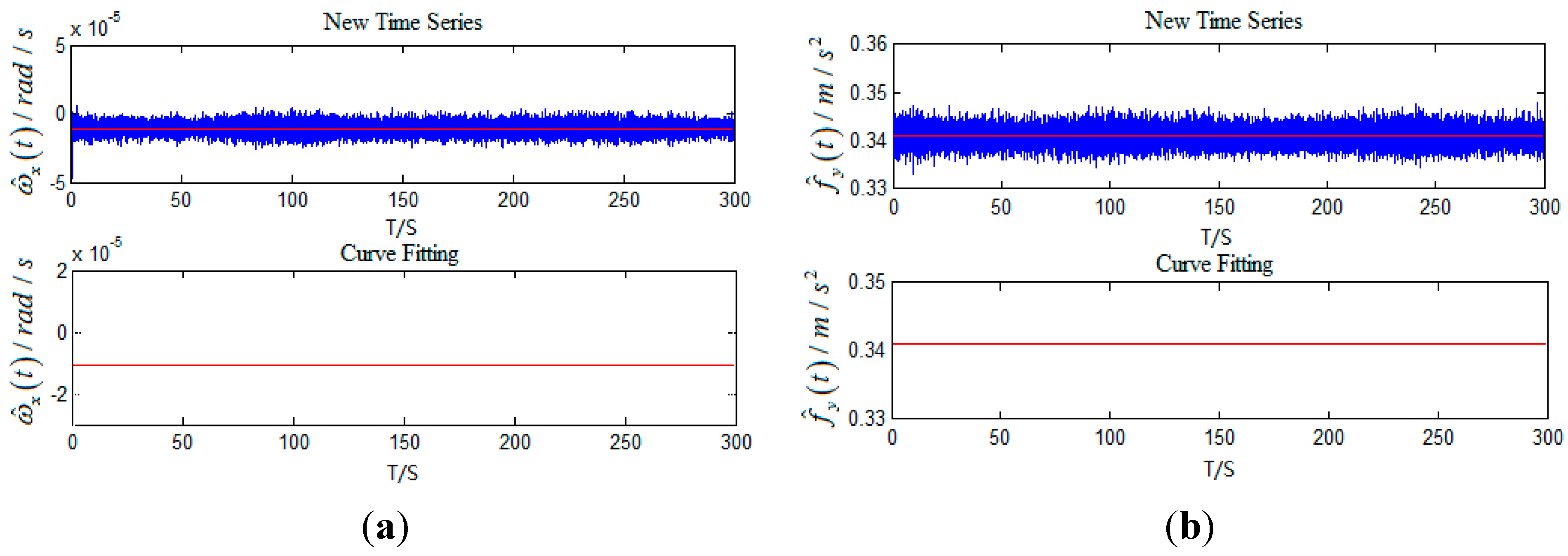
4.3. Forecasted Time series Obtained by Curve Fitting Based on Least Square Method


5. Computer Simulations
5.1. Simulation of Maneuvering Carrier
5.1.1. Simulation with No Inertia Device Errors


5.1.2. Simulation with Inertia Device Errors

6. System Test
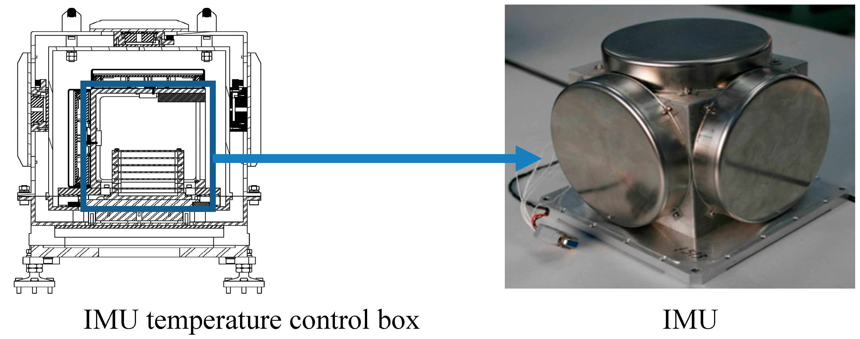
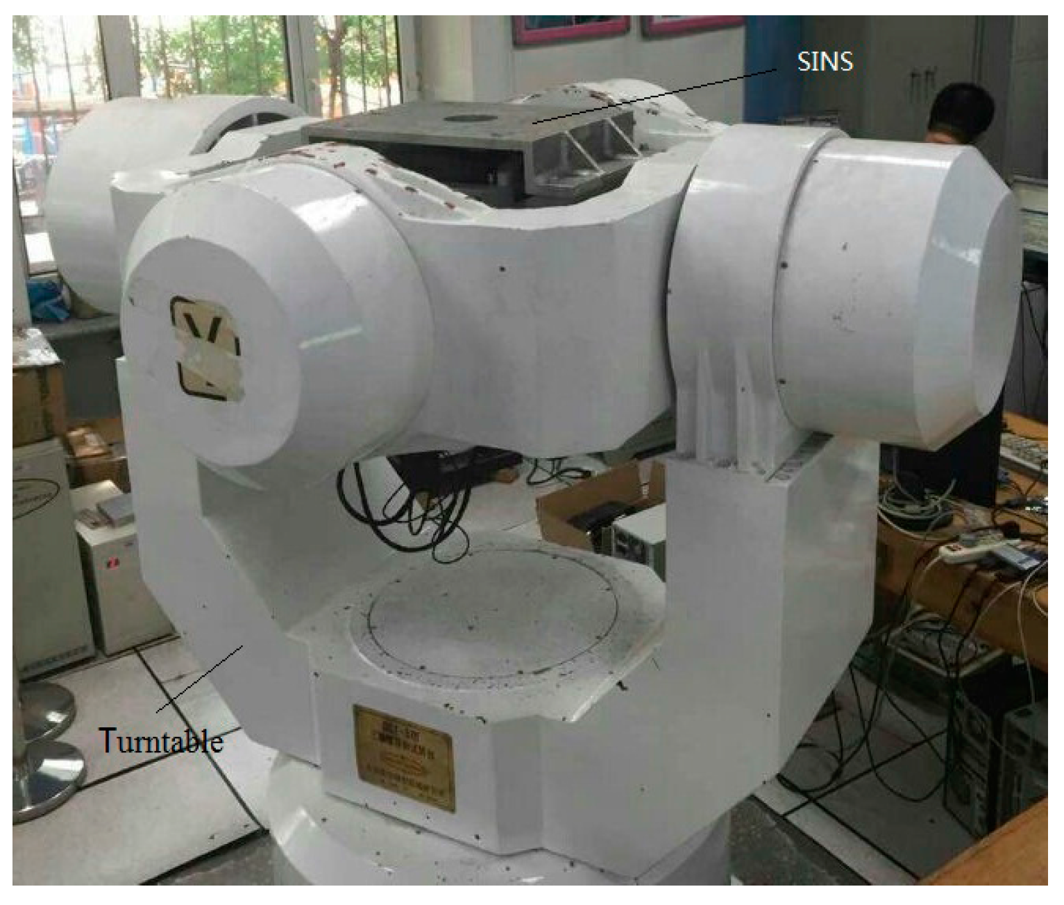
6.1. Test Equipment


6.2. Test
6.2.1. Test Preparation
6.2.2. Test Process
6.2.3. Test Set
6.2.4. Sampling Frequency and Update Frequency
6.2.5. Reference Datum
6.2.6. Initial Attitude Errors
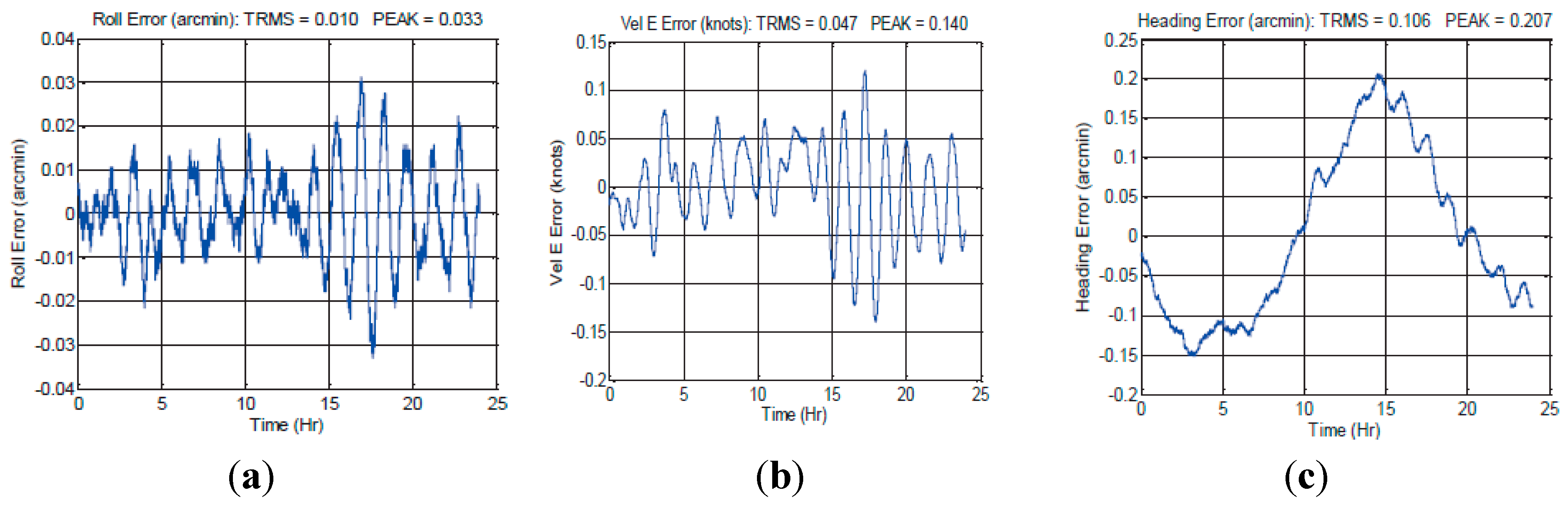
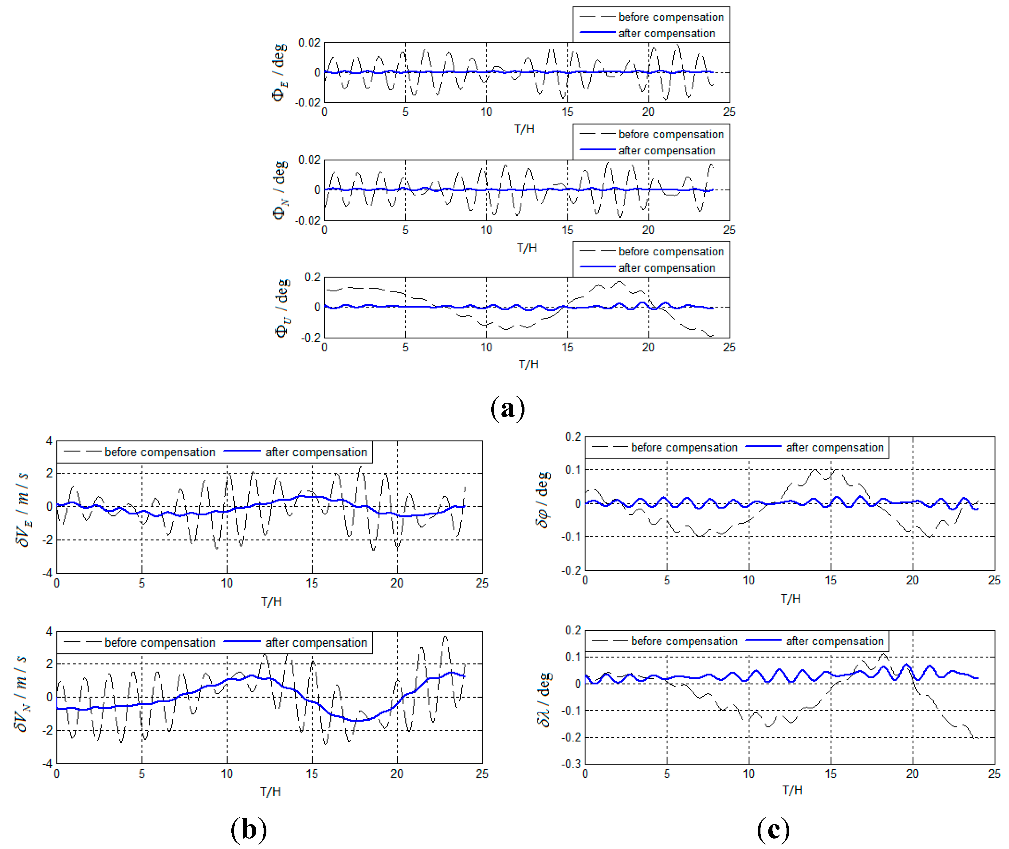
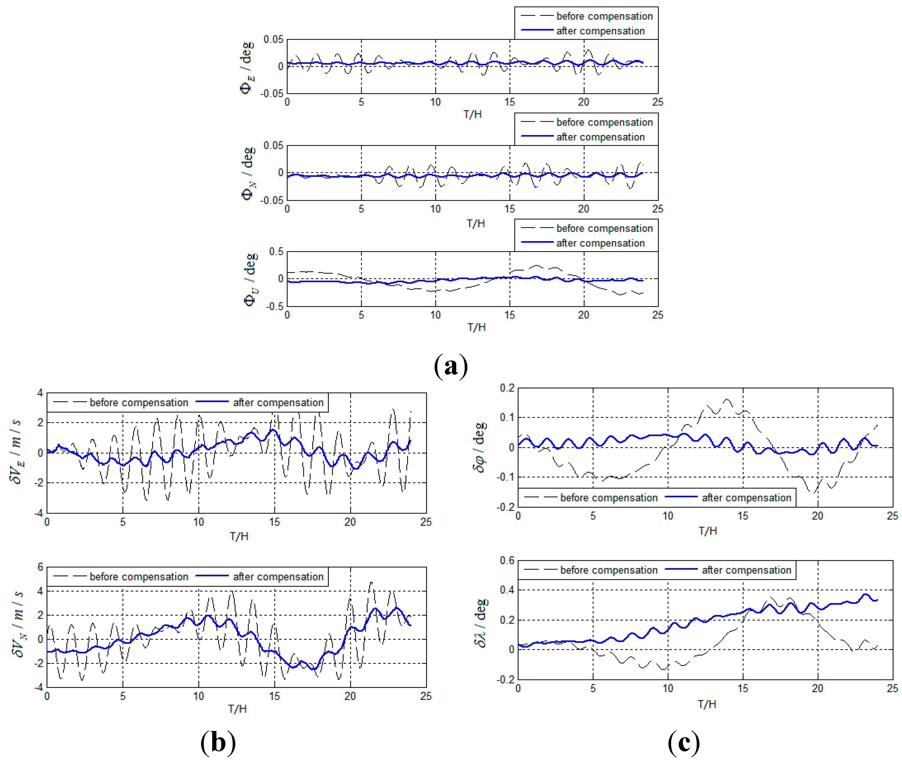
6.3. Test Results

7. Conclusions
Acknowledgments
Author Contributions
Conflicts of Interest
References
- Tazartes, D.A. Inertial Navigation: From Gimbaled Platforms to Strapdown Sensors. IEEE Trans. Aerosp. Electron. Syst. 2011, 47, 2292–2299. [Google Scholar]
- Malakar, B.; Roy, B. A novel application of adaptive filtering for initial alignment of strapdown inertial navigation system. In Proceedings of the 2014 International Conference on Circuits, Systems, Communication and Information Technology Applications (CSCITA), Mumbai, India, 4–5 April 2014; pp. 189–194.
- Vajda, S.; Zom, A. Survey of existing and emerging technologies for strategic submarine navigation. In Proceedings of the IEEE Position Location and Navigation, Symposium, Palm Springs, CA, USA, 20–23 April 1998; pp. 309–315.
- Acharya, A.; Sadhu, S.; Ghoshal, T.K. Improving Self-Alignment of Strapdown INS Using Measurement Augmentation. In Proceedings of the 12th International Conference on Information Fusion, Seattle, WA, USA, 6–9 July 2009; pp. 1783–1789.
- Ma, Y.; Fang, J.; Wang, W. Decoupled Observability Analyses of Error States in INS/GPS Integration. J. Navig. 2014, 67, 473–494. [Google Scholar] [CrossRef]
- Zheng, Z.; Yue, J. A Novel GPS/INS Loose Integrated Navigation Algorithm. Adv. Mater. Res. 2013, 823, 479–484. [Google Scholar] [CrossRef]
- Kevin, C.; Robert, G.; Marvin, B.M.; Scott, G. Navy Testing of the iXBlue MARINS Fiber Optic Gyroscope (FOG) Inertial Navigation System (INS). In Proceedings of IEEE/ION Position, Location and Navigation Symposium-PLANS, Monterey, CA, USA, 5–8 May 2014; pp. 1392–1408.
- Tawk, Y.; Tomé, P.; Botteron, C.; Stebler, Y.; Farine, P.A. Implementation and Performance of a GPS/INS Tightly Coupled Assisted PLL Architecture Using MEMS Inertial Sensors. Sensors 2014, 14, 3768–3796. [Google Scholar] [CrossRef] [PubMed]
- Gao, W.; Zhang, Y.; Wang, J. A Strapdown Interial Navigation System/Beidou/Doppler Velocity Log Integrated Navigation Algorithm Based on a Cubature Kalman Filter. Sensors 2014, 14, 1511–1527. [Google Scholar] [CrossRef] [PubMed]
- Chen, J.; Zou, J.; Wu, L.; Hao, Y.; Gan, S. The Design of an Effective Marine Inertial Navigation System Scheme. In Proceedings of the International Workshop on Knowledge Discovery and Data Mining (WKDD 2008), Adelaide, Australia, 23–24 January 2008; pp. 671–676.
- Grammatikos, A.; Schuler, A.R.; Fegley, K.A. Damping gimballess inertial navigation system. IEEE Trans. Aerosp. Electron. Syst. 1967, 3, 481–493. [Google Scholar] [CrossRef]
- Hao, Y.; Gong, J.; Gao, W.; Li, L. Research on the dynamic error of strapdown inertial navigation system. In Proceedings of the IEEE International Conference on Mechatronics and Automation, 2008 (ICMA 2008), Takamatsu, Japan, 5–8 August 2008; pp. 814–819.
- Xu, B.; Sun, F. An independent damped algorithm based on SINS for ship. In Proceedings of 2009 International Conference on Computer Engineering and Technology, Singapore, Singapore, 22–24 January 2009; pp. 88–92.
- Gao, W.; Zhang, Y. Analyses of Damping Network Effect on SINS. In Proceedings of the International Conference on Mechatronics and Automation, Changchun, China, 9–12, August 2009; pp. 2530–2535.
- Ra, W.S.; Whang, I.H.; Park, H.R. Robust damping loop design for GPS/INS vertical channel. Electron. Lett. 2006, 42, 617–618. [Google Scholar] [CrossRef]
- Huang, W.Q.; Hao, Y.L.; Cheng, J.H.; Li, G.; Fu, I.G.; Bu, X.B. Rearch of the inertial navigation system with variable damping coefficients horizontal damping networks. In Proceedings of Oceans’ 04 MTS /IEEE Techno-Ocean’ 04 Conference, Kobe, Japan, 9–12 November 2004; pp. 1272–1276.
- Gao, W.; Zhang, Y.; Ben, Y.; Sun, Q. An Automatic Compensation Method for States Switch of Strapdown Inertial Navigation System. In Proceedings of IEEE/ION Position Location and Navigation Symposium, Myrtle Beach, SC, USA, 23–26 April 2012; pp. 814–817.
- Tucker, T.; Levinson, E. The AN/WSN-7B marine gyrocompass/navigator. In Proceedings of the 2000 National Technical Meeting of the Institute of Navigation, Anaheim, CA, USA, 26–28 January 2000; pp. 348–357.
- Du, Y.; Liu, J.; Liu, R.; Zhu, Y. The fuzzy Kalman filtering of damp attitude algorithm. J. Astronaut. 2007, 28, 305–309. [Google Scholar]
- Ma, X.J.; Liu, H.W.; Xiao, D.; Li, H.K. Key technologies of geomagnetic aided inertial navigation system. In Proceedings of the IEEE Intelligent Vehicles Symposium, Xi’an, China, 3–5 June 2009; pp. 464–469.
- Jaradat, M.A.K.; Abdel-Hafez, M.F. Enhanced, Delay Dependent, Intelligent Fusion for INS/GPS Navigation System. IEEE Sens. J. 2014, 14, 1545–1554. [Google Scholar] [CrossRef]
- Adusumilli, S.; Bhatt, D.; Wang, H.; Bhattacharya, P.; Devabhaktuni, V. A low-cost INS/GPS integration methodology based on random forest regression. Expert Syst. Appl. 2013, 40, 4653–4659. [Google Scholar] [CrossRef]
- Lee, J.K.; Jekeli, C. Neural Network Aided Adaptive Filtering and Smoothing for an Integrated INS/GPS Unexploded Ordnance Geolocation System. J. Navig. 2010, 63, 251–267. [Google Scholar] [CrossRef]
- Nassar, S.; El-Sheimy, N. A combined algorithm of improving INS error modeling and sensor measurements for accurate INS/GPS navigation. GPS Solut. 2006, 10, 29–39. [Google Scholar] [CrossRef]
- Musavi, N.; Keighobadi, J. Adaptive fuzzy neuro-observer applied to low cost INS/GPS. Appl. Soft Comput. 2015, 29, 82–94. [Google Scholar] [CrossRef]
- Gonzalez, R.; Giribet, J.I.; Patino, H.D. An approach to benchmarking of loosely coupled low-cost navigation systems. Math. Comput. Model. Dyn. Syst. 2015, 21, 272–287. [Google Scholar] [CrossRef]
- Welker, T.C.; Pachter, M.; Huffman, R.E. Gravity Gradiometer Integrated Inertial Navigation. In Proceedings of European Control Conference, Zurich, Switzerland, 17–19 July 2013; pp. 846–851.
- Hong, S.P.; Lee, M.H.; Chun, H.H.; Kwon, S.H.; Speyer, J.L. Observability of error states in GPS/INS integration. IEEE Trans. Veh. Technol. 2005, 54, 731–743. [Google Scholar] [CrossRef]
- Yang, Y.; Zhou, J.; Nies, H.; Loffeld, O.; Knedlik, S. Development of a Deeply-Coupled GPS/INS Integration Algorithm Using Quaternions. In Proceedings of 16th International Conference on Information Fusion, Istanbul, Turkey, 9–12 July 2013; pp. 1791–1796.
- Babu, R.; Wang, J.L. Ultra-tight GPS/INS/PL integration: A system concept and performance analysis. GPS Solut. 2009, 13, 75–82. [Google Scholar] [CrossRef]
- Leung, K.T.; Whidborne, J.F.; Purdy, D.; Dunoyer, A. A review of ground vehicle dynamic state estimations utilising GPS/INS. Veh. Syst. Dyn. 2011, 49, 29–58. [Google Scholar] [CrossRef]
© 2015 by the authors; licensee MDPI, Basel, Switzerland. This article is an open access article distributed under the terms and conditions of the Creative Commons Attribution license (http://creativecommons.org/licenses/by/4.0/).
Share and Cite
Zhao, L.; Li, J.; Cheng, J.; Jia, C.; Wang, Q. A Method for Oscillation Errors Restriction of SINS Based on Forecasted Time Series. Sensors 2015, 15, 17433-17452. https://0-doi-org.brum.beds.ac.uk/10.3390/s150717433
Zhao L, Li J, Cheng J, Jia C, Wang Q. A Method for Oscillation Errors Restriction of SINS Based on Forecasted Time Series. Sensors. 2015; 15(7):17433-17452. https://0-doi-org.brum.beds.ac.uk/10.3390/s150717433
Chicago/Turabian StyleZhao, Lin, Jiushun Li, Jianhua Cheng, Chun Jia, and Qiufan Wang. 2015. "A Method for Oscillation Errors Restriction of SINS Based on Forecasted Time Series" Sensors 15, no. 7: 17433-17452. https://0-doi-org.brum.beds.ac.uk/10.3390/s150717433