
Extracting Objects for Aerial Manipulation on UAVs Using Low Cost Stereo Sensors


Abstract
:1. Introduction
2. Methodology
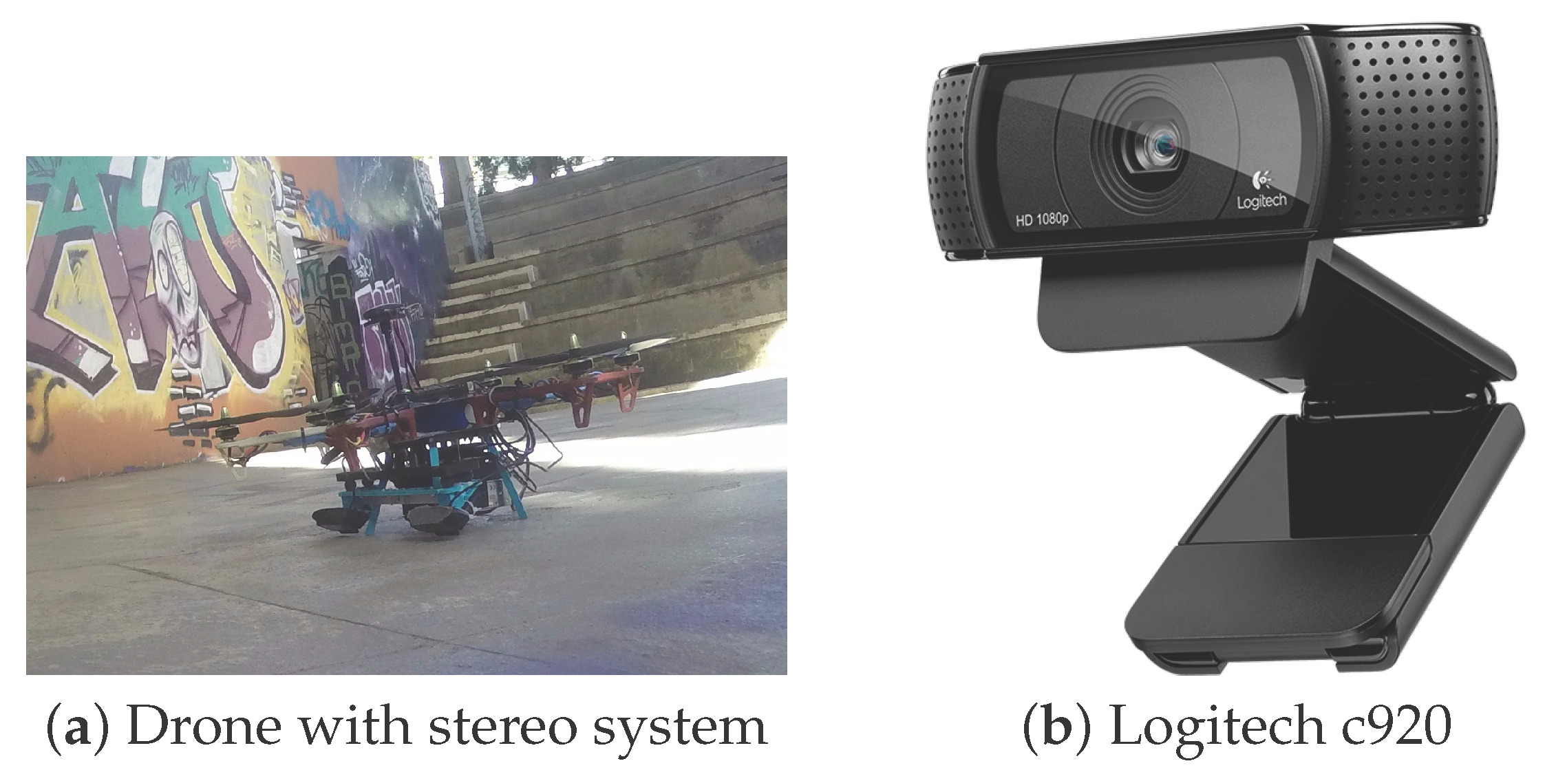
2.1. System Description
2.2. Data Acquisition
- Stereo cameras.
- Inercial measure unit (IMU) module with compass data (Accelerometer, Gyroscope).
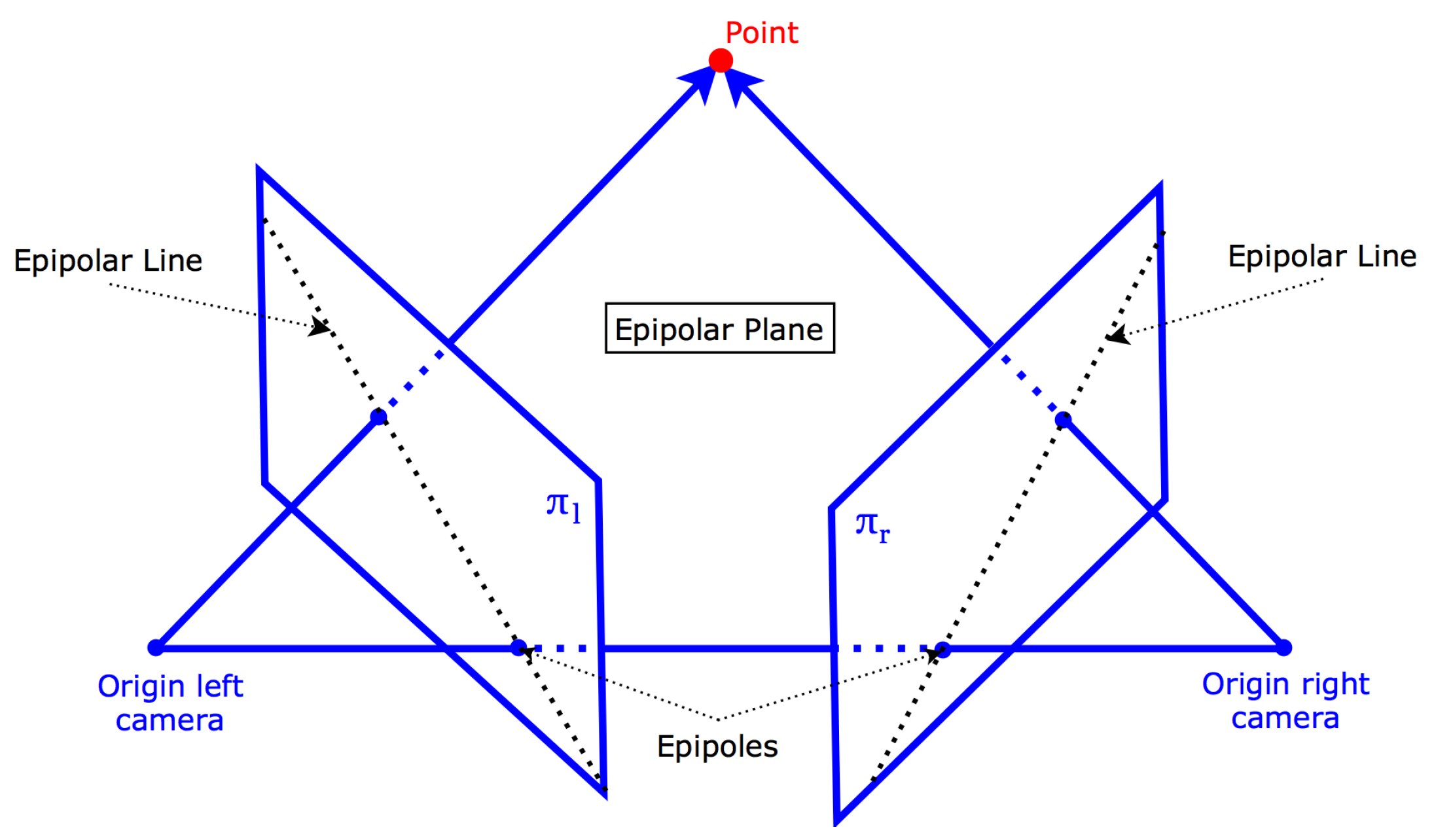
2.3. Point Cloud Generation
- Visual feature detection in the left image.
- Template matching in the right image.
- Triangulation.
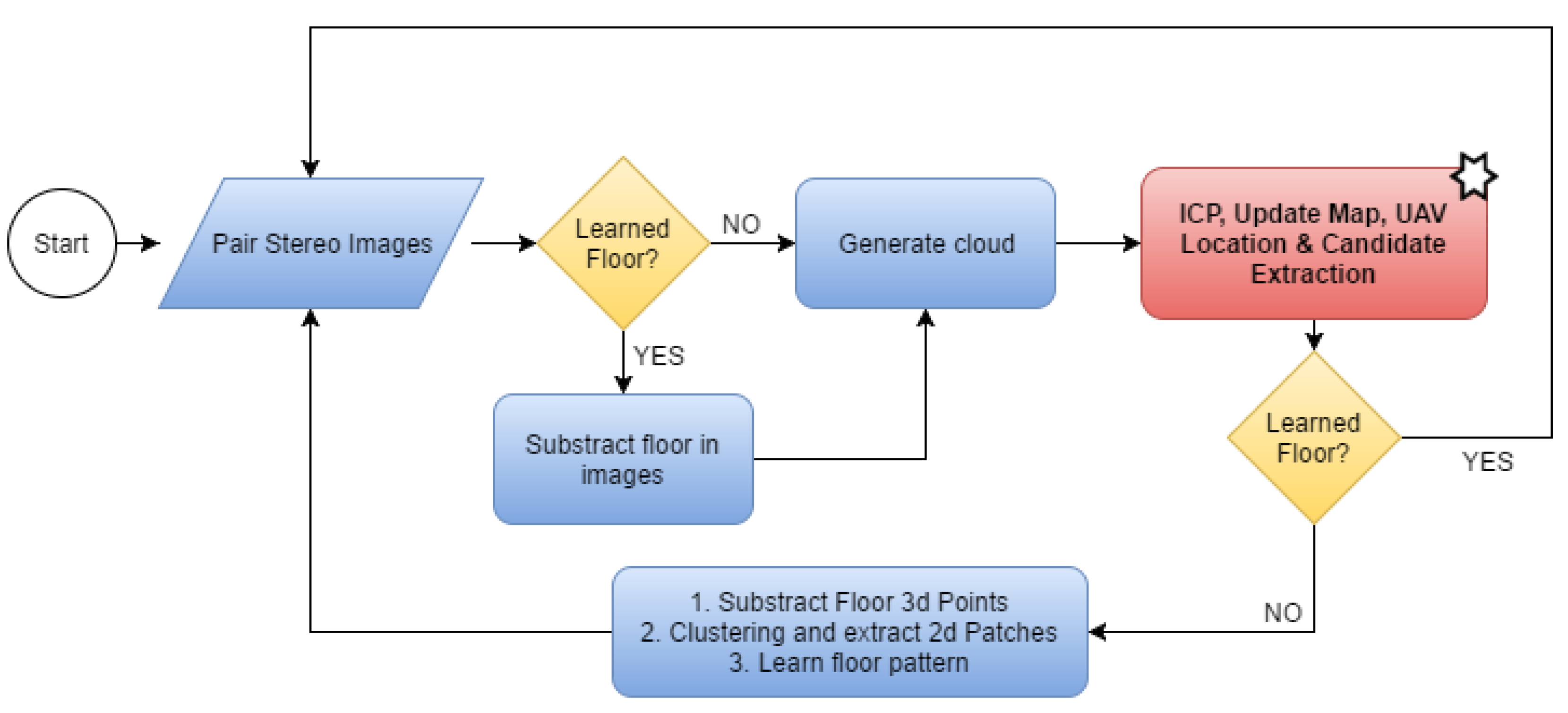
2.4. Floor Detection and Extraction
- The floor in the scene is uniform so it has few features on it.
- The floor has a texture that can be modeled/learned.
- The floor has a texture that cannot be learned.
2.5. Temporal Convolution Voxel Filtering for Map Generation
| Algorithm 1 Probabilistic Map Generation. |
|
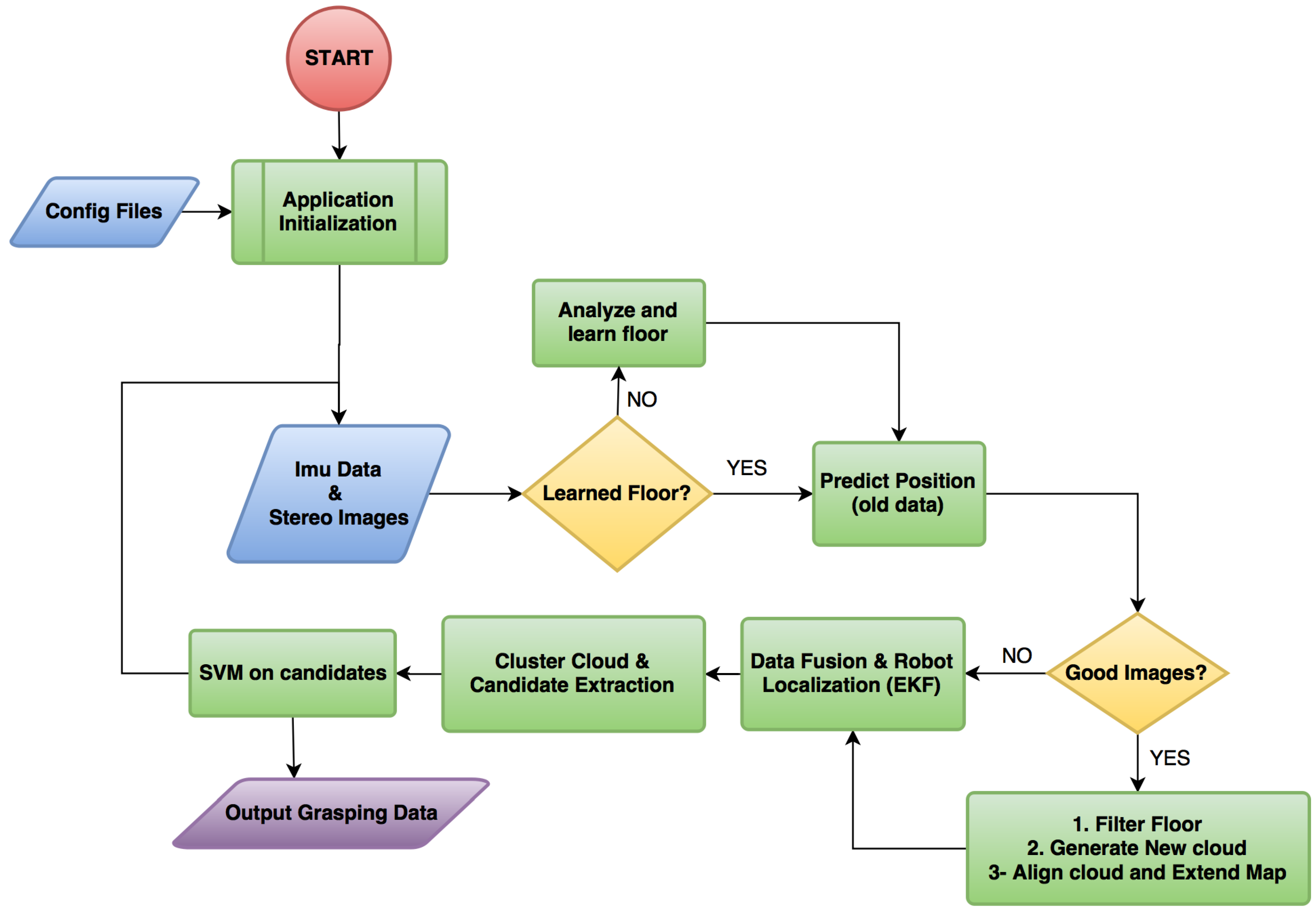
2.6. Drone Positioning and Cloud Alignment
- The previous state is used to obtain , which is a rough estimation of the current position of the robot.
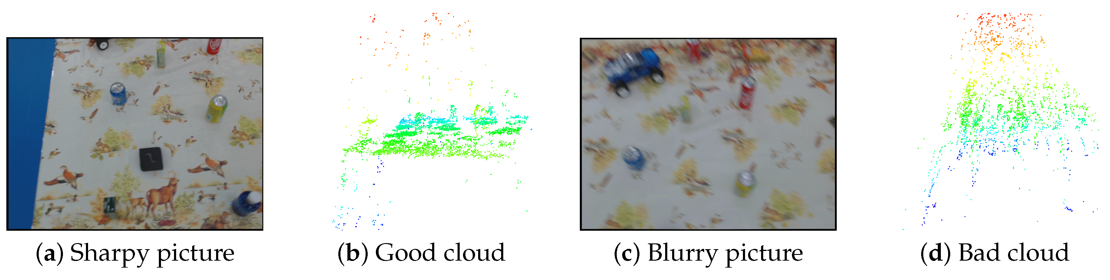
- If the stereo system has captured good images, a point cloud is generated and aligned with the map using as the initial guess. The transformation result of the alignment is used as the true position of the drone . The obtained transformation is compared to the provided guess and discarded, if the difference exceeds a predefined threshold.
- If the stereo system has not captured good images, it is assumed that is a good approximation of the state, so
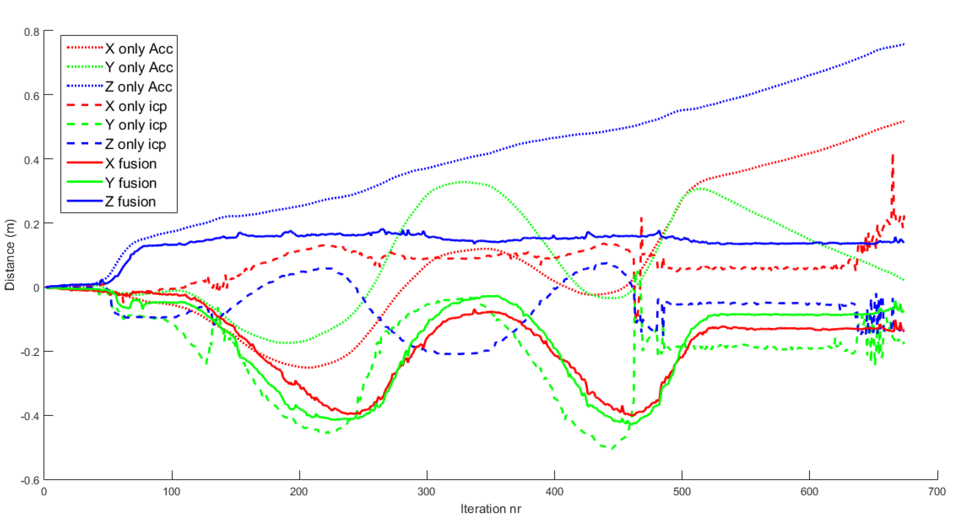
- The EKF merges the information from the ICP , with the information from the IMU, , and the resulting is the current filtered state.
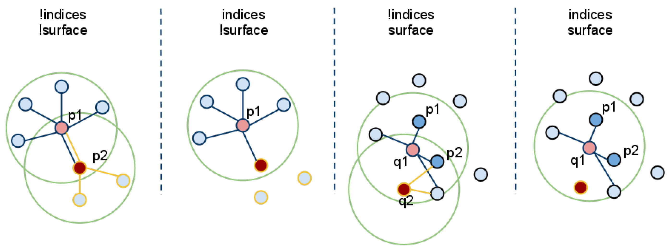
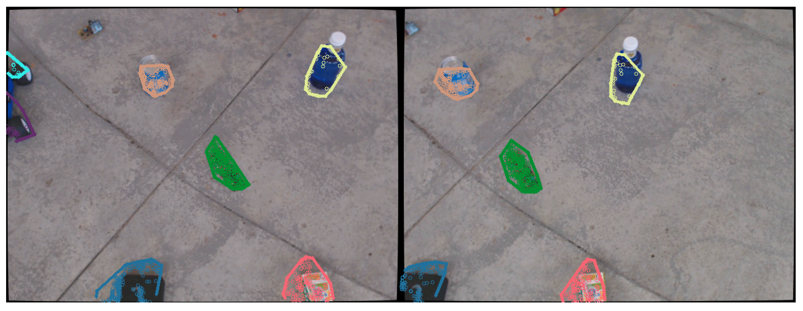
2.7. Candidate Selection
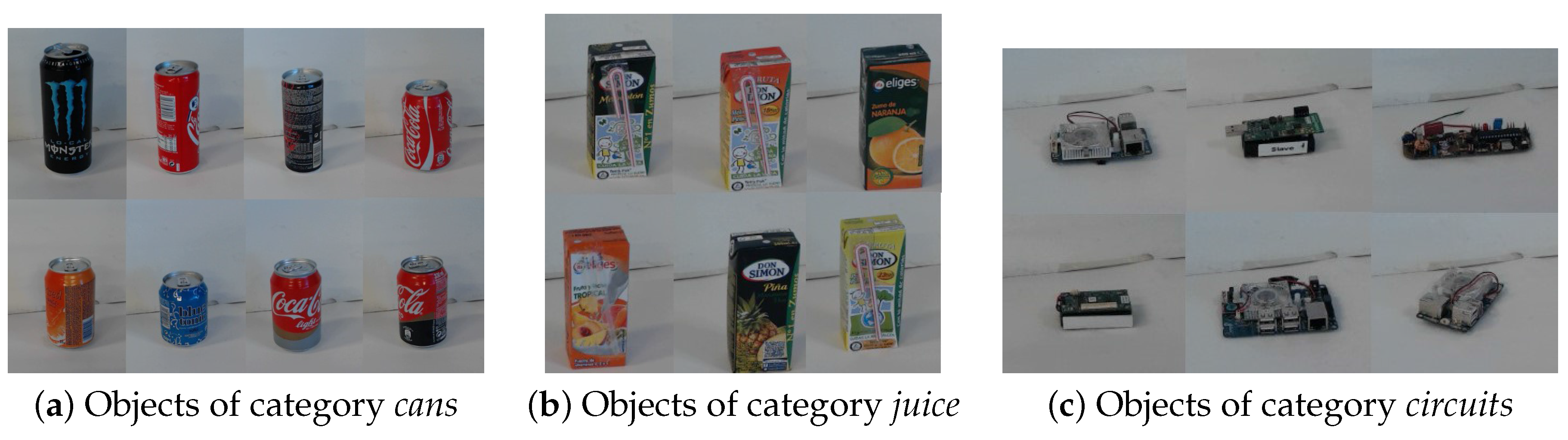
2.8. Object Recognition
2.9. Grasping Data
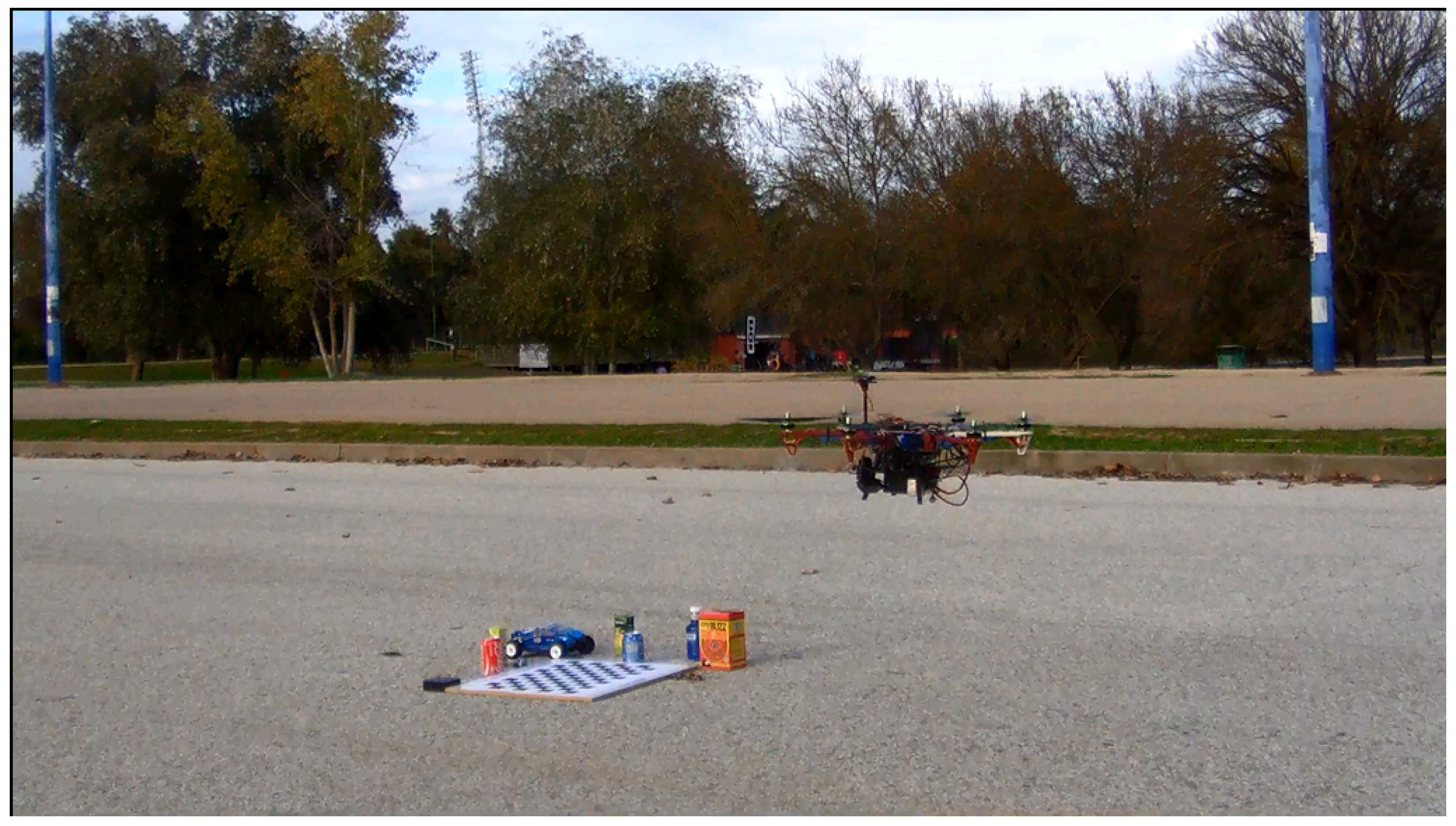
3. Experimental Validation
4. Conclusions
Acknowledgments
Author Contributions
Conflicts of Interest
Appendix A. Parameters of the System
| Parameter | Description | Value |
| Camera Parameters | ||
| ROI | Usable part of images due to distortion | |
| Blur Threshold | Max. value of blurriness (Section 2.2) | – |
| Disparity Range | Min-max distances between pair of pixels. This value determine the min-max distances | px → m |
| Template Square Size | Size of the template for template matching | 7–15 |
| Max Template Score | Max. allowed score of template matching | – |
| Map Generation Parameters | ||
| Voxel Size | Size of voxel in 3D space grid | – |
| Outlier Mean K | Outlier removal parameter | 10–20 |
| Outier Std Dev | Outlier removal parameter | – |
| ICP max epsilon | Max. allowed error in transformation between iterations in ICP | |
| ICP max iterations | Number of iterations of ICP | 10–50 |
| ICP max corresp. dist | Max. initial distance for correspondences | – |
| ICP max fitting Score | Max. score to reject ICP result | – |
| Max allowed Translation | Max. translation to reject ICP result | – |
| Max allowed rotation | Max rotation to reject ICP result | 10–20 |
| History Size | History size of TCVF | 2–4 |
| Cluster Affil. Max. Dist. | Minimal distance between objects | |
| EKF Parameters | ||
| Acc Bias Calibration | Bias data from IMU X,Y,Z | −0.14, 0.051, 6.935 |
| Acc Frequency | Mean frequency of data | 1 KHz |
| Gyro Noise | Average magnitude of noise | |
| Gyro Frequency | Mean frequency of data | 30 KHz |
| Imu to cam Calibration | Transformation between camera and IMU | Data from Calib |
| Q System cov. Mat. | Covariance of System state variables | Data from Calib |
| R Observation cov. Mat. | Covariance of Data | Data from Calib |
| Recognition System | ||
| Training params | Train parameters of SVM | —- |
| Detector Descriptor | Feature detector and descriptor used | SIFT |
References
- Pajares, G. Overview and Current Status of Remote Sensing Applications Based on Unmanned Aerial Vehicles (UAVs). Photogramm. Eng. Remote Sens. 2015, 81, 281–329. [Google Scholar] [CrossRef]
- Budiyanto, A.; Cahyadi, A.; Adji, T.; Wahyunggoro, O. UAV obstacle avoidance using potential field under dynamic environment. In Proceedings of the International Conference on Control, Electronics, Renewable Energy and Communications, Bandung, Indonesia, 27–29 August 2015; pp. 187–192.
- Santos, M.; Santana, L.; Brandao, A.; Sarcinelli-Filho, M. UAV obstacle avoidance using RGB-D system. In Proceedings of the International Conference on Unmanned Aircraft Systems, Denver, CO, USA, 9–12 June 2015; pp. 312–319.
- Hrabar, S. 3D path planning and stereo-based obstacle avoidance for rotorcraft UAVs. In Proceedings of the International Conference on Intelligent Robots and Systems, Nice, France, 22–26 September 2008; pp. 807–814.
- Kondak, K.; Huber, F.; Schwarzbach, M.; Laiacker, M.; Sommer, D.; Bejar, M.; Ollero, A. Aerial manipulation robot composed of an autonomous helicopter and a 7 degrees of freedom industrial manipulator. In Proceedings of the International Conference on Robotics and Automation, Hong Kong, China, 31 May–7 June 2014; pp. 2107–2112.
- Braga, J.; Heredia, G.; Ollero, A. Aerial manipulator for structure inspection by contact from the underside. In Proceedings of the International Conference on Intelligent Robots and Systems, Hamburg, Germany, 28 September–2 October 2015; pp. 1879–1884.
- Ruggiero, F.; Trujillo, M.A.; Cano, R.; Ascorbe, H.; Viguria, A.; Per, C. A multilayer control for multirotor UAVs equipped with a servo robot arm. In Proceedings of the International Conference on Robotics and Automation, Seattle, WA, USA, 26–30 May 2015; pp. 4014–4020.
- Suarez, A.; Heredia, G.; Ollero, A. Lightweight compliant arm for aerial manipulation. In Proceedings of the International Conference on Intelligent Robots and Systems, Hamburg, Germany, 28 September–2 October 2015; pp. 1627–1632.
- Kondak, K.; Krieger, K.; Albu-Schaeffer, A.; Schwarzbach, M.; Laiacker, M.; Maza, I.; Rodriguez-Castano, A.; Ollero, A. Closed-loop behavior of an autonomous helicopter equipped with a robotic arm for aerial manipulation tasks. Int. J. Adv. Robot. Syst. 2013, 10, 1–9. [Google Scholar] [CrossRef]
- Jimenez-Cano, A.E.; Martin, J.; Heredia, G.; Ollero, A.; Cano, R. Control of an aerial robot with multi-link arm for assembly tasks. In Proceedings of the International Conference on Robotics and Automation, Karlsruhe, Germany, 6–10 May 2013; pp. 4916–4921.
- Fabresse, F.R.; Caballero, F.; Maza, I.; Ollero, A. Localization and mapping for aerial manipulation based on range-only measurements and visual markers. In Proceedings of the International Conference on Robotics and Automation, Hong Kong, China, 31 May–7 June 2014; pp. 2100–2106.
- Heredia, G.; Sanchez, I.; Llorente, D.; Vega, V.; Braga, J.; Acosta, J.A.; Ollero, A. Control of a multirotor outdoor aerial manipulator. In Proceedings of the International Conference on Intelligent Robots and Systems, Chicago, IL, USA, 14–18 Septmber 2014; pp. 3417–3422.
- Saif, A.; Prabuwono, A.; Mahayuddin, Z. Motion analysis for moving object detection from UAV aerial images: A review. In Proceedings of the International Conference on Informatics, Electronics & Vision, Dhaka, Bangladesh, 23–24 May 2014; pp. 1–6.
- Sadeghi-Tehran, P.; Clarke, C.; Angelov, P. A real-time approach for autonomous detection and tracking of moving objects from UAV. In Proceedings of the Symposium on Evolving and Autonomous Learning Systems, Orlando, FL, USA, 9–12 December 2014; pp. 43–49.
- Ibrahim, A.; Ching, P.W.; Seet, G.; Lau, W.; Czajewski, W. Moving objects detection and tracking framework for UAV-based surveillance. In Proceedings of the Pacific Rim Symposium on Image and Video Technology, Singapore, 14–17 November 2010; pp. 456–461.
- Rodríguez-Canosa, G.R.; Thomas, S.; del Cerro, J.; Barrientos, A.; MacDonald, B. A real-time method to detect and track moving objects (DATMO) from unmanned aerial vehicles (UAVs) using a single camera. Remote Sens. 2012, 4, 1090–1111. [Google Scholar] [CrossRef]
- Price, A.; Pyke, J.; Ashiri, D.; Cornall, T. Real time object detection for an unmanned aerial vehicle using an FPGA based vision system. In Proceedings of the International Conference on Robotics and Automation, Orlando, FL, USA, 15–19 May 2006; pp. 2854–2859.
- Kadouf, H.H.A.; Mustafah, Y.M. Colour-based object detection and tracking for autonomous quadrotor UAV. IOP Conf. Ser. Mater. Sci. Eng. 2013, 53, 012086. [Google Scholar] [CrossRef]
- Lemaire, T.; Berger, C.; Jung, I.K.; Lacroix, S. Vision-based SLAM: Stereo and monocular approaches. Int. J. Comput. Vis. 2007, 74, 343–364. [Google Scholar] [CrossRef]
- Davison, A.J.; Reid, I.D.; Molton, N.D.; Stasse, O. MonoSLAM: Real-time single camera SLAM. IEEE Trans. Pattern Anal. Mach. Intell. 2007, 29, 1–16. [Google Scholar] [CrossRef] [PubMed] [Green Version]
- Engel, J.; Schöps, T.; Cremers, D. LSD-SLAM: Large-scale direct monocular SLAM. Eur. Conf. Comput. Vis. 2014, 8690, 834–849. [Google Scholar]
- Engel, J.; Stuckler, J.; Cremers, D. Large-scale direct SLAM with stereo cameras. In Proceedings of the International Conference on Intelligent Robots and Systems, Hamburg, Germany, 28 September–2 October 2015; pp. 1935–1942.
- Fu, C.; Carrio, A.; Campoy, P. Efficient visual odometry and mapping for unmanned aerial vehicle using ARM-based stereo vision pre-processing system. In Proceedings of the International Conference on Unmanned Aircraft Systems, Denver, CO, USA, 9–12 June 2015; pp. 957–962.
- Newcombe, R.A.; Molyneaux, D.; Kim, D.; Davison, A.J.; Shotton, J.; Hodges, S.; Fitzgibbon, A. KinectFusion: Real-time dense surface mapping and tracking. In Proceedings of the International Symposium on Mixed and Augmented Reality, Basel, Switzerland, 26–29 October 2011; pp. 127–136.
- Fossel, J.; Hennes, D.; Claes, D.; Alers, S.; Tuyls, K. OctoSLAM: A 3D mapping approach to situational awareness of unmanned aerial vehicles. In Proceedings of the International Conference on Unmanned Aircraft Systems, Atlanta, GA, USA, 28–31 May 2013; pp. 179–188.
- Williams, O.; Fitzgibbon, A. Gaussian Process Implicit Surfaces. Available online: http://gpss.cc/gpip/slides/owilliams.pdf (accessed on 13 May 2016).
- Dragiev, S.; Toussaint, M.; Gienger, M. Gaussian process implicit surfaces for shape estimation and grasping. In Proceedings of the International Conference on Robotics and Automation, Shanghai, China, 9–13 May 2011; pp. 2845–2850.
- Schiebener, D.; Schill, J.; Asfour, T. Discovery, segmentation and reactive grasping of unknown objects. In Proceedings of the International Conference on Humanoid Robots, Osaka, Japan, 29 November–1 December 2012; pp. 71–77.
- Bevec, R.; Ude, A. Pushing and grasping for autonomous learning of object models with foveated vision. In Proceedings of the International Conference on Advanced Robotics, Istanbul, Turkey, 27–31 July 2015; pp. 237–243.
- Marziliano, P.; Dufaux, F.; Winkler, S.; Ebrahimi, T. A no-reference perceptual blur metric. In Proceedings of the International Conference on Image Processing, Rochester, NY, USA, 22–25 September 2002.
- Alhwarin, F.; Ferrein, A.; Scholl, I. IR Stereo Kinect: Improving Depth Images by Combining Structured Light with IR Stereo. In Proceedings of the PRICAI 2014: Trends in Artificial Intelligence: 13th Pacific Rim International Conference on Artificial Intelligence, Gold Coast, Australia, 1–5 December 2014; pp. 409–421.
- Akay, A.; Akgul, Y.S. 3D reconstruction with mirrors and RGB-D cameras. In Proceedings of the 2014 International Conference on Computer Vision Theory and Applications (VISAPP), Lisbon, Portugal, 5–8 January 2014; Volume 3, pp. 325–334.
- Lowe, D.G. Distinctive image features from scale-invariant keypoints. Int. J. Comput. Vis. 2004, 60, 91–110. [Google Scholar] [CrossRef]
- Bay, H.; Ess, A.; Tuytelaars, T.; van Gool, L. Speeded-up robust features (SURF). Comput. Vis. Image Underst. 2008, 110, 346–359. [Google Scholar] [CrossRef]
- Shi, J.; Tomasi, C. Good features to track. In Proceedings of the Conference on Computer Vision and Pattern Recognition, Seattle, WA, USA, 21–23 June 1994; pp. 593–600.
- Huang, S.C. An advanced motion detection algorithm with video quality analysis for video surveillance systems. IEEE Trans. Circuits Syst. Video Technol. 2011, 21, 1–14. [Google Scholar] [CrossRef]
- Cheng, F.C.; Chen, B.H.; Huang, S.C. A hybrid background subtraction method with background and foreground candidates detection. ACM Trans. Intell. Syst. Technol. 2015, 7, 1–14. [Google Scholar] [CrossRef]
- Chen, B.H.; Huang, S.C. Probabilistic neural networks based moving vehicles extraction algorithm for intelligent traffic surveillance systems. Inf. Sci. 2015, 299, 283–295. [Google Scholar] [CrossRef]
- Colombari, A.; Fusiello, A. Patch-based background initialization in heavily cluttered video. IEEE Trans. Image Process. 2010, 19, 926–933. [Google Scholar] [CrossRef] [PubMed]
- Barnich, O.; van Droogenbroeck, M. ViBe: A universal background subtraction algorithm for video sequences. IEEE Trans. Image Process. 2011, 20, 1709–1724. [Google Scholar] [CrossRef] [PubMed]
- Yi, K.M.; Yun, K.; Kim, S.W.; Chang, H.J.; Choi, J.Y. Detection of moving objects with non-stationary cameras in 5.8 ms: Bringing motion detection to your mobile device. In Proceedings of the 2013 IEEE Conference on Computer Vision and Pattern Recognition Workshops, Portland, OR, USA, 23–28 June 2013; pp. 27–34.
- Elqursh, A.; Elgammal, A. Computer Vision—ECCV 2012. In Proceedings of the 12th European Conference on Computer Vision, Florence, Italy, 7–13 October 2012.
- Narayana, M.; Hanson, A.; Learned-Miller, E. Coherent motion segmentation in moving camera videos using optical flow orientations. In Proceedings of the 2013 IEEE International Conference on Computer Vision, Sydney, Australia, 1–8 December 2013; pp. 1577–1584.
- Fischler, M.A.; Bolles, R.C. Random Sample Consensus: A paradigm for model fitting with applications to image analysis and automated cartography. Graph. Image Process. 1981, 24, 381–395. [Google Scholar] [CrossRef]
- Stauffer, C.; Grimson, W.E.L. Adaptive background mixture models for real-time tracking. Comput. Visi. Pattern Recognit. 1999, 2, 252. [Google Scholar]
- Rusu, R.B.; Marton, Z.C.; Blodow, N.; Dolha, M.; Beetz, M. Towards 3D point cloud based object maps for household environments. Robot. Auton. Syst. 2008, 56, 927–941. [Google Scholar] [CrossRef]
- Roth-Tabak, Y.; Jain, R. Building an environment model using depth information. Computer 1989, 22, 85–90. [Google Scholar] [CrossRef]
- De Marina, H.G.; Espinosa, F.; Santos, C. Adaptive UAV attitude estimation employing unscented kalman filter, FOAM and low-cost MEMS sensors. Sensors 2012, 12, 9566–9585. [Google Scholar] [CrossRef] [PubMed]
- Lobo, J.; Dias, J.; Corke, P.; Gemeiner, P.; Einramhof, P.; Vincze, M. Relative pose calibration between visual and inertial sensors. Int. J. Robot. Res. 2007, 26, 561–575. [Google Scholar] [CrossRef]
- Nießner, M.; Dai, A.; Fisher, M. Combining inertial navigation and ICP for real-time 3D surface Reconstruction. In Eurographics; Citeseer: Princeton, NJ, USA, 2014; pp. 1–4. [Google Scholar]
- Benini, A.; Mancini, A.; Marinelli, A.; Longhi, S. A biased extended kalman filter for indoor localization of a mobile agent using low-cost IMU and USB wireless sensor network. In Proceedings of the IFAC Symposium on Robot Control, Valamar Lacroma Dubrovnik, Croatia, 5–7 September 2012.
- Rusu, R.B. Semantic 3D Object Maps for Everyday Manipulation in Human Living Environments. Ph.D. Thesis, Institut für Informatik der Technischen Universität München, Munich, Germany, 2010. [Google Scholar]
- PCL - Point Cloud Library. An Open-Source Library of Algorithms for Point Cloud Processing Tasks and 3D Geometry Processing. Available online: http://www.pointclouds.org (accessed on 13 May 2016).
- Csurka, G.; Dance, C.; Fan, L.; Willamowski, J.; Bray, C. Visual categorization with bags of keypoints. In ECCV Workshop on Statistical Learning in Computer Vision; Springer-Verlag: Prague, Czech Republic, 2004; Volume 1, pp. 1–22. [Google Scholar]
- Logitech c920 Personal Eebcamera. Available online: http://www.logitech.com/en-au/product/hd-pro-webcam-c920 (accessed on 13 May 2016).
- Pixhawk. An Open-Source Autopilot System Oriented Toward Inexpensive Autonomous Aircraft. 3D Robotics. Available online: https://pixhawk.org/modules/pixhawk (accessed on 13 May 2016).
- Intel NUC5i7RYH. Next Unit of Computing (NUC) a Small-form-factor Personal Computer. Intel Corporation. Available online: http://www.intel.com/content/www/us/en/nuc/products-overview.html (accessed on 13 May 2016).
- VICON. Motion Capture System. Vicon Motion Systems Ltd. Available online: http://www.vicon.com/ (accessed on 13 May 2016).


| Scenario | Location | Movement | Floor Type |
|---|---|---|---|
| Laboratory | indoor | hand-held | white uniform |
| Street 1 | outdoor | hand-held | gray textured |
| Street 2 | outdoor | flight | gray textured |
| Testbed | indoor | flight | textured complex |
| Categories | Objects | |||||
|---|---|---|---|---|---|---|
| Dataset | Precision | Recall | F-Score | Precision | Recall | F-Score |
| Laboratory | 1 | 1 | 1 | 1 | 0.5 | 0.667 |
| Street 1 | 0.429 | 0.6 | 0.6 | 0.333 | 0.4 | 0.36 |
| Street 2 | 0.783 | 0.4 | 0.53 | 0.75 | 0.33 | 0.462 |
| Testbed | 0.429 | 0.5 | 0.462 | 0.2 | 0.167 | 0.182 |
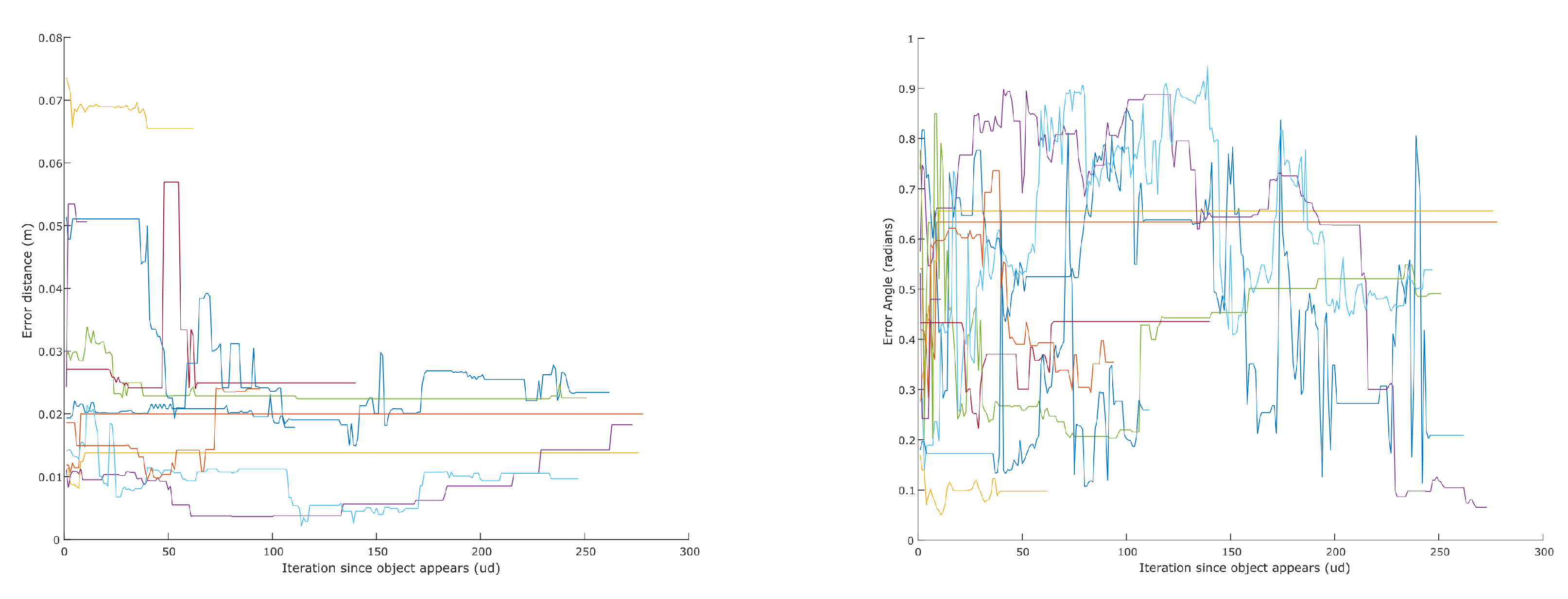
| Error | Mean | σ |
|---|---|---|
| centroid (m) | 0.0256 | 0.1356 |
| angle (rad) | 0.3831 | 0.4320 |
© 2016 by the authors; licensee MDPI, Basel, Switzerland. This article is an open access article distributed under the terms and conditions of the Creative Commons Attribution (CC-BY) license (http://creativecommons.org/licenses/by/4.0/).
Share and Cite
Ramon Soria, P.; Bevec, R.; Arrue, B.C.; Ude, A.; Ollero, A. Extracting Objects for Aerial Manipulation on UAVs Using Low Cost Stereo Sensors. Sensors 2016, 16, 700. https://0-doi-org.brum.beds.ac.uk/10.3390/s16050700
Ramon Soria P, Bevec R, Arrue BC, Ude A, Ollero A. Extracting Objects for Aerial Manipulation on UAVs Using Low Cost Stereo Sensors. Sensors. 2016; 16(5):700. https://0-doi-org.brum.beds.ac.uk/10.3390/s16050700
Chicago/Turabian StyleRamon Soria, Pablo, Robert Bevec, Begoña C. Arrue, Aleš Ude, and Aníbal Ollero. 2016. "Extracting Objects for Aerial Manipulation on UAVs Using Low Cost Stereo Sensors" Sensors 16, no. 5: 700. https://0-doi-org.brum.beds.ac.uk/10.3390/s16050700