Customizable Optical Force Sensor for Fast Prototyping and Cost-Effective Applications


 , , and
Abstract
:1. Introduction
1.1. Background
- Feedback in an impedance control system,
- Comparison with a threshold to limit the interaction force between user and device for safety reasons,
- Detection of movement intention,
- Measurements to develop objective clinical assessment systems.
1.2. State of the Art
- In case of torque sensors, they measure the load in the motor shaft, which in over-constrained mechanisms implies not measuring all the interaction forces. Additionally, they are limited to be used with rotary actuators.
- The main shortcoming of strain gauges is the difficulty in their placement and fixation. Strain gauges must be glued firmly to a surface that deforms in a concrete way, resulting in relatively complex geometries or miniaturization hardly achievable without specialized material assets.
- There is a wide variety of miniature load cells; however, most of them can only measure compression forces, while compression–extension sensors may result unaffordable or not sufficiently miniaturized.
- Force-sensing resistors depend heavily on the surface contact and are not sufficiently reliable to be considered for this application.
- Other technologies like Hall effect force sensors may result in high-consumption and bulky solutions that can be integrated only in the biggest wearable devices.
1.3. Objectives
2. Materials and Methods
2.1. Hardware Description
2.1.1. Optical Architecture
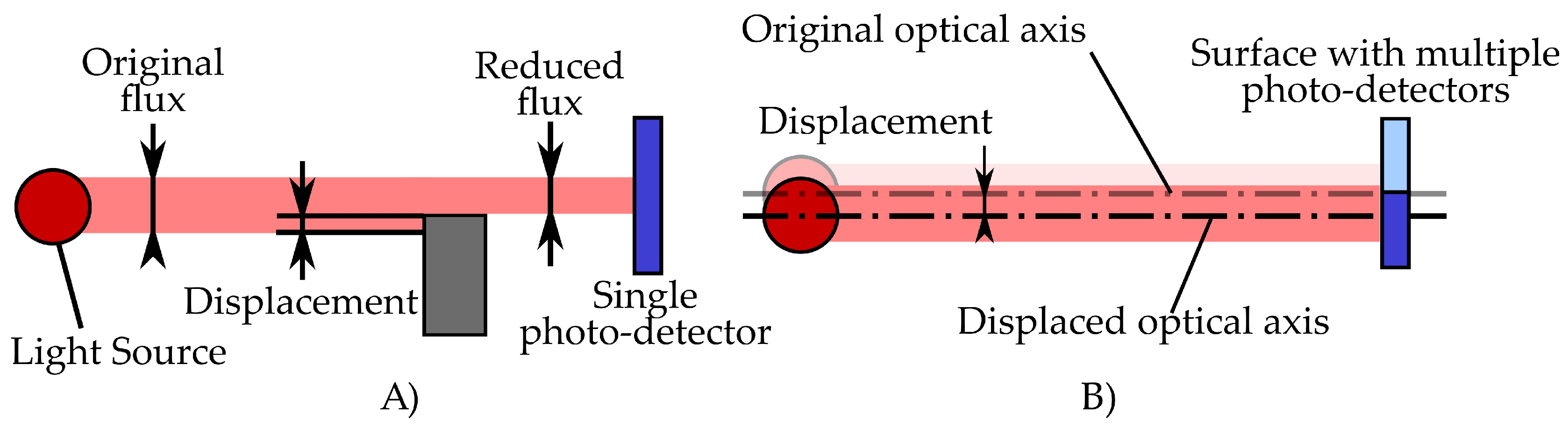
- A point light source, which emits a directionless light front.
- A pinhole to narrow the light front, reducing the stray light and obtaining the light beam.
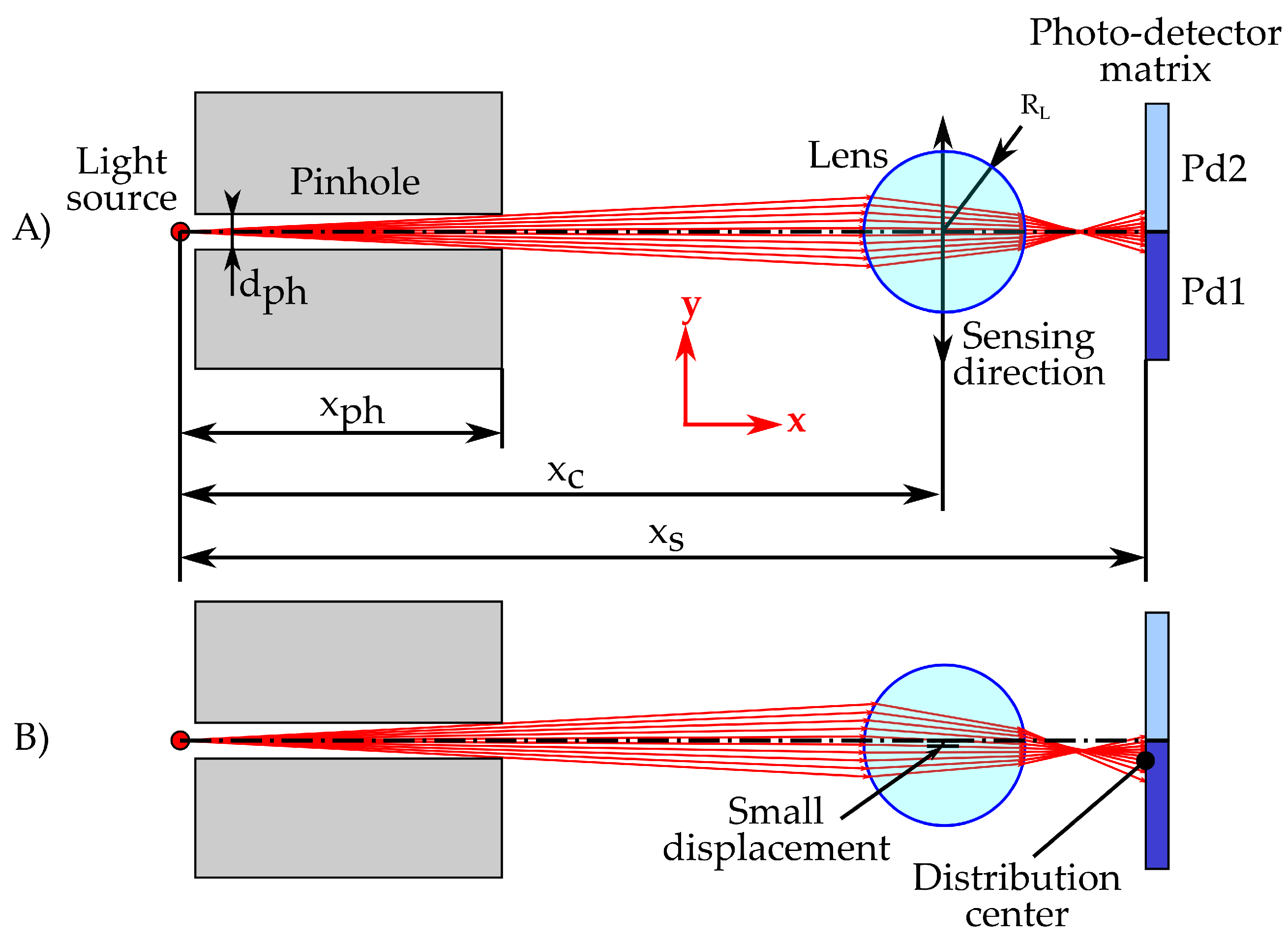
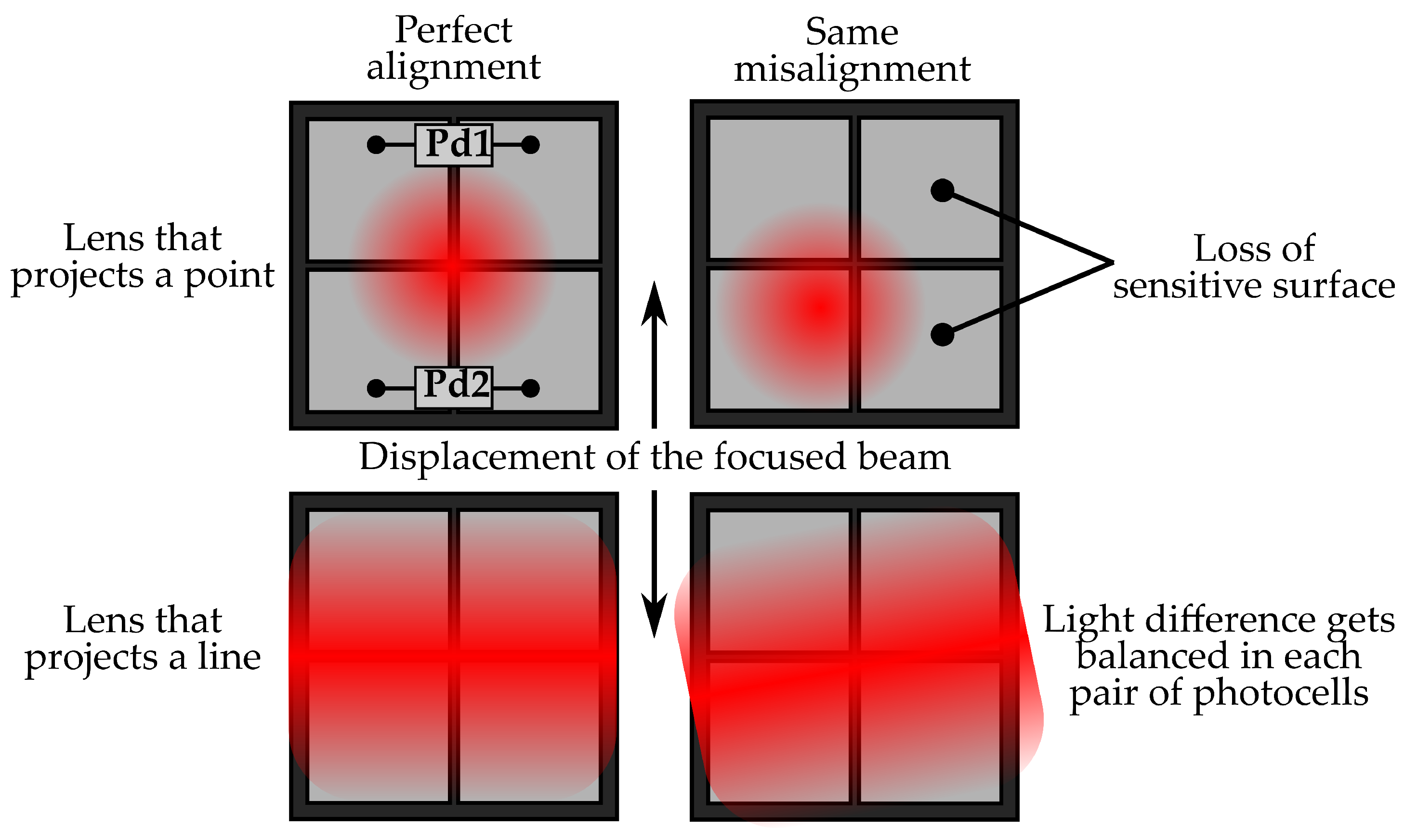
- A lens that refracts the light beam and collimates it over the light sensitive surface. This element will be the element subdued to the displacement to be measured. It will have a focal length short enough to induce a high deviation of the light beam when a small misalignment is applied (Figure 2, Bottom).
- A light sensing surface, composed of a matrix of photo-detectors so the position in which the light is focused can be determined by the difference of the light measured in each element of the matrix.
- Once generated, the first intersection (,) between each ray and the spherical lens is computed solving the Equations (4) and (5). In each intersection, the normal vector to the surface () and a vector () with the same direction than the incident ray and modulus equal to the refractive index () of the propagation medium are computed using Equations (6) and (7):
- Steps 2 and 3 solve the refraction of a light beam (composed by multiple rays) that interacts with an arbitrary surface that separates two mediums with different refractive indexes. This procedure generates a new set of rays, which can be described using the Equations (10) to (12), by their origin (, ) and the angle that defines the direction of propagation (), similarly to the original set:
- Steps 2 to 4 are performed again with the new refracted beam in order to compute the second refraction, which happens when it crosses the interface that separates the lens medium and the air. The resulting set of rays (, , ) corresponds to the beam focused by the lens.
- Finally, the intersection of each resulting ray with the photo-sensitive surface () is determined by Equation (13). The individual photo-detector excited by each ray can be determined by the computed coordinate , so the histogram of the number of rays per each photo-cell can be easily obtained:
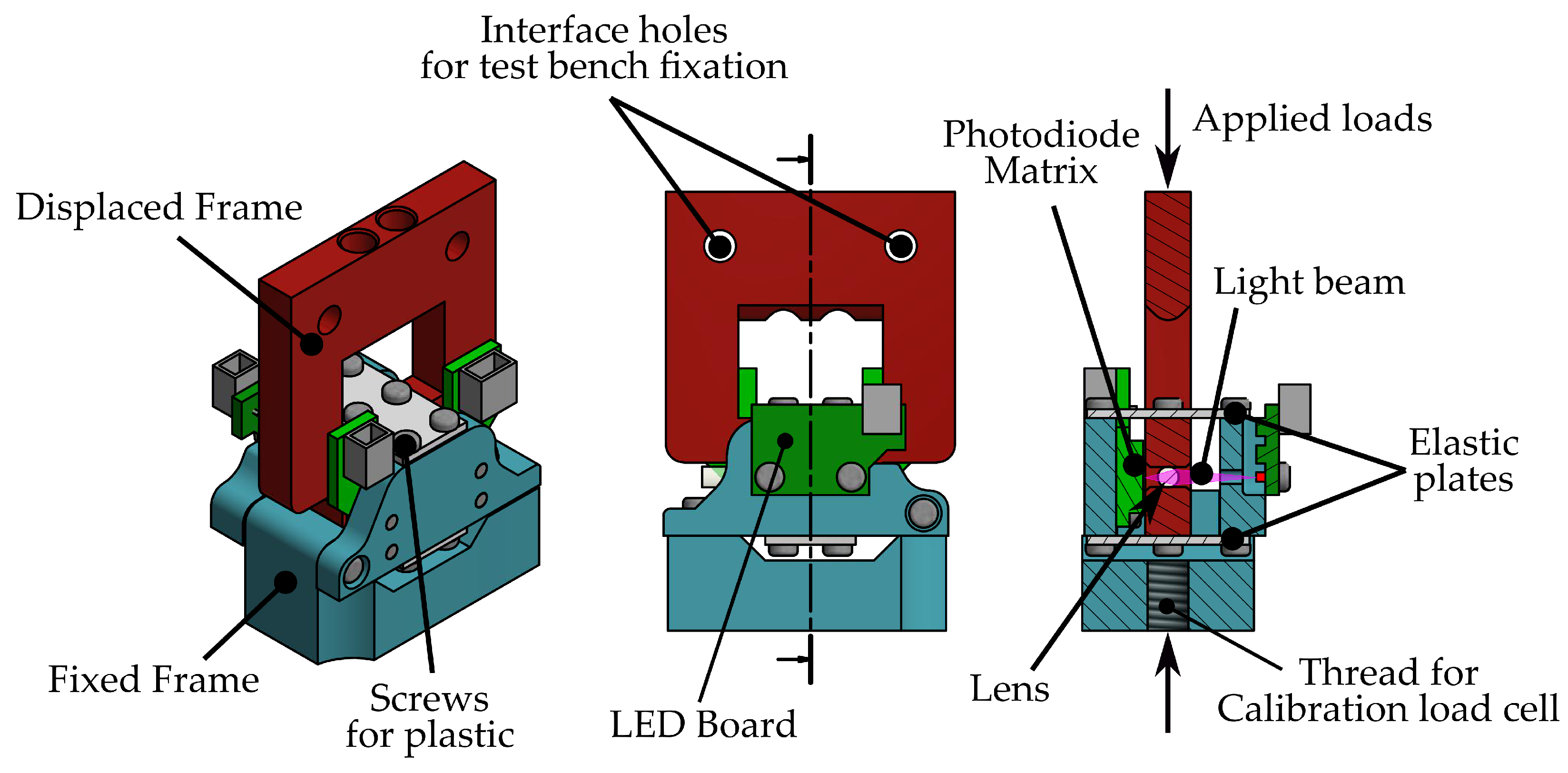
2.1.2. Elastic Frame
2.1.3. Manufacturing Process
2.1.4. Particular Implementation
- Optical assembly
- –
- Light source: LED Kingbright APTD1608LSECK/J3-PF (Taipei, China), Red Color.
- –
- Pinhole data: mm, mm, W
- –
- Lens data: PMMA Cylindrical lens, mm, mm,
- –
- Phodo-detector: OPR5911 Quad Photodiode, 2 × 2 Matrix. Phodo-diode size: 1.27 mm, responsitivity mA/mW, mm.
- Elastic frame
- –
- Effective plate length: mm
- –
- Plate width: mm
- –
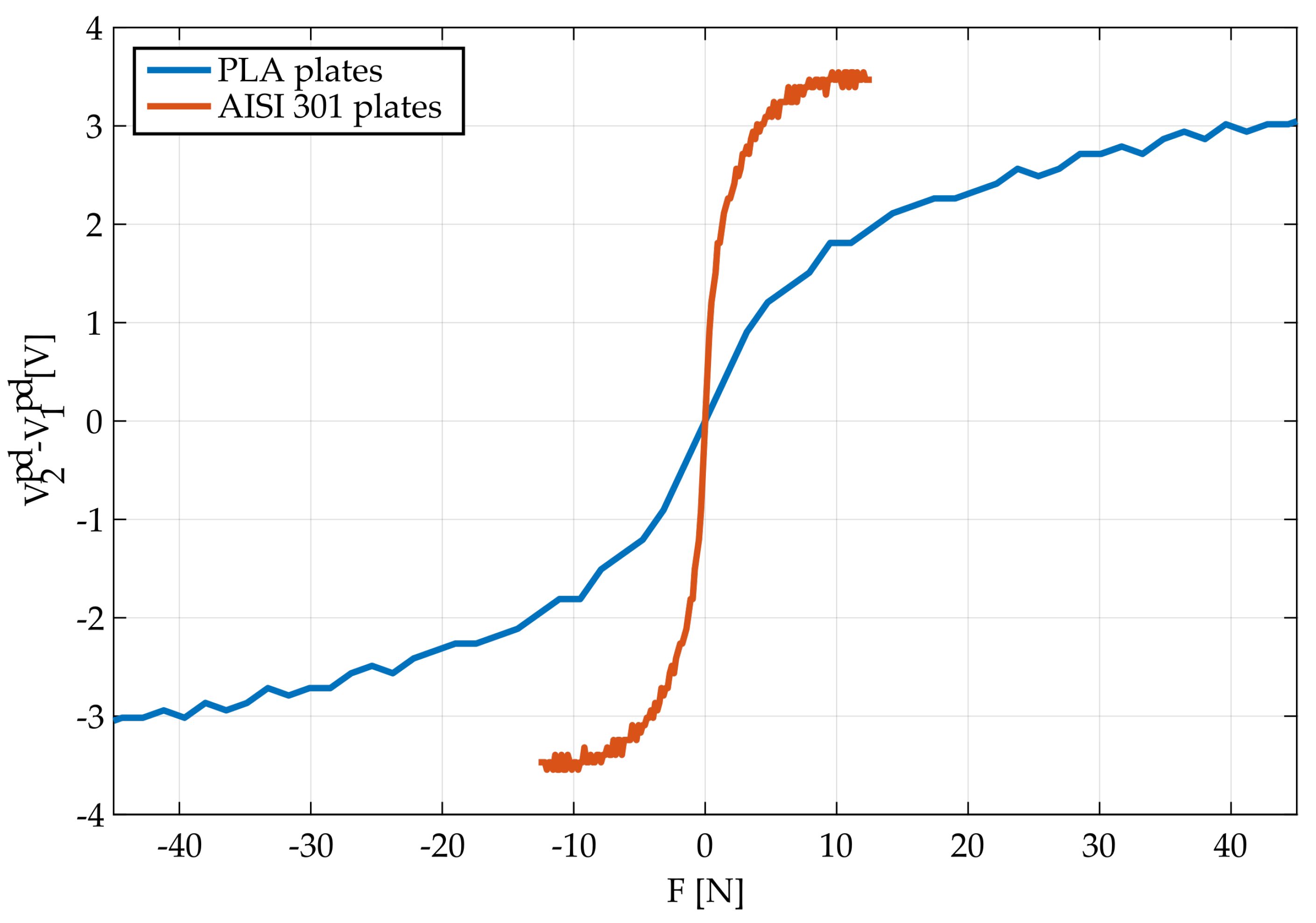
- Plate thickness for PLA case: mm
- –
- Plate thickness for AISI 301 case: mm
- –
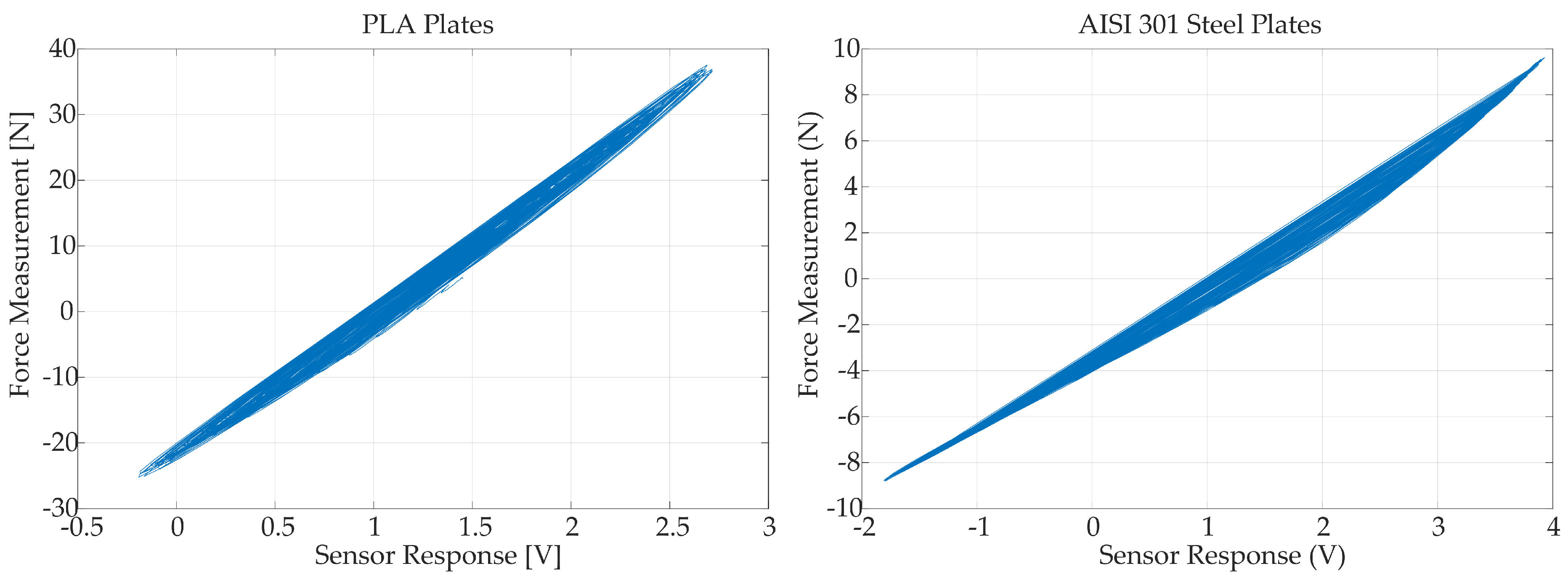
- Expected range of measurement for PLA case: N
- –
- Expected range of measurement for AISI 301 case: N
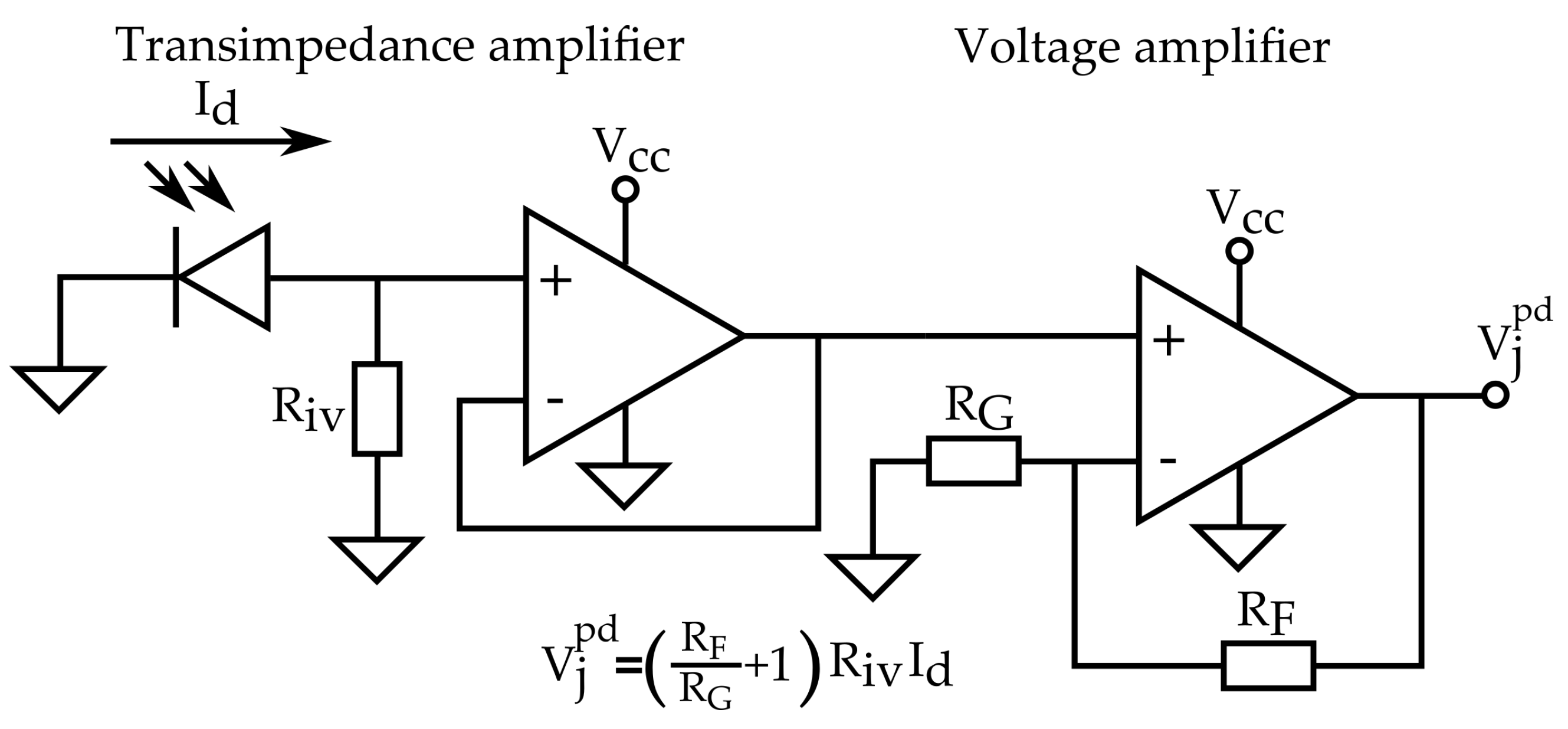
2.2. Signal Conditioning, Acquisition and Processing
- Operational amplifiers: 2× Quadruple general-purpose TI LM324 (One device per pair of photo-diodes).
- Resistance values: k, k, k.
- Resulting conversion factor: V/mA
- Micro-controller: ATmega1280 that features V and 10 bit ADC.
- Digital filter: Mean filter with a time window of eight values.
2.3. Fitting Models
2.3.1. Polynomial Fit
2.3.2. Generalized Prandtl–Ishlinksii Model
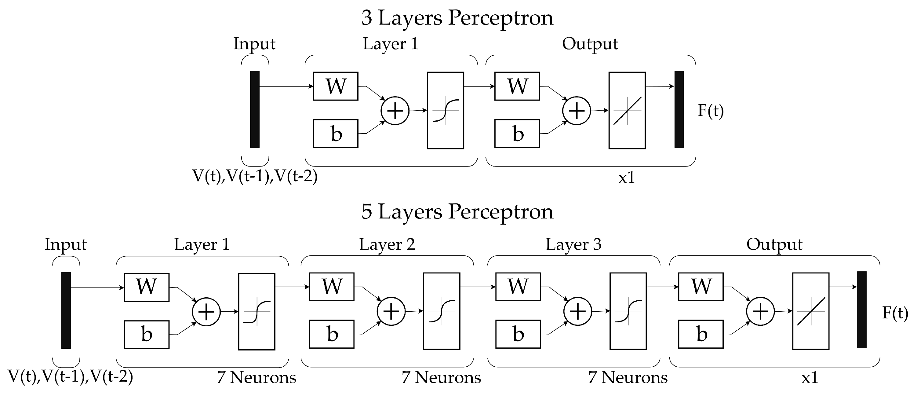
2.3.3. Artificial Neural Networks
- Input layer: three inputs corresponding to , , to be able to model the temporal dependency of the hysteresis.
- Hidden layer: seven neurons with symmetric sigmoid as transfer functions.
- Output layer: one output neuron with linear transfer function that returns the estimated .
- Training algorithm: Levenberg–Marquardt backpropagation algorithm.
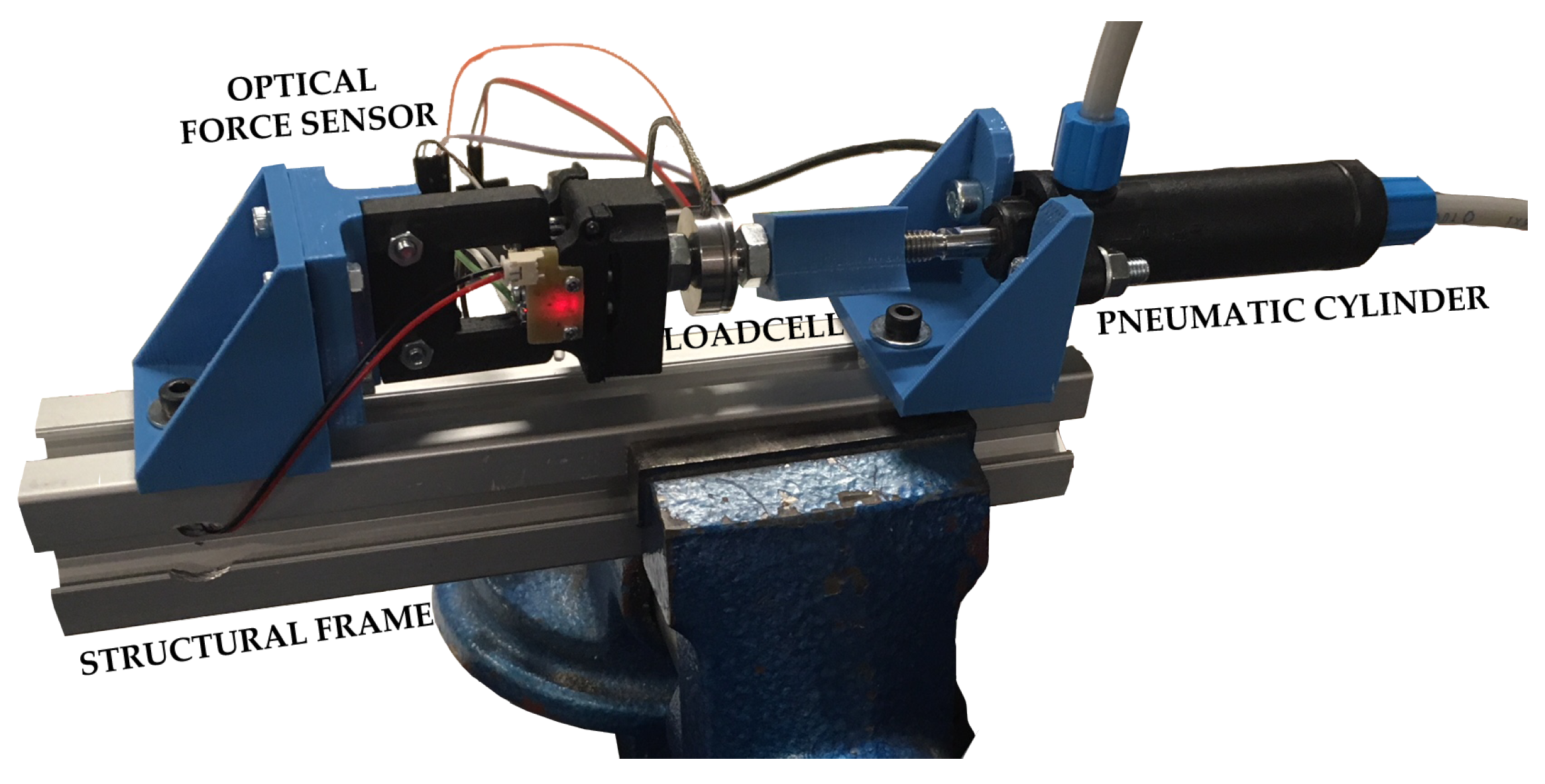
2.4. Experimental Setup
- Optical force sensor. The developed sensor that is going to be validated with the experiment.
- Commercial load cell. A calibrated and industrial grade force sensor, which is used as a reference for the fitting model procedure and validation. The selected load cell model is LCM201–100N manufactured by Omega (Stamford, CT, USA).
- Active element to apply force. A double-acting pneumatic cylinder (Festo DFK-16-40-P (Esslingen, Germany)) is used to apply the desired forces to the force sensors during the experiment. Two proportional pressure control valves (Festo MPPE-3-1/8-10-010) have been selected to control the pressure applied on the cylinder.
- Structural frame. Structure where all elements are mounted.
- 1 Hz sine wave input. Sine signal with a frequency of 1 Hz with the same maximum amplitude (A) previously used in the calibration phase.
- Multi-Frequency wave input. Signal composed of different sine waves in order to obtain a signal with frequency and amplitude variations.
- Random wave input. Signal with random values with a maximum frequency of 1.5 Hz and the maximum amplitude used in the calibration phase (A).
- Human interaction. Signal obtained by direct interaction with the test bench without using the pneumatic cylinder.
3. Results and Discussion
3.1. Real Sensor Performance
3.2. Model Fitting Performance
3.2.1. Polynomial Fit Analysis
3.2.2. Generalized Prandtl–Ishlinskii Model Analysis
3.2.3. Multilayer Perceptron Analysis
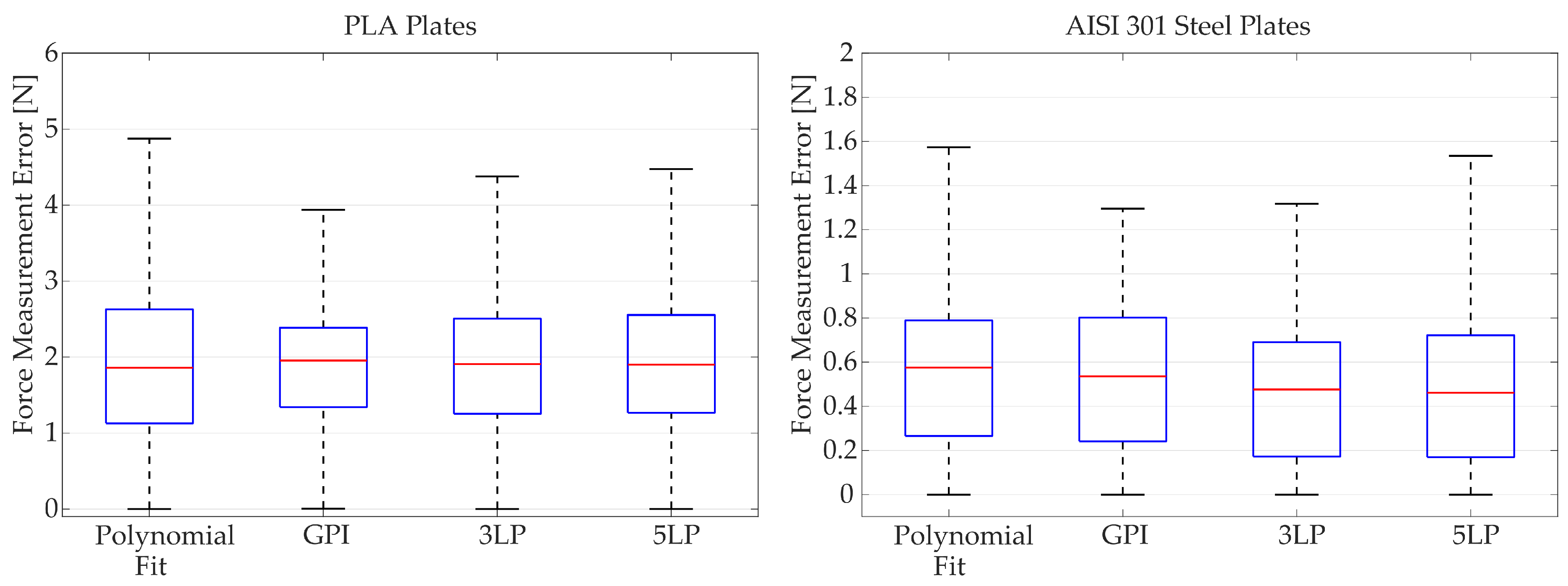
3.2.4. Comparative Analysis
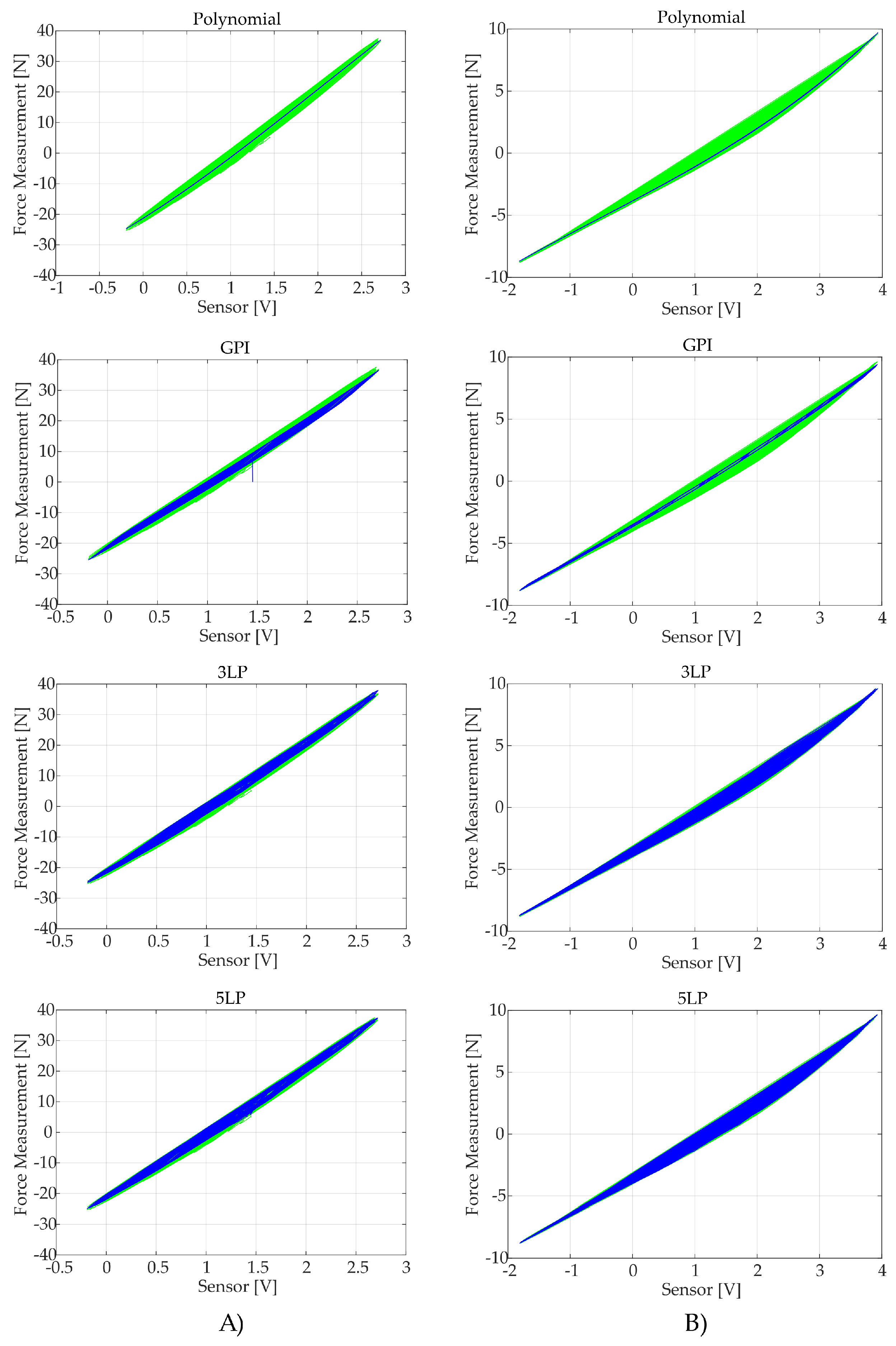
- Polynomial fit: It is the most simple model, which does not need a complex infrastructure to be calibrated. It normally achieves a centered solution that, despite not correcting the hysteresis, can distribute the error across all measurement ranges. Additionally, due to the simplicity of the required mathematical operations, this is the fastest model to evaluate, which allows its implementation in real-time applications without requiring much computing power. This approximation may be the suitable for applications where only the dynamic evolution of the force is interesting, such as movement intention detection, endstops or coarse force controllers.
- Generalized Prandtl–Ishlinskii model: This is the most balanced model, which has enough free parameters to be able to model an hysteresis cycle while avoiding overfitting artifacts. It must be pointed out that, due to limitations of the optimization process, this alternative was trained with only the 2.5% of the acquired calibration data. Therefore, one can conclude that this model is outstanding concerning the generalization capability, being able to successfully extrapolate non-trained inputs. Its main disadvantage is the computational cost that requires its optimization. Additionally, when evaluating individual samples, it is almost 350 times slower (RCT) than the polynomial counterpart, which does not imply that it cannot be implemented for real-time applications, but it will require more computing power for the same sampling frequency. With well-chosen envelope functions, this might be the most suitable model for applications where the applied force pattern is unforeseeable, such as accurate measurements of human–machine interaction.
- Multilayer Perceptrons: Perceptrons are halfway solutions between polynomials and GPI. Like most artificial neural networks, they suffer from lack of generalization capability, so they can lead to wrong extrapolation or overfitting and attention must be paid when choosing their architecture. However, they are easy to train, require moderate computing power, and provide outstanding results when the working conditions are similar to the training ones.
4. Conclusions
Acknowledgments
Author Contributions
Conflicts of Interest
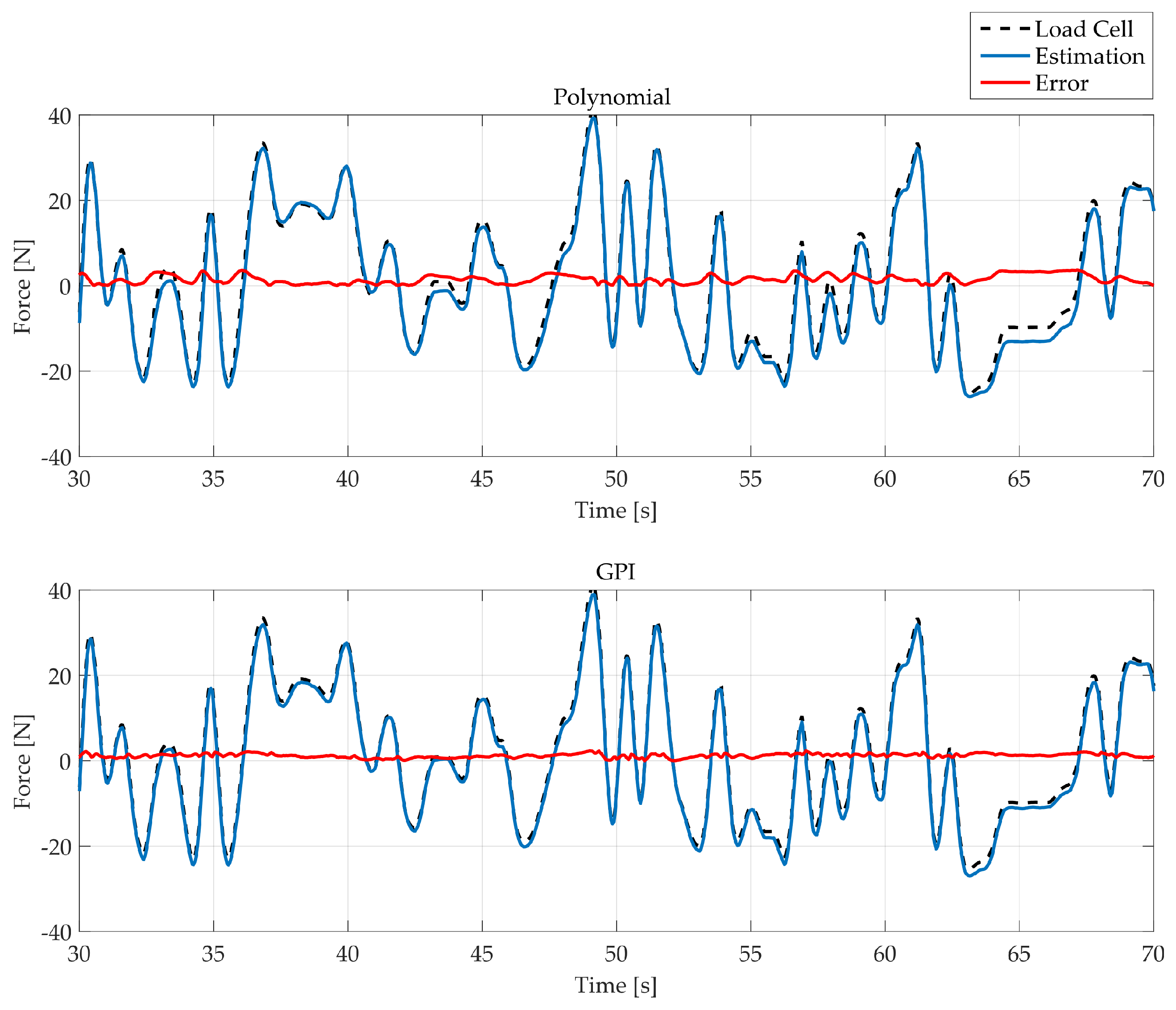
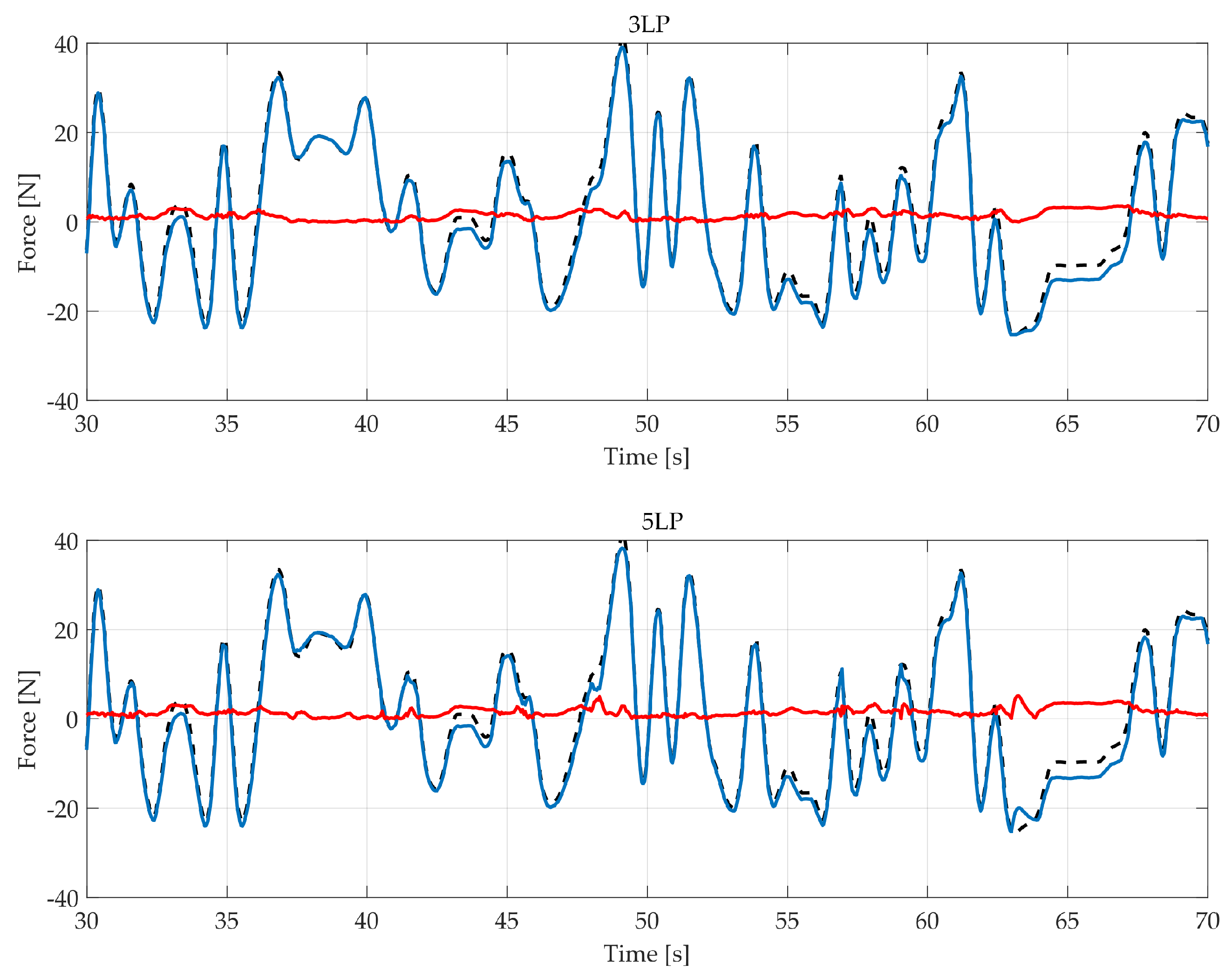
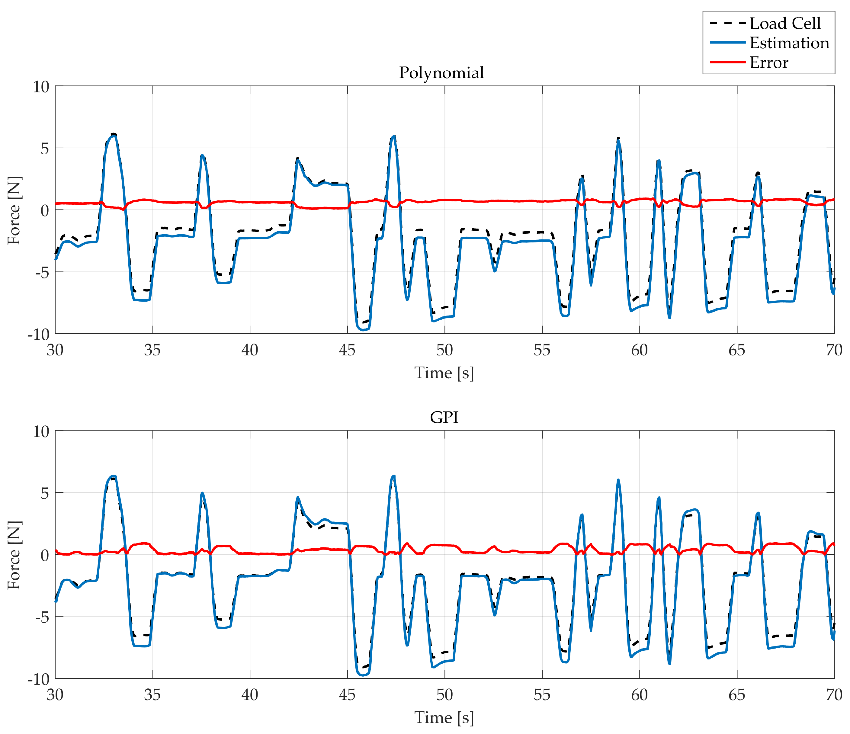
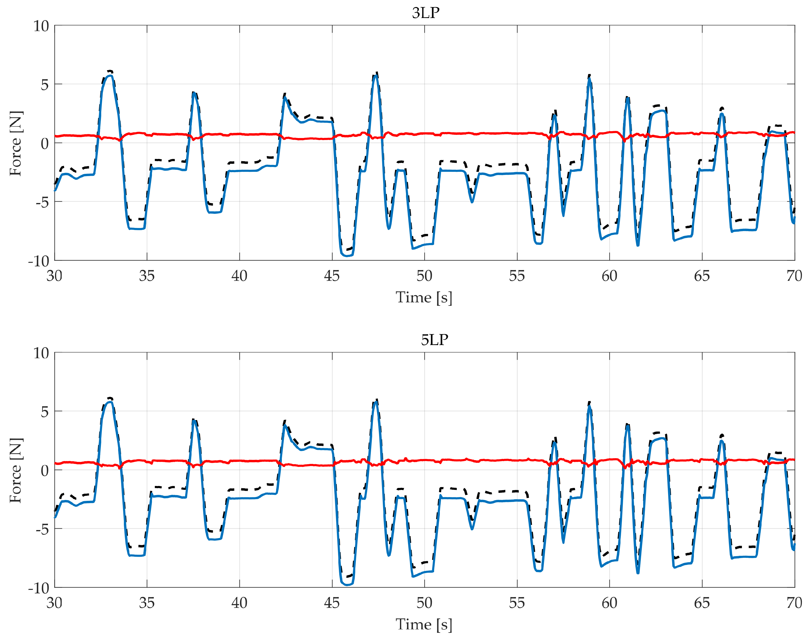
Appendix A. Experimental Validation: Detailed Figures
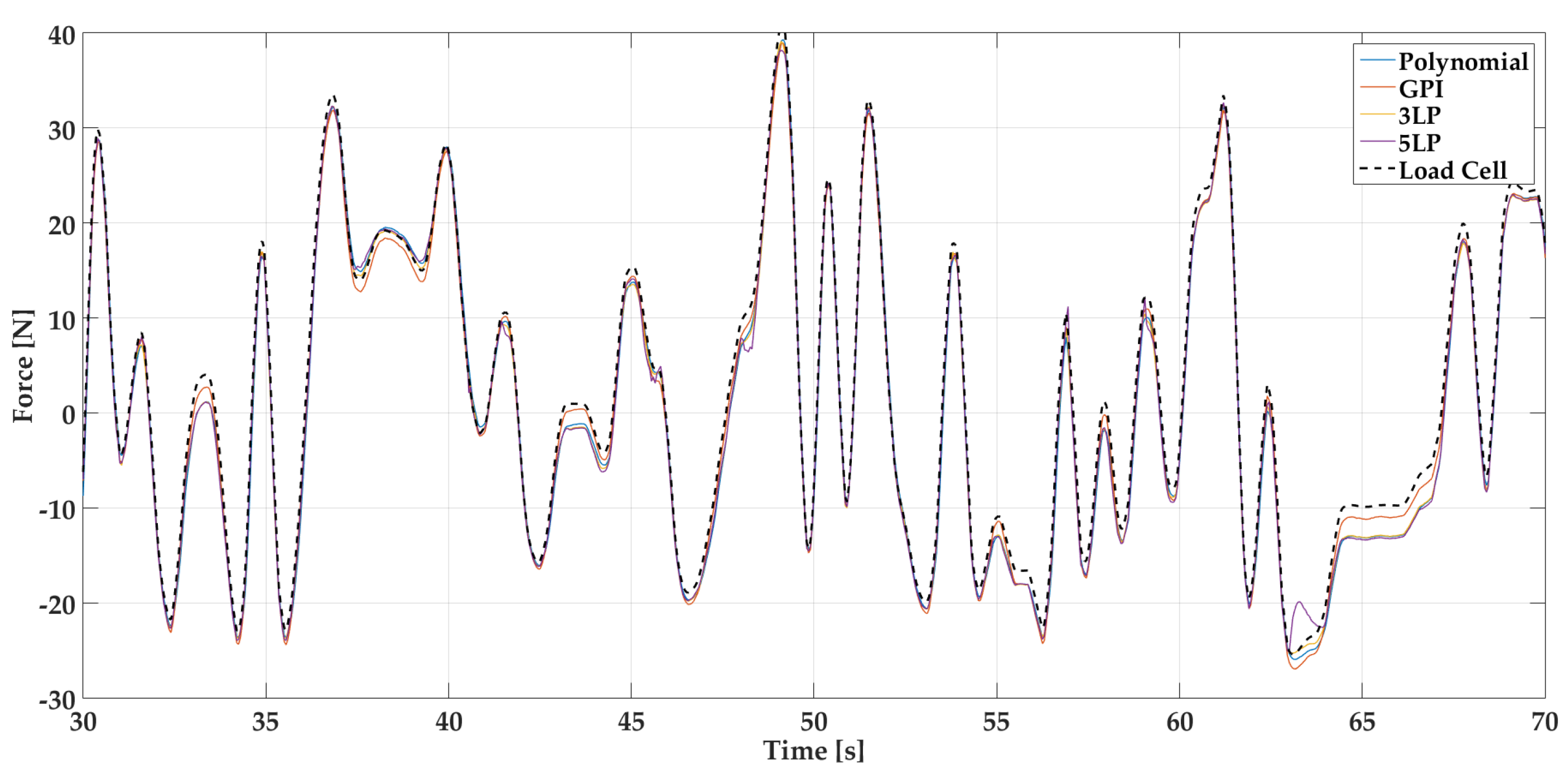
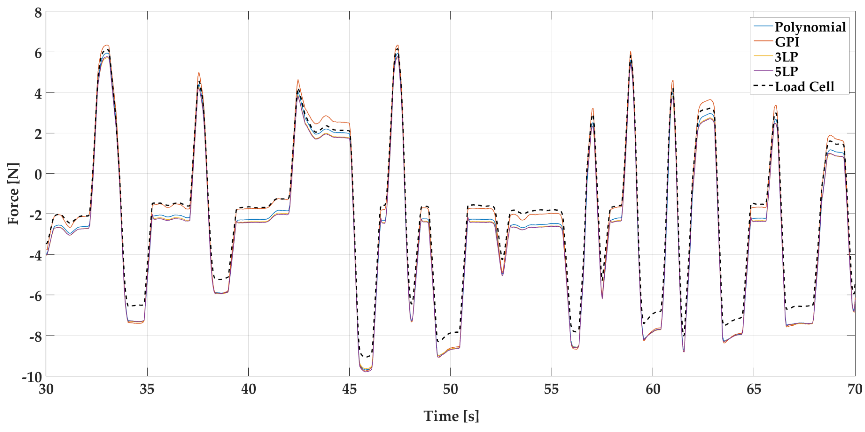
Appendix A.1. Comparison of the Response of the Computed Fitting Models

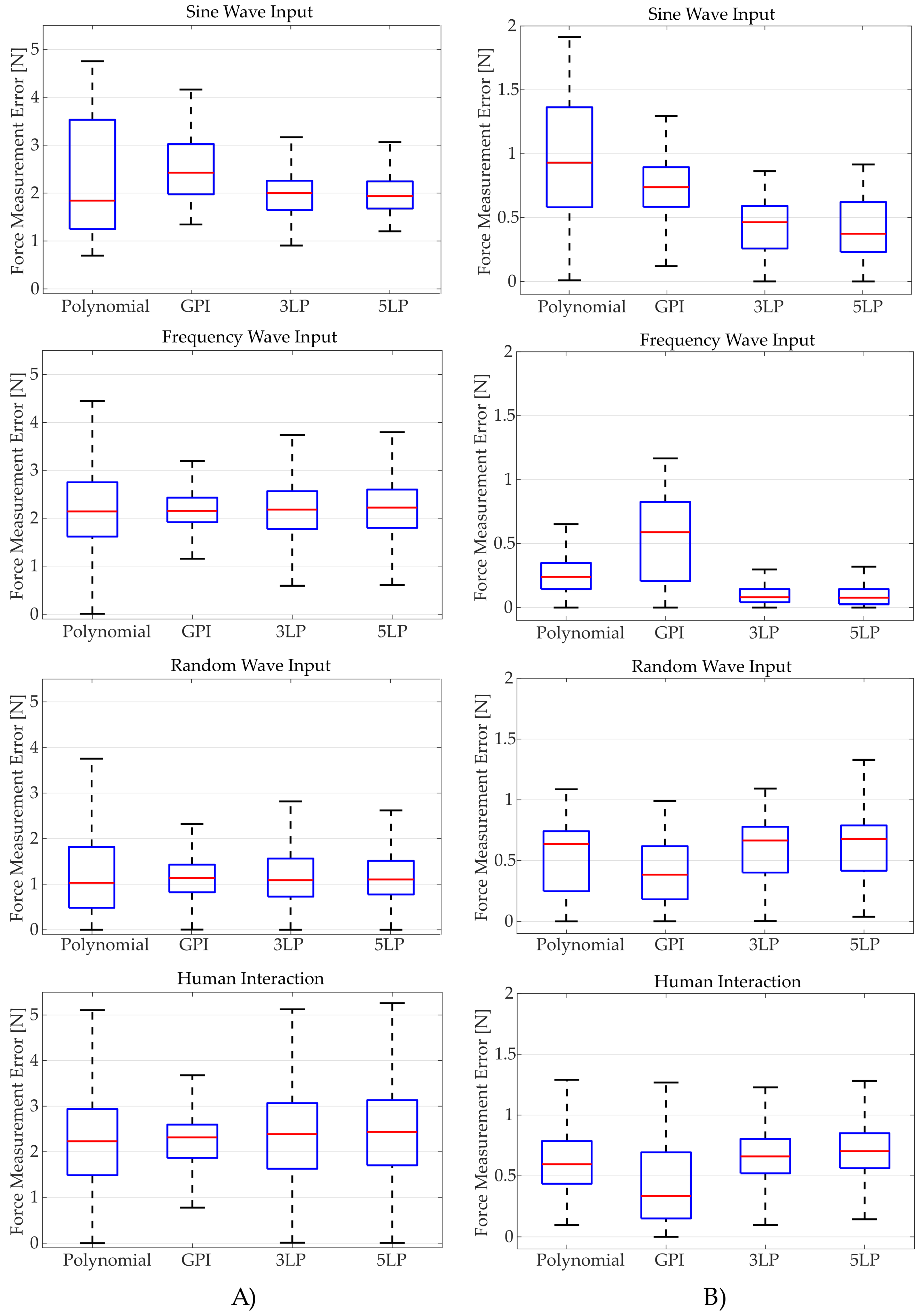
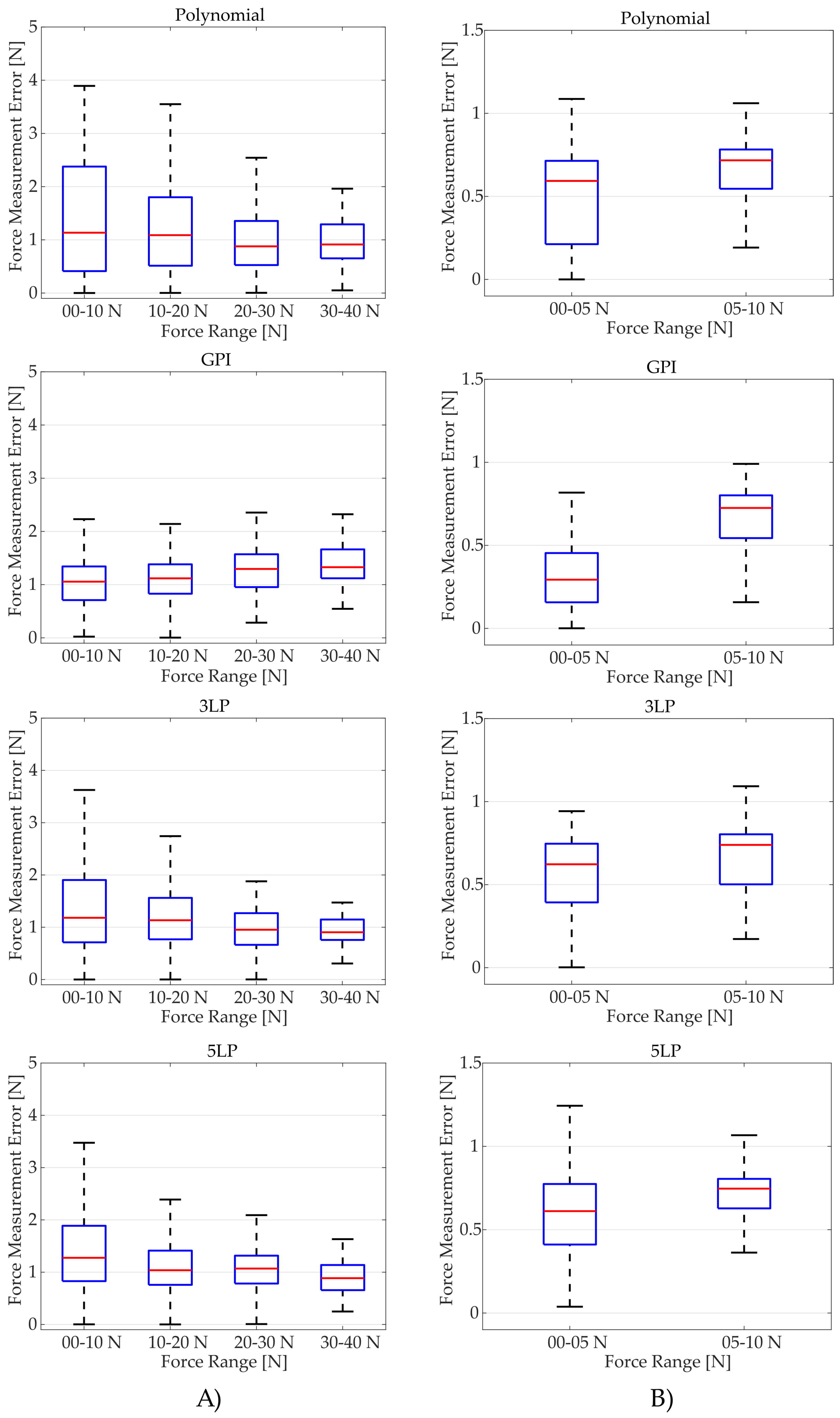
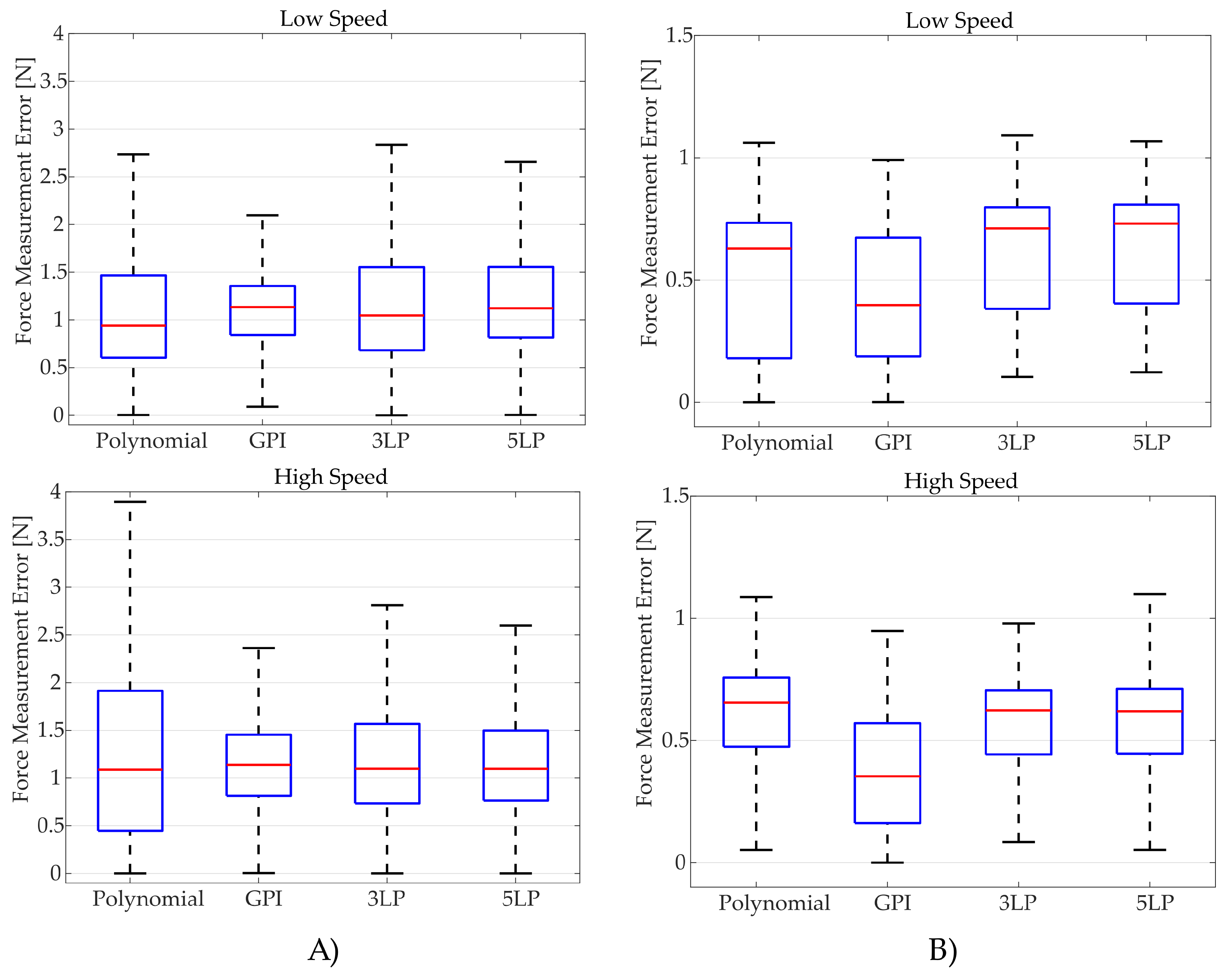
Appendix A.2. Error Distributions of the Fitted Models


Appendix A.3. Error of Computed Sensor Models with a Human Interaction Input Signal


References
- AIDE: Adaptive Multimodal Interfaces to Assist Disabled People in Daily Activities (GA 645322). Available online: http://cordis.europa.eu/project/rcn/194307_en.html (accessed on 10 January 2018).
- Diez, J.A.; Blanco, A.; Catalan, J.M.; Bertomeu-Motos, A.; Badesa, F.J.; Garcia-Aracil, N. Mechanical Design of a Novel Hand Exoskeleton Driven by Linear Actuators. In Advances in Intelligent Systems and Computing, Proceedings of the ROBOT 2017: Third Iberian Robotics Conference, Seville, Spain, 22–24 November 2017; Ollero, A., Sanfeliu, A., Montano, L., Lau, N., Cardeira, C., Eds.; Springer: Cham, Switzerland, 2018; Volume 694. [Google Scholar]
- Díez, J.A.; Catalán, J.M.; Lledó, L.D.; Badesa, F.J.; Garcia-Aracil, N. Multimodal robotic system for upper-limb rehabilitation in physical environment. Adv. Mech. Eng. 2016, 8, 1–8. [Google Scholar] [CrossRef]
- Schabowsky, C.N.; Godfrey, S.B.; Holley, R.J.; Lum, P.S. Development and pilot testing of HEXORR: Hand EXOskeleton rehabilitation robot. J. NeuroEng. Rehabil. 2010, 7, 36. [Google Scholar] [CrossRef] [PubMed]
- Hyun, D.J. On the Dynamics and Control of a MedicalExoskeleton. Ph.D. Thesis, UC Berkeley, Berkeley, CA, USA, 2012. [Google Scholar]
- Shields, B.L.; Main, J.A.; Peterson, S.W.; Strauss, A.M. An anthropomorphic hand exoskeleton to prevent astronaut hand fatigue during extravehicular activities. IEEE Trans. Syst. Man Cybern. Part A Syst. Hum. 1997, 27, 668–673. [Google Scholar] [CrossRef]
- Yahud, S.; Dokos, S.; Morley, J.W.; Lovell, N.H. Experimental validation of a tactile sensor model for a robotic hand. In Proceedings of the Annual International Conference of the IEEE on Engineering in Medicine and Biology Society (EMBC 2009), Minneapolis, MN, USA, 3–6 September 2009; pp. 2300–2303. [Google Scholar]
- Carrozza, M.C.; Massa, B.; Micera, S.; Lazzarini, R.; Zecca, M.; Dario, P. The development of a novel prosthetic hand-ongoing research and preliminary results. IEEE/ASME Trans. Mechatron. 2002, 7, 108–114. [Google Scholar] [CrossRef]
- Fontana, M.; Marcheschi, S.; Salsedo, F.; Bergamasco, M. A Three-Axis Force Sensor for Dual Finger Haptic Interfaces. Sensors 2012, 12, 13598–13616. [Google Scholar] [CrossRef] [PubMed] [Green Version]
- Fontana, M.; Fabio, S.; Marcheschi, S.; Bergamasco, M. Haptic hand exoskeleton for precision grasp simulation. J. Mech. Robot. 2013, 5, 1–9. [Google Scholar] [CrossRef] [Green Version]
- Chiri, A.; Vitiello, N.; Giovacchini, F.; Roccella, S.; Vecchi, F.; Carrozza, M.C. Mechatronic design and characterization of the index finger module of a hand exoskeleton for post-stroke rehabilitation. IEEE/ASME Trans. Mechatron. 2012, 17, 884–894. [Google Scholar] [CrossRef]
- Rodriguez-Cheu, L.E.; Gonzalez, D.; Rodriguez, M. Result of a perceptual feedback of the grasping forces to prosthetic hand users. In Proceedings of the 2nd IEEE RAS & EMBS International Conference on Biomedical Robotics and Biomechatronics (BioRob 2008), Scottsdale, AZ, USA, 19–22 October 2008; pp. 901–906. [Google Scholar]
- Baker, M.D.; McDonough, M.K.; McMullin, E.M.; Swift, M.; BuSha, B.F. Orthotic hand-assistive exoskeleton. In Proceedings of the 2011 IEEE 37th Annual Northeast Bioengineering Conference (NEBEC), Troy, NY, USA, 1–3 April 2011; pp. 1–2. [Google Scholar]
- Wege, A.; Hommel, G. Development and control of a hand exoskeleton for rehabilitation of hand injuries. In Proceedings of the 2005 IEEE/RSJ International Conference on Intelligent Robots and Systems (IROS 2005), Edmonton, AB, Canada, 2–6 August 2005; pp. 3046–3051. [Google Scholar]
- Johnston, D.; Zhang, P.; Hollerbach, J.; Jacobsen, S. A full tactile sensing suite for dextrous robot hands and use in contact force control. In Proceedings of the 1996 IEEE International Conference on Robotics and Automation, Minneapolis, MN, USA, 22–28 April 1996; Volume 4, pp. 3222–3227. [Google Scholar]
- Pons, J.L.; Rocon, E.; Ceres, R.; Reynaerts, D.; Saro, B.; Levin, S.; Van Moorleghem, W. The MANUS-HAND dextrous robotics upper limb prosthesis: Mechanical and manipulation aspects. Auton. Robot. 2004, 16, 143–163. [Google Scholar] [CrossRef]
- Su, H.; Zervas, M.; Furlong, C.; Fischer, G.S. A miniature MRI-compatible fiber-optic force sensor utilizing fabry-perot interferometer. In MEMS and Nanotechnology; Springer: New York, NY, USA, 2011; Volume 4, pp. 131–136. [Google Scholar]
- Xiao, L.; Yang, T.; Huo, B.; Zhao, X.; Han, J.; Xu, W. Impedance control of a robot needle with a fiber optic force sensor. In Proceedings of the IEEE 13th International Conference on Signal Processing (ICSP), Chengdu, China, 6–10 November 2016; pp. 1379–1383. [Google Scholar]
- Fernandez, A.F.; Berghmans, F.; Brichard, B.; Mégret, P.; Decréton, M.; Blondel, M.; Delchambre, A. Multi-component force sensor based on multiplexed fibre Bragg grating strain sensors. Meas. Sci. Technol. 2001, 12, 810. [Google Scholar] [CrossRef]
- Park, Y.L.; Ryu, S.C.; Black, R.J.; Chau, K.K.; Moslehi, B.; Cutkosky, M.R. Exoskeletal force-sensing end-effectors with embedded optical fiber-Bragg-grating sensors. IEEE Trans. Robot. 2009, 25, 1319–1331. [Google Scholar] [CrossRef]
- Su, H.; Fischer, G.S. A 3-axis optical force/torque sensor for prostate needle placement in magnetic resonance imaging environments. In Proceedings of the IEEE International Conference on Technologies for Practical Robot Applications (TePRA 2009), Woburn, MA, USA, 9–10 November 2009; pp. 5–9. [Google Scholar]
- Hara, M.; Matthey, G.; Yamamoto, A.; Chapuis, D.; Gassert, R.; Bleuler, H.; Higuchi, T. Development of a 2-DOF electrostatic haptic joystick for MRI/fMRI applications. In Proceedings of the IEEE International Conference on Robotics and Automation (ICRA’09), Kobe, Japan, 12–17 May 2009; pp. 1479–1484. [Google Scholar]
- Hirose, S.; Yoneda, K. Development of optical six-axial force sensor and its signal calibration considering nonlinear interference. In Proceedings of the 1990 IEEE International Conference on Robotics and Automation, Cincinnati, OH, USA, 13–18 May 1990; pp. 46–53. [Google Scholar]
- Jeong, S.H.; Lee, H.J.; Kim, K.R.; Kim, K.S. Design of a miniature force sensor based on photointerrupter for robotic hand. Sens. Actuators A Phys. 2018, 269, 444–453. [Google Scholar] [CrossRef]
- Palli, G.; Hosseini, M.; Melchiorri, C. A simple and easy-to-build optoelectronics force sensor based on light fork: Design comparison and experimental evaluation. Sens. Actuators A Phys. 2018, 269, 369–381. [Google Scholar] [CrossRef]
- Takahashi, N.; Tada, M.; Ueda, J.; Matsumoto, Y.; Ogasawara, T. An optical 6-axis force sensor for brain function analysis using fMRI. In Proceedings of the IEEE on Sensors, Toronto, ON, Canada, 22–24 October 2003; Volume 1, pp. 253–258. [Google Scholar]
- Tada, M.; Kanade, T. An MR-compatible optical force sensor for human function modeling. In Medical Image Computing and Computer-Assisted Intervention–MICCAI 2004; Springer: Berlin/Heidelberg, Germany, 2004; pp. 129–136. [Google Scholar]
- Tada, M.; Kanade, T. Design of an MR-compatible three-axis force sensor. In Proceedings of the 2005 IEEE/RSJ International Conference on Intelligent Robots and Systems (IROS 2005), Edmonton, AB, Canada, 2–6 August 2005; pp. 3505–3510. [Google Scholar]
- Glassner, A.S. (Ed.) An Introduction to Ray Tracing; Elsevier: Amsterdam, The Netherlands, 1989. [Google Scholar]
- Lanzotti, A.; Grasso, M.; Staiano, G.; Martorelli, M. The impact of process parameters on mechanical properties of parts fabricated in PLA with an open-source 3-D printer. Rapid Prototyp. J. 2015, 21, 604–617. [Google Scholar] [CrossRef]
- Díez, J.A.; Blanco, A.; Catalán, J.M.; Badesa, F.J.; Lledó, L.D.; Garcia-Aracil, N. Hand exoskeleton for rehabilitation therapies with integrated optical force sensor. Adv. Mech. Eng. 2018, 10, 1–11. [Google Scholar] [CrossRef]
- Al Janaideh, M.; Rakheja, S.; Su, C.Y. An analytical generalized Prandtl–Ishlinskii model inversion for hysteresis compensation in micropositioning control. IEEE/ASME Trans. Mechatron. 2011, 16, 734–744. [Google Scholar] [CrossRef]
- Sayyaadi, H.; Zakerzadeh, M.R.; Zanjani, M.A.V. Accuracy evaluation of generalized Prandtl-Ishlinskii model in characterizing asymmetric saturated hysteresis nonlinearity behavior of shape memory alloy actuators. Int. J. Res. Rev. Mechatron. Des. Simul. 2011, 1, 59–68. [Google Scholar]
- Zhang, J.; Merced, E.; Sepúlveda, N.; Tan, X. Modeling and inverse compensation of hysteresis in vanadium dioxide using an extended generalized Prandtl–Ishlinskii model. Smart Mater. Struct. 2014, 23, 125017. [Google Scholar] [CrossRef]
- Sánchez-Durán, J.A.; Oballe-Peinado, Ó.; Castellanos-Ramos, J.; Vidal-Verdú, F. Hysteresis correction of tactile sensor response with a generalized Prandtl–Ishlinskii model. Microsyst. Technol. 2012, 18, 1127–1138. [Google Scholar] [CrossRef]
- Liu, S.; Su, C.Y.; Li, Z. Robust adaptive inverse control of a class of nonlinear systems with Prandtl-Ishlinskii hysteresis model. IEEE Trans. Autom. Control 2014, 59, 2170–2175. [Google Scholar] [CrossRef]
- Maren, A.J.; Harston, C.T.; Pap, R.M. Handbook of Neural Computing Applications; Academic Press: Cambridge, MA, USA, 2014. [Google Scholar]
- Islam, T.; Saha, H. Hysteresis compensation of a porous silicon relative humidity sensor using ANN technique. Sens. Actuators B Chem. 2006, 114, 334–343. [Google Scholar] [CrossRef]
- Lin, F.J.; Shieh, H.J.; Huang, P.K. Adaptive wavelet neural network control with hysteresis estimation for piezo-positioning mechanism. IEEE Trans. Neural Netw. 2006, 17, 432–444. [Google Scholar] [CrossRef] [PubMed]
- Wang, H.; Song, G. Innovative NARX recurrent neural network model for ultra-thin shape memory alloy wire. Neurocomputing 2014, 134, 289–295. [Google Scholar] [CrossRef]
- Zhou, M.; Wang, Y.; Xu, R.; Zhang, Q.; Zhu, D. Feed-forward control for magnetic shape memory alloy actuators based on the radial basis function neural network model. J. Appl. Biomater. Funct. Mater. 2017, 15, 25–30. [Google Scholar] [CrossRef] [PubMed]
- Murtagh, F. Multilayer perceptrons for classification and regression. Neurocomputing 1991, 2, 183–197. [Google Scholar] [CrossRef]
- Irie, B.; Miyake, S. Capabilities of three-layered perceptrons. In Proceedings of the IEEE International Conference on Neural Networks, San Diego, CA, USA, 24–27 July 1988; Volume 1, p. 218. [Google Scholar]
- Yang, M.J.; Gu, G.Y.; Zhu, L.M. Parameter identification of the generalized Prandtl–Ishlinskii model for piezoelectric actuators using modified particle swarm optimization. Sens. Actuators A Phys. 2013, 189, 254–265. [Google Scholar] [CrossRef]


| Input | Variable | Polynomial Fit | GPI Model | 3LP | 5LP | ||||
|---|---|---|---|---|---|---|---|---|---|
| PLA | STEEL | PLA | STEEL | PLA | STEEL | PLA | STEEL | ||
| Sine Wave | MAE (N) | 2.3147 | 0.9379 | 2.5134 | 0.7312 | 1.9853 | 0.4288 | 1.9974 | 0.4091 |
| MEDIAN (N) | 1.8432 | 0.9299 | 2.4267 | 0.7378 | 1.9999 | 0.4639 | 1.9372 | 0.37341 | |
| SD (N) | 1.2147 | 0.4754 | 0.8571 | 0.2227 | 0.4484 | 0.2059 | 0.4209 | 0.2232 | |
| Corr Coef | 0.9979 | 0.9969 | 0.9991 | 0.9994 | 0.9998 | 0.9997 | 0.9998 | 0.9997 | |
| Outliers (%) | 0.1050 | 0.0253 | 0.1050 | 0.1519 | 0.4202 | 0.0506 | 0.7353 | 0.0253 | |
| Multi-Frequency Wave | MAE (N) | 2.2222 | 0.2916 | 2.1924 | 0.5386 | 2.2024 | 0.1076 | 2.2551 | 0.1033 |
| MEDIAN (N) | 2.1415 | 0.2383 | 2.1531 | 0.5879 | 2.1800 | 0.0790 | 2.2220 | 0.0753 | |
| SD (N) | 0.9141 | 0.2490 | 0.4228 | 0.3327 | 0.6876 | 0.0985 | 0.7718 | 0.1130 | |
| Corr Coef | 0.9972 | 0.9948 | 0.9994 | 0.9927 | 0.9985 | 0.9993 | 0.9970 | 0.9992 | |
| Outliers (%) | 1.1416 | 9.3394 | 2.4099 | 0.0506 | 4.3379 | 5.5176 | 5.7585 | 4.6064 | |
| Random Wave | MAE (N) | 1.2371 | 0.5313 | 1.1349 | 0.4083 | 1.1916 | 0.6022 | 1.2634 | 0.6155 |
| MEDIAN (N) | 1.0303 | 0.6371 | 1.1378 | 0.3845 | 1.0863 | 0.6653 | 1.1042 | 0.6788 | |
| SD (N) | 0.9150 | 0.2740 | 0.4989 | 0.2593 | 0.6863 | 0.2144 | 0.8307 | 0.2179 | |
| Corr Coef | 0.9976 | 0.9992 | 0.9995 | 0.9988 | 0.9990 | 0.9994 | 0.9980 | 0.9995 | |
| Outliers (%) | 0.0761 | 0.0253 | 0.1015 | 0.0253 | 2.8412 | 0.0253 | 6.7986 | 0.0253 | |
| Human Interaction | MAE (N) | 2.2618 | 0.6221 | 2.2643 | 0.4325 | 2.4103 | 0.6754 | 2.4798 | 0.7165 |
| MEDIAN (N) | 2.2304 | 0.5953 | 2.3151 | 0.3345 | 2.3873 | 0.6594 | 2.4370 | 0.7032 | |
| SD (N) | 1.0011 | 0.2475 | 0.7065 | 0.3425 | 0.9520 | 0.2239 | 1.0353 | 0.2043 | |
| Corr Coef | 0.9966 | 0.9991 | 0.9988 | 0.9979 | 0.9973 | 0.9989 | 0.9960 | 0.9995 | |
| Outliers (%) | 0.4225 | 0.0253 | 4.1127 | 0.0253 | 0.1690 | 1.8983 | 0.4225 | 0.2278 | |
| Overall Statistics | RCT | 1.0 | 345.87 | 109.56 | 137.56 | ||||
| MAE (N) | 1.9271 | 0.5958 | 1.9011 | 0.5276 | 1.9236 | 0.4535 | 1.9841 | 0.4611 | |
| MEDIAN (N) | 1.8601 | 0.5753 | 2.0568 | 0.5359 | 2.1305 | 0.4762 | 2.2193 | 0.4608 | |
| SD (N) | 1.0751 | 0.3995 | 0.7849 | 0.32001 | 0.9160 | 0.2915 | 0.9945 | 0.3048 | |
| Corr Coef | 0.9964 | 0.9956 | 0.9984 | 0.9945 | 0.9977 | 0.9985 | 0.9967 | 0.9985 | |
| Outliers (%) | 0.2341 | 2.4487 | 0.6378 | 0.03164 | 0.7831 | 0.0063 | 1.6712 | 0.0190 | |
© 2018 by the authors. Licensee MDPI, Basel, Switzerland. This article is an open access article distributed under the terms and conditions of the Creative Commons Attribution (CC BY) license (http://creativecommons.org/licenses/by/4.0/).
Share and Cite
Díez, J.A.; Catalán, J.M.; Blanco, A.; García-Perez, J.V.; Badesa, F.J.; Gacía-Aracil, N. Customizable Optical Force Sensor for Fast Prototyping and Cost-Effective Applications. Sensors 2018, 18, 493. https://0-doi-org.brum.beds.ac.uk/10.3390/s18020493
Díez JA, Catalán JM, Blanco A, García-Perez JV, Badesa FJ, Gacía-Aracil N. Customizable Optical Force Sensor for Fast Prototyping and Cost-Effective Applications. Sensors. 2018; 18(2):493. https://0-doi-org.brum.beds.ac.uk/10.3390/s18020493
Chicago/Turabian StyleDíez, Jorge A., José M. Catalán, Andrea Blanco, José V. García-Perez, Francisco J. Badesa, and Nicolás Gacía-Aracil. 2018. "Customizable Optical Force Sensor for Fast Prototyping and Cost-Effective Applications" Sensors 18, no. 2: 493. https://0-doi-org.brum.beds.ac.uk/10.3390/s18020493