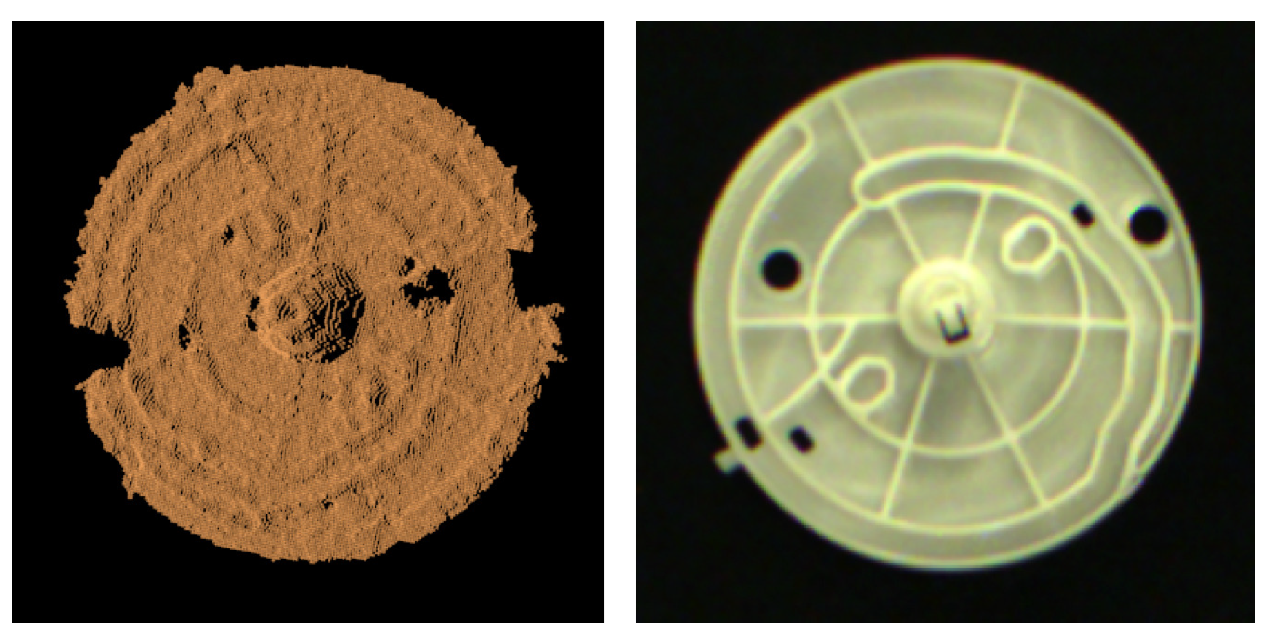
Figure 1.
Defective point cloud of Part A (Left: The captured point cloud of the part; Right: The appearacne of the part). The detailed point cloud of the ridges in the part cannot be captured with the embedded 3D sensor algorithm. Thus, some previous methods fail to estimate the rotation around the center.
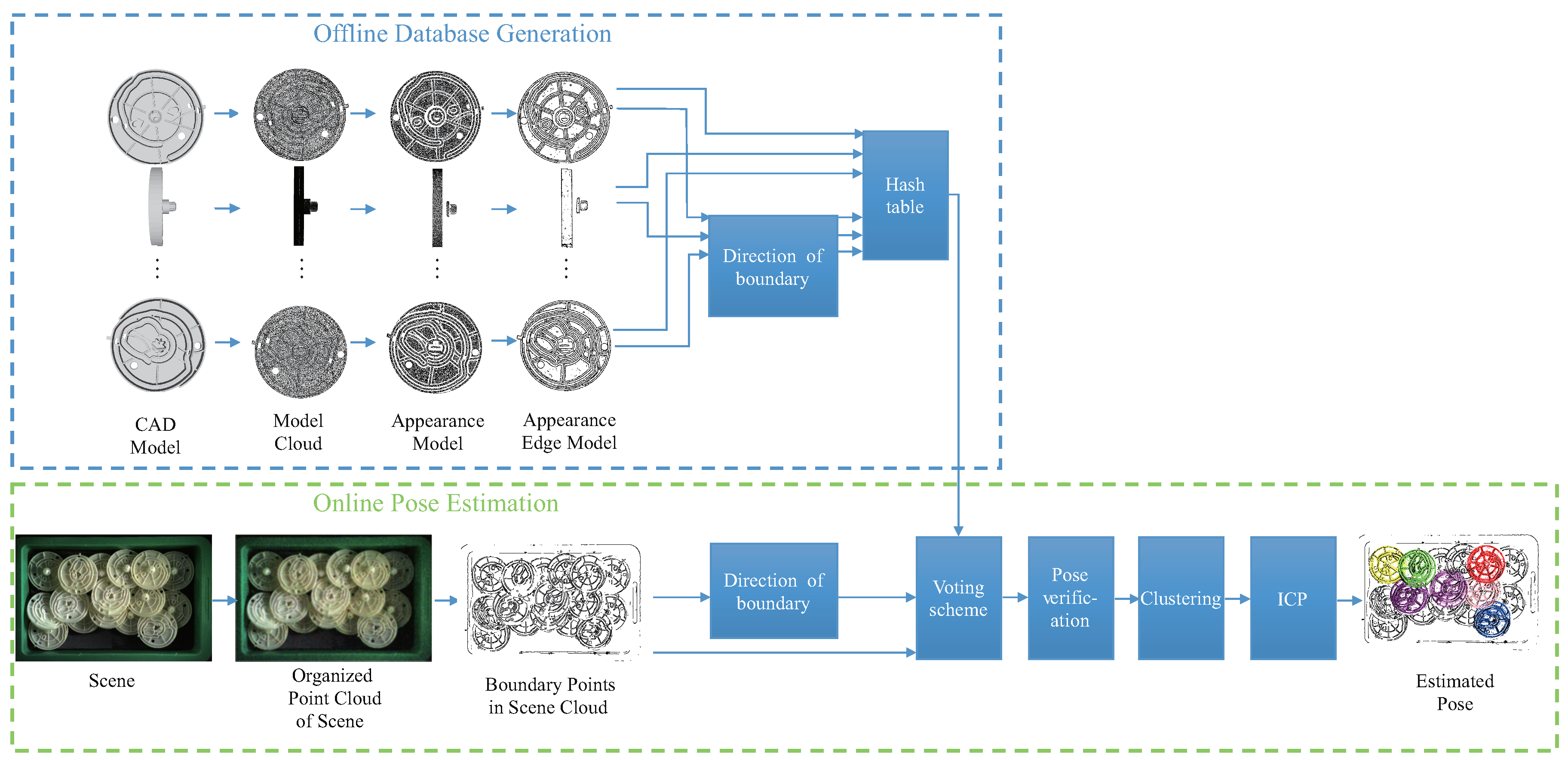
Figure 2.
The full Point Pair Feature (PPF)-MEAM pipeline. This algorithm could be divided into two phases. In the offline phase, a database is constructed using the target model. In the online phase, the pose of target part is estimated using the organized point cloud of the scene.
Figure 2.
The full Point Pair Feature (PPF)-MEAM pipeline. This algorithm could be divided into two phases. In the offline phase, a database is constructed using the target model. In the online phase, the pose of target part is estimated using the organized point cloud of the scene.
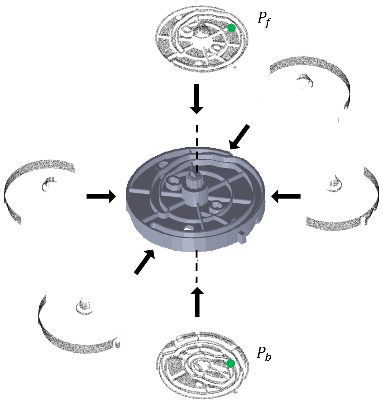
Figure 3.
Visible points extracted from six view points. Points and are located at two different sides of the part, which cannot be seen simultaneously. However, this point pair (, ) is calculated, and the PPF is stored in the hash table in other PPF-based methods.
Figure 3.
Visible points extracted from six view points. Points and are located at two different sides of the part, which cannot be seen simultaneously. However, this point pair (, ) is calculated, and the PPF is stored in the hash table in other PPF-based methods.
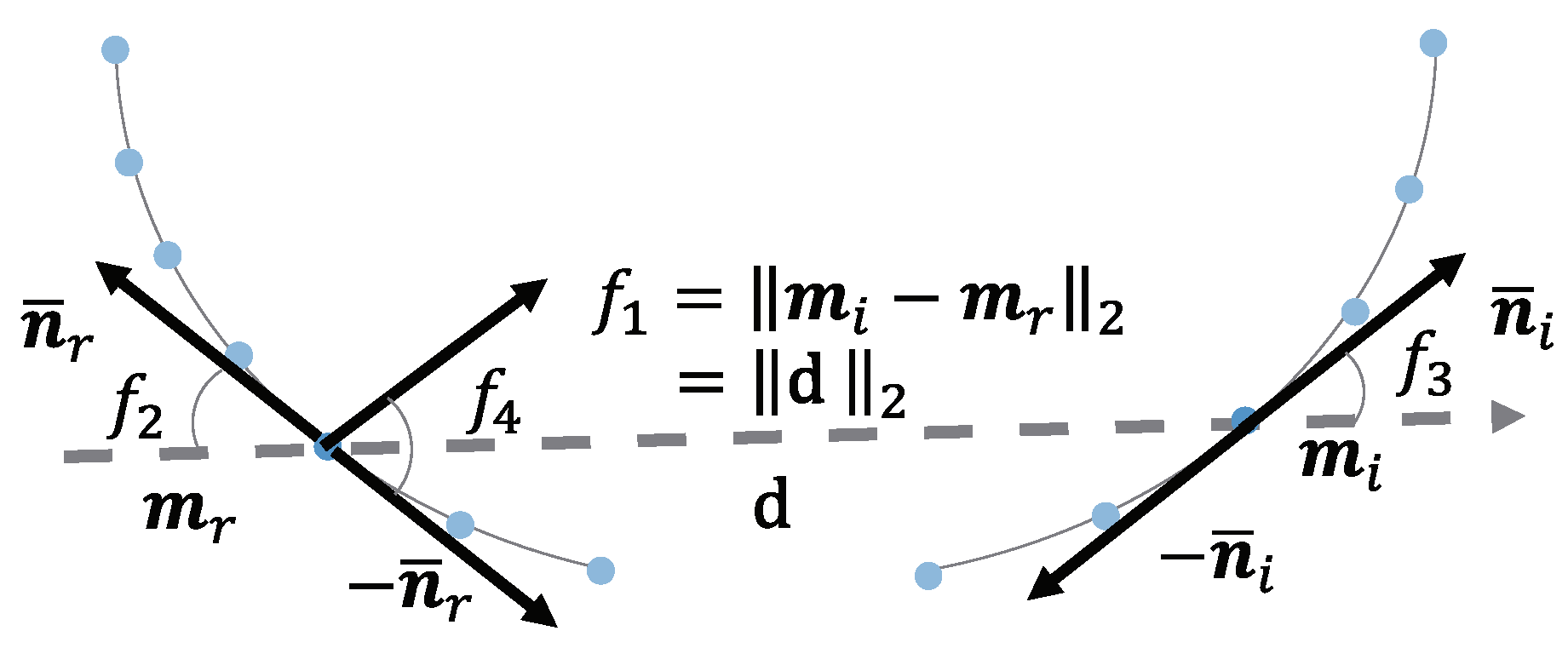
Figure 4.
The definition of the B2B-TL feature. This feature is different from the other PPF because it is using the points not only on the line segments, but also on the curves. A line cannot be fitted for the point on a curve, but the tangent line can be calculated and its direction used as the direction of the point.
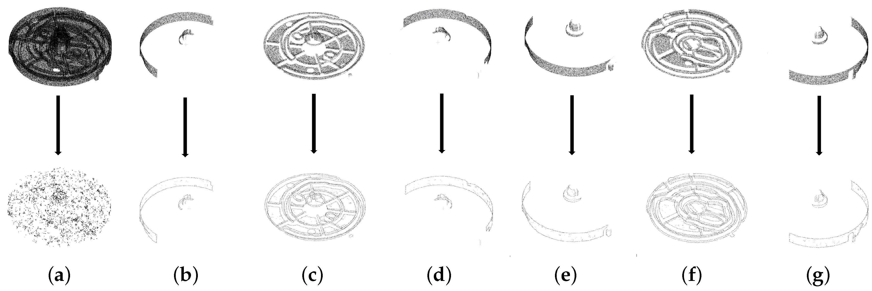
Figure 5.
Comparison between the boundary extraction using the original model and multiple appearance models. (a) shows extracted boundary points using the original model, that is, the model with all points around the part. (b,c,d,e,f,g) show extracted boundary points using multiple appearance models. Multiple appearance models outperform the original model in terms of boundary extraction.
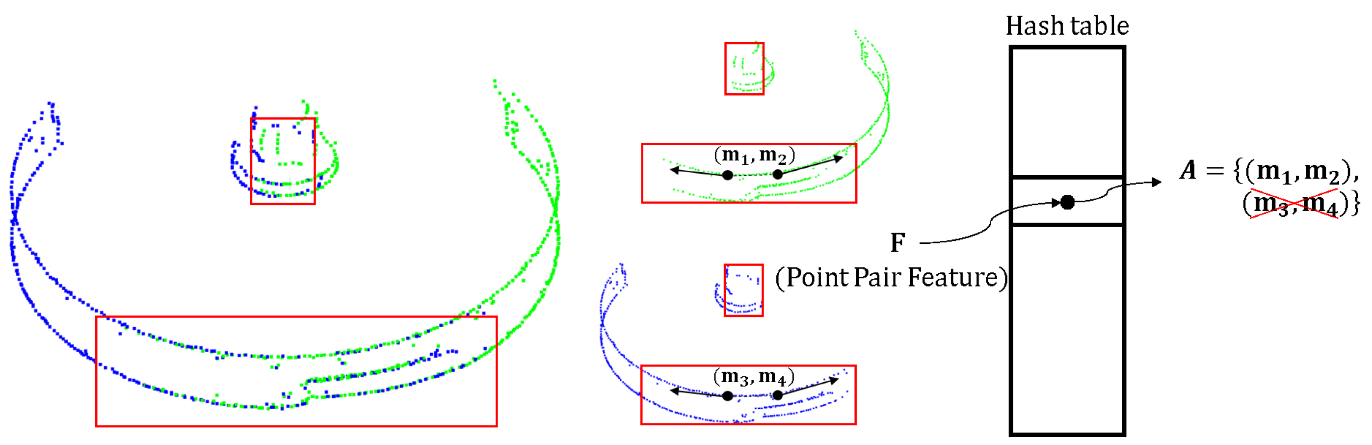
Figure 6.
Save the same point pairs only once in the hash table. The appearance edge models in green and blue are extracted from different viewpoints. These two appearance edge models share some of the same points, as shown in the red box. The point pair and is the same point pair in reality, but their points have different indices because they belong to different appearance models. Using the proposed encoding method, we recognized that these two point pairs are located at the same position and that only one pair needed to be saved in the hash table.
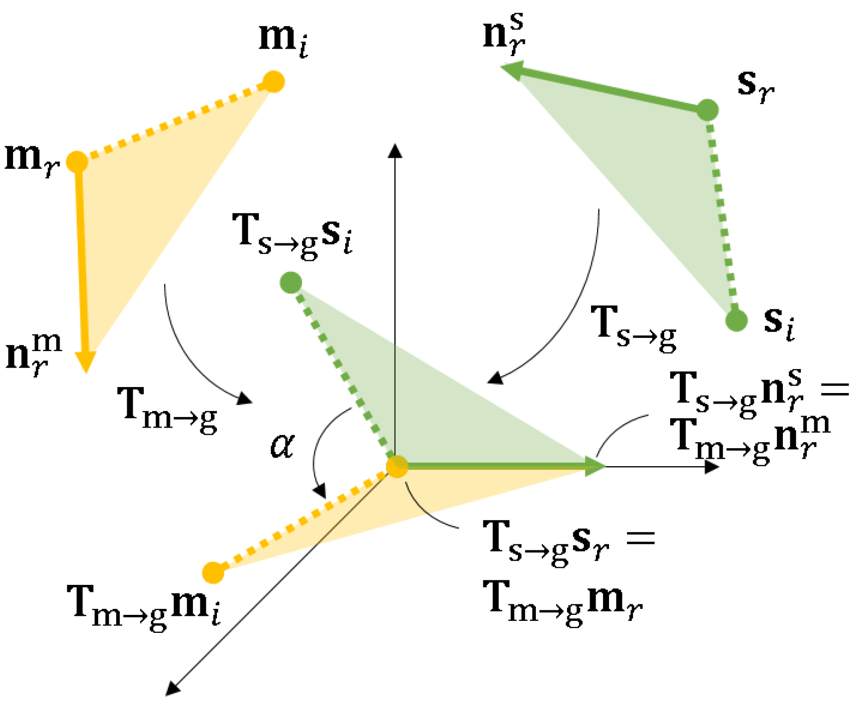
Figure 7.
Transformation between the model and scene coordinates. transforms the scene reference point to the origin and aligns its direction to the x-axis of the intermediate coordinate system. The model reference point and its direction are transformed similarly by . Rotating the transformed referred scene point with angle around the x-axis aligns it with the transformed referred model point . (, ) is then used to cast a vote in the 2D space.
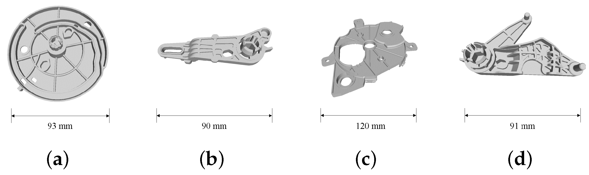
Figure 8.
Industrial parts used to verify the proposed method. We named these parts as Part A (a), Part B (b), Part C (c) and Part D (d). They are made of resin and used in a real car air-conditioning system. The appearance of these parts is complex, making the pose estimation more difficult compared to cases in which the parts have primitive shapes.
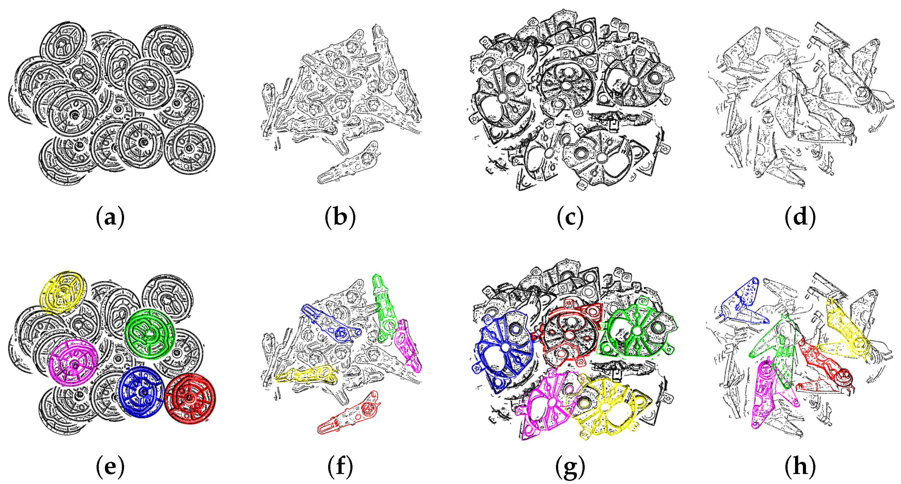
Figure 9.
(a,b,c,d) are the simulated scenes of the example parts. We estimated 5 poses in each scene, and (e,f,g,h) are the results of the pose estimation. The model point cloud is transformed to the scene space using the pose estimation results and rendered with different colors. These colors indicate the recommendation rank to grasp the part after considering occlusion. Models 1–5 are rendered in red, green, blue, yellow and pink, respectively.
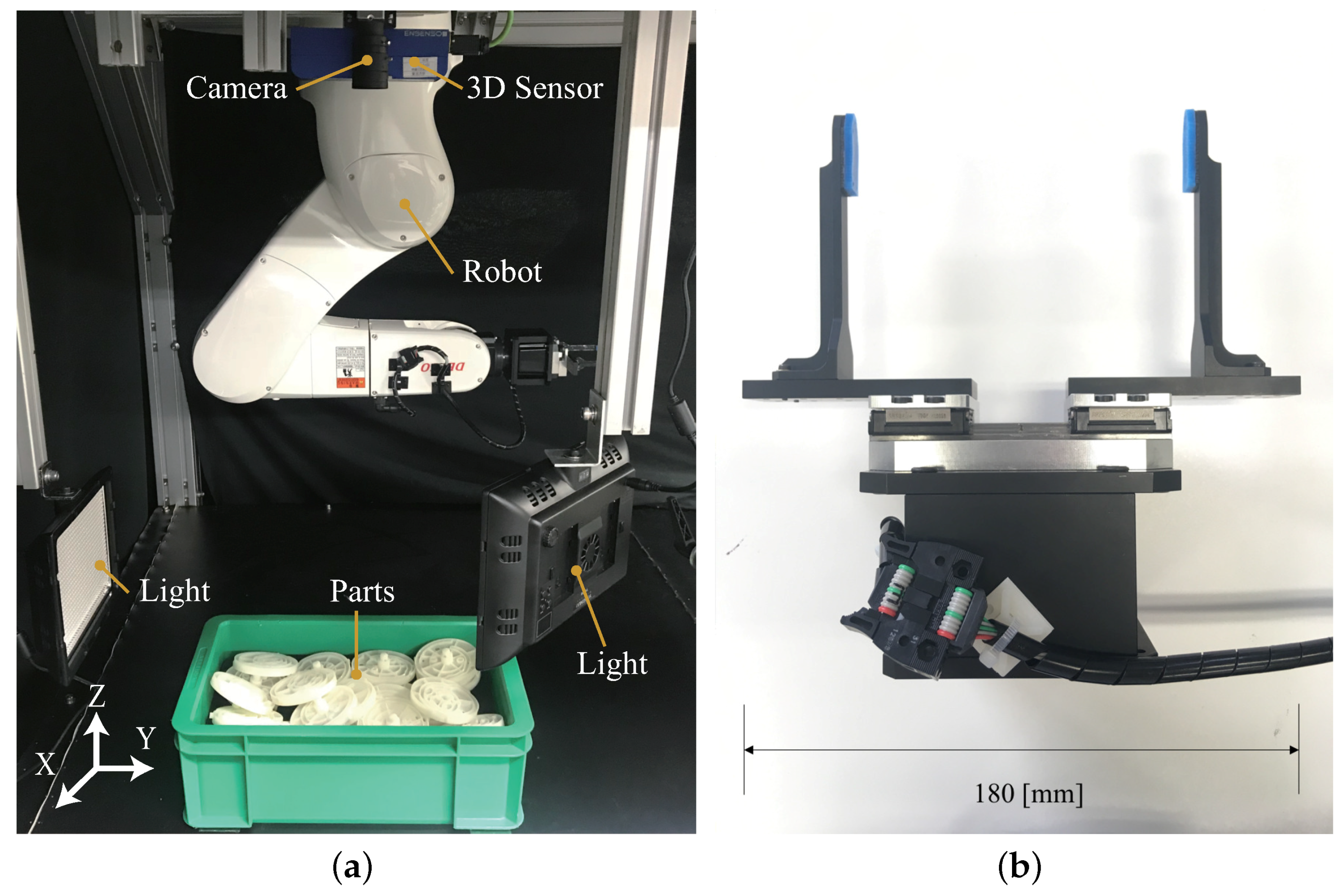
Figure 10.
The experimental system (a) was used to verify the proposed method. A color camera and 3D sensor were mounted on top (above the parts). To mitigate the effect of shadow on edge extraction, we installed two Light-Emitting Diodes (LEDs) on both sides of the box. A robot was used to perform the picking task with the gripper, as shown in (b).
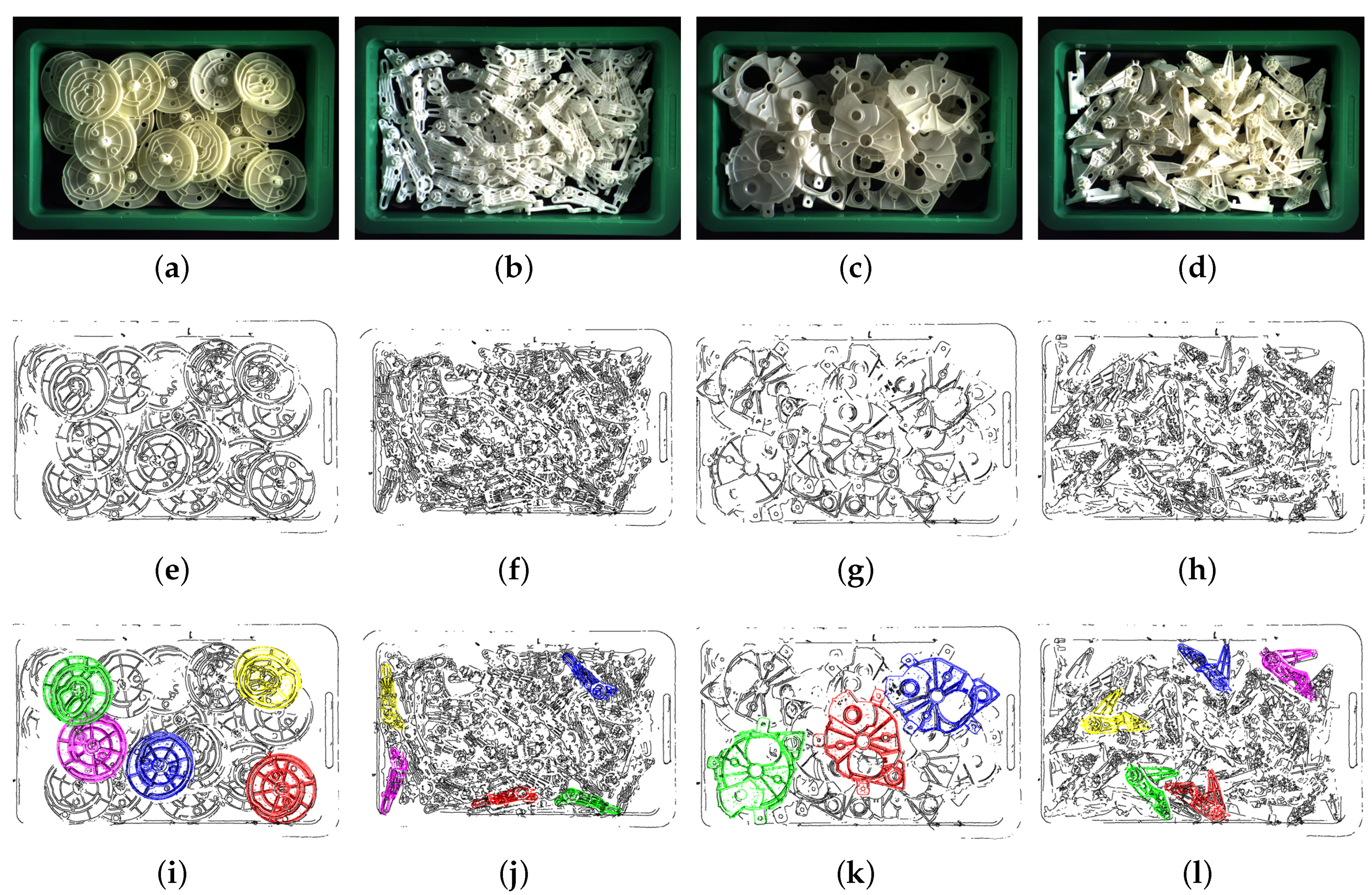
Figure 11.
(a,b,c,d) are the real scenes of the example parts. (e,f,g,h) are the boundary points of the scene cloud. (i,j,k,l) are the results of pose estimation. The model point clouds are transformed to the scene space using pose results and rendered with different colors. These colors indicate the recommendation rank to grasp the part after considering the occlusion. Models 1–5 are rendered as red, green, blue, yellow and pink, respectively.
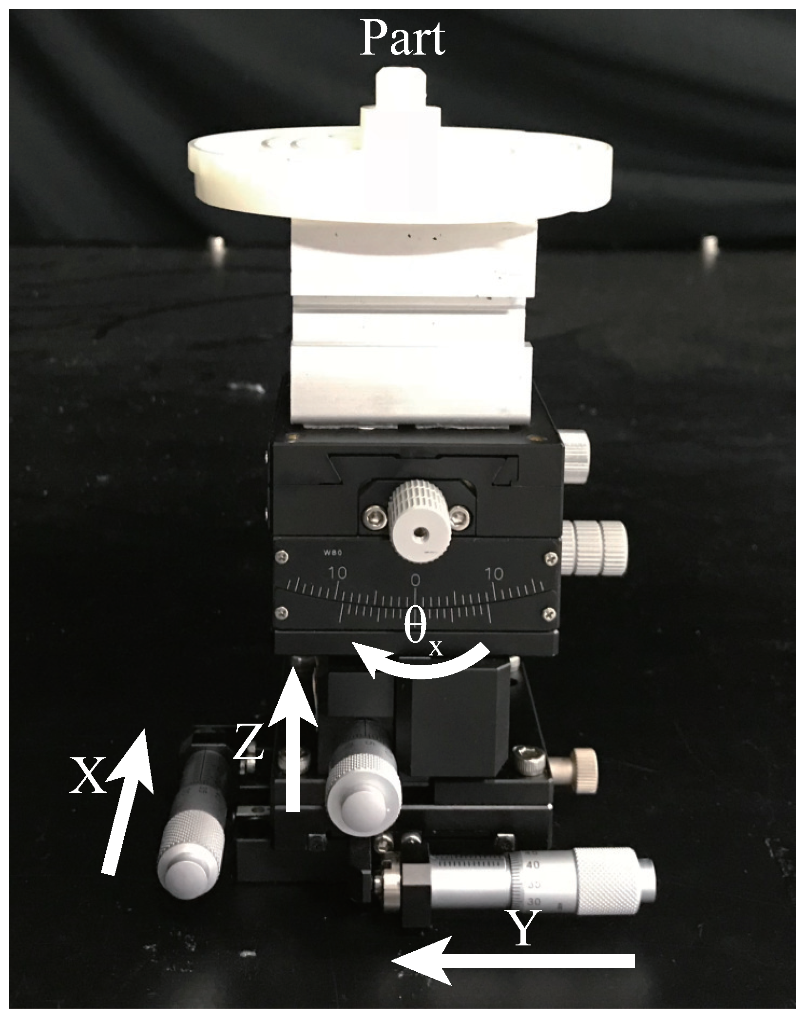
Figure 12.
The multi-axis stage unit is used to evaluate the relative error of pose estimation. After fixing the part on the top of the stage, we could move the part along each axis with a precision of 0.01 mm and rotate it by with a precision of .
Figure 12.
The multi-axis stage unit is used to evaluate the relative error of pose estimation. After fixing the part on the top of the stage, we could move the part along each axis with a precision of 0.01 mm and rotate it by with a precision of .
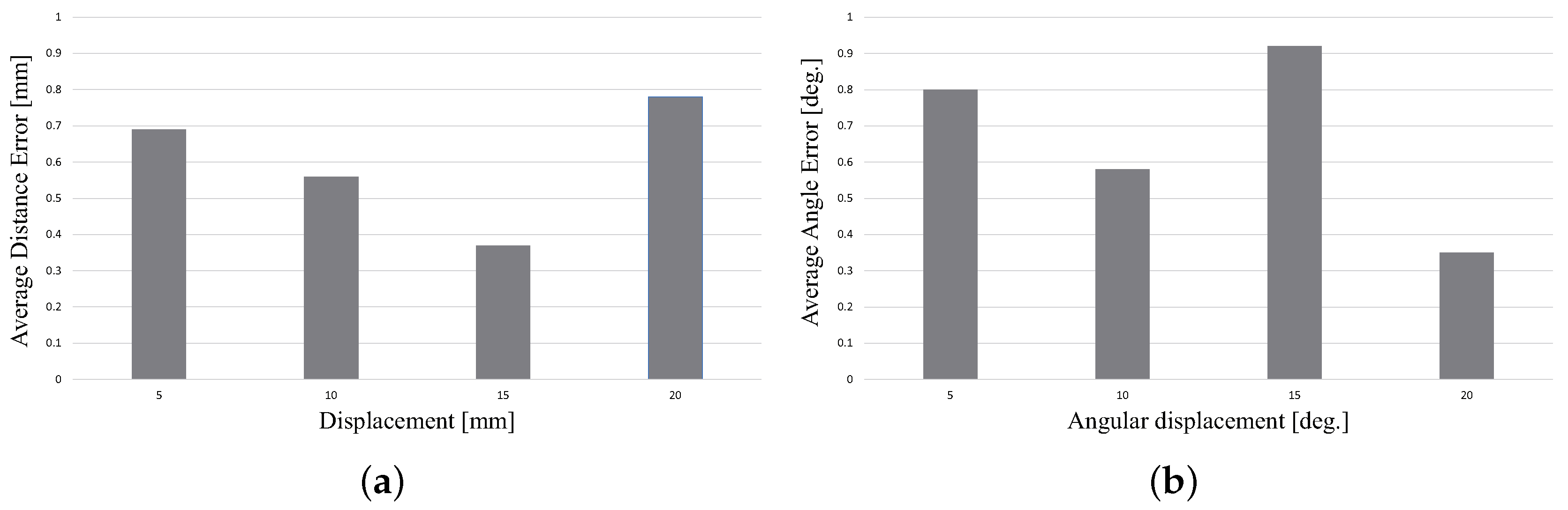
Figure 13.
(a,b) are the results of the relative error experiment. The part is moved by 5 mm, 10 mm, 15 mm and 20 mm using the stage. Pose estimation was performed each time we moved it. The moved distance was calculated by comparing the differences in the pose results. We conducted 10 trials for one part, and the average distance error is shown in (a). Similarly, we rotated the part by , , and , and the corresponding results are shown in (b).
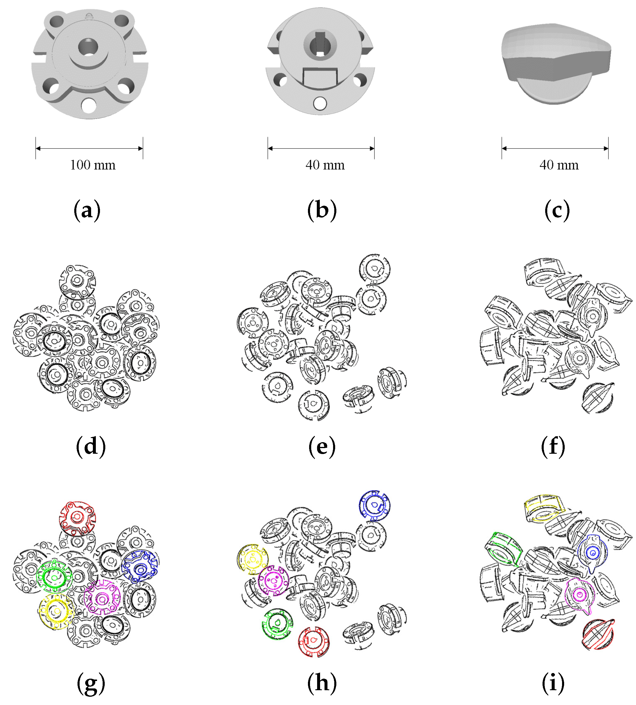
Figure 14.
Industrial parts in the Tohoku University 6D Pose Estimation Dataset. (a,b,c) are named as Part 1, Part 2 and Part 3, respectively. The example synthetic scenes are shown in (d,e,f). (g,h,i) are the results of the pose estimation.
Figure 14.
Industrial parts in the Tohoku University 6D Pose Estimation Dataset. (a,b,c) are named as Part 1, Part 2 and Part 3, respectively. The example synthetic scenes are shown in (d,e,f). (g,h,i) are the results of the pose estimation.
Table 1.
Recognition rate of the algorithms for synthetic scenes.
Table 1.
Recognition rate of the algorithms for synthetic scenes.
| Methods | Part A | Part B | Part C | Part D | Average |
|---|
| Proposed Method | 100% | 99.3% | 100% | 100% | 99.8% |
| Original PPF [12] | 49% | 66% | 71.3% | 90% | 69.2% |
Table 2.
Speed of the algorithms for synthetic scenes (ms/scene).
Table 2.
Speed of the algorithms for synthetic scenes (ms/scene).
| Methods | Part A | Part B | Part C | Part D | Average |
|---|
| Proposed Method | 1276 | 401 | 987 | 892 | 889 |
| Original PPF [12] | 3033 | 1470 | 1754 | 4430 | 2671 |
Table 3.
Recognition rate of the algorithms for real scenes.
Table 3.
Recognition rate of the algorithms for real scenes.
| Methods | Part A | Part B | Part C | Part D | Average |
|---|
| Proposed Method | 97% | 97% | 98.3% | 97% | 97.2% |
| Original PPF [12] | 8% | 72% | 58.3% | 89% | 57% |
Table 4.
Speed of the algorithms for real scenes (ms/scene).
Table 4.
Speed of the algorithms for real scenes (ms/scene).
| Methods | Part A | Part B | Part C | Part D | Average |
|---|
| Proposed Method | 1322 | 1353 | 1271 | 1360 | 1326 |
| Original PPF [12] | 2752 | 3673 | 1765 | 1438 | 2407 |
Table 5.
Comparison experiment for different N.
Table 5.
Comparison experiment for different N.
| N | 1 | 2 | 6 | 14 |
|---|
| Recognition rate | 69% | 93% | 97% | 95% |
| Time (ms/scene) | 942 | 1140 | 1322 | 3560 |
Table 6.
Comparison experiment using Part A.
Table 6.
Comparison experiment using Part A.
| | Proposed Method | Proposed Method without MEAM | Original PPF [12] |
|---|
| Recognition rate | 97% | 91% | 8% |
| Time (ms/scene) | 1322 | 2710 | 2752 |
Table 7.
Recognition rate of the algorithms verified on the Tohoku University 6D Pose Estimation Dataset.
Table 7.
Recognition rate of the algorithms verified on the Tohoku University 6D Pose Estimation Dataset.
| Methods | Part 1 | Part 2 | Part 3 | Average |
|---|
| Proposed Method | 96.7% | 97.3% | 100% | 98% |
| Original PPF [12] | 92% | 96.7% | 100% | 96.2% |
Table 8.
Speed of the algorithms verified on the Tohoku University 6D Pose Estimation Dataset (ms/scene).
Table 8.
Speed of the algorithms verified on the Tohoku University 6D Pose Estimation Dataset (ms/scene).
| Methods | Part 1 | Part 2 | Part 3 | Average |
|---|
| Proposed Method | 1982 | 1074 | 564 | 1207 |
| Original PPF [12] | 2034 | 1096 | 540 | 1223 |
Table 9.
Pickup success rate for Part A.
Table 9.
Pickup success rate for Part A.
| Total number of trials | Success | Failure | Success rate |
|---|
| 63 | 60 | 3 | |


