Analyte Quantity Detection from Lateral Flow Assay Using a Smartphone


1
Department of Electrical & Computer Engineering, Texas Tech University, Lubbock, TX 79409, USA
2
Infectious Disease Research Center, Korea Research Institute of Bioscience and Biotechnology (KRIBB), 125 Gwahak-ro, Yuseong-gu, Daejeon 34141, Korea
3
Nanobiotechnology and Bioinformatics (Major), University of Science & Technology (UST), 125 Gwahak-ro, Yuseong-gu, Daejeon 34141, Korea
*
Authors to whom correspondence should be addressed.
†
These authors contributed equally to this work.
Sensors 2019, 19(21), 4812; https://0-doi-org.brum.beds.ac.uk/10.3390/s19214812
Submission received: 24 October 2019
/
Revised: 29 October 2019
/
Accepted: 30 October 2019
/
Published: 5 November 2019
(This article belongs to the Section Biosensors)
Abstract
:Lateral flow assay (LFA) technology has recently received interest in the biochemical field since it is simple, low-cost, and rapid, while conventional laboratory test procedures are complicated, expensive, and time-consuming. In this paper, we propose a robust smartphone-based analyte detection method that estimates the amount of analyte on an LFA strip using a smartphone camera. The proposed method can maintain high estimation accuracy under various illumination conditions without additional devices, unlike conventional methods. The robustness and simplicity of the proposed method are enabled by novel image processing and machine learning techniques. For the performance analysis, we applied the proposed method to LFA strips where the target analyte is albumin protein of human serum. We use two sets of training LFA strips and one set of testing LFA strips. Here, each set consists of five strips having different quantities of albumin—10 femtograms, 100 femtograms, 1 picogram, 10 picograms, and 100 picograms. A linear regression analysis approximates the analyte quantity, and then machine learning classifier, support vector machine (SVM), which is trained by the regression results, classifies the analyte quantity on the LFA strip in an optimal way. Experimental results show that the proposed smartphone application can detect the quantity of albumin protein on a test LFA set with 98% accuracy, on average, in real time.
1. Introduction
Lateral flow assay (LFA) [1] strips are widely used for analyte detection in a given liquid sample. This technology has rapidly gained interest nowadays due to its low-cost, simple, and swift detection of biochemical compounds in samples [2,3,4]. Specifically, LFA pads are cellulose-based strips containing specific reagents which are activated when the target analyte is present in the sample. LFA has been adopted in various fields of study, e.g., point of care [5,6], agriculture [7], food [8], medicine, and environmental science [9]. Moreover, LFA is important for diagnosis, such as pregnancy, heart failure [10], contamination [11], and detection of drugs of abuse [12]. Some of these LFAs are particularly designed for point of care testing [13,14].
Existing analyte detection methods using LFA strips can be categorized into qualitative and quantitative approaches [15]. Qualitative analysis is performed by assessing colors at the region of interest (ROI) visually [13]. This rapid result of qualitative tests helps make immediate decisions. However, qualitative analysis provides subjective judgement and may give a wrong interpretation [16]. Hence, quantitative methods are needed where the results are not clear with qualitative analysis. Quantitative analysis of LFA is shown to facilitate point-of-care testing compared to qualitative analysis [16,17,18,19]. Quantitative approaches require a method that can readily deliver quantitative measurements in a fast and accurate way. Due to their superior processing ability and portability, smartphones are being used for acquiring and processing biomedical signals and images [20,21,22]. Existing quantitative analysis requires external devices [23,24] in addition to a smartphone, such as an external lens, LFA housing device, or LED strip/optical fiber. Standalone devices [25] adopt specific processors, light sources, and housing for the LFA strip and are configured to exclusively perform analyte quantity detection [26,27]. For automated quantification and rapid decision, a mobile camera–based LFA detection method has been highlighted, which adopts specific lighting conditions [28] or external housing attached to a smartphone [23] for LFA detection.
For quantification of the result, optical strip readers are commonly attached to a smartphone. Images of the strips are captured with the smartphone camera, and then the optical strip reader processes the image using image processing software that does, for example, threshold-based color segmentation [29] to quantitatively measure the amount of analyte present in the sample. This procedure requires placing the LFA and light source precisely when the smartphone captures the image and also needs proper illumination for high contrast between ROI and background, which is not always easy to achieve [30]. In order to provide more accurate quantitative analysis, an LFA analyte detection system that is resilient at diverse illumination conditions needs to be developed [4]. A smartphone-based automated method quantifying the quantity of the analyte present in a sample can be promising due to its portability and ease-of-use.
Several techniques have been adopted for analyte detection in LFA, and recent smartphone-based detection techniques are highlighted. Carrio et al. [12] and Cooper et al. [28] demonstrated that smartphone-based LFA detection can be applied to the quantification of drugs of abuse. However, these methods require devices other than a smartphone. In this paper, we propose a novel smartphone-based analyte quantity detection method for an LFA strip, which detects the amount of analyte in an LFA strip using a smartphone without an external device. We also design the proposed method to be resilient at diverse lighting conditions. Using optical methods, the application can easily detect test line and control line pixels’ intensity values without using an external strip reader device, which increases portability and convenience. Unlike a standalone LFA strip reader device, our developed system is portable, accurate, and convenient. Using an image processing technique, this application can replace a cumbersome reader device and effectively measure the presence of the analyte in a sample liquid in a quantitative way. Compared to the conventional technologies, our proposed method maintains its estimation performance under diverse lighting conditions without requiring an external LFA housing device. The main contributions of this paper are summarized as follows:
- A convenient and portable alternative to read LFA strips using solely a smartphone. The conventional techniques require external devices. Our proposed method uses a novel smartphone application that instantly detects an analyte quantity in an LFA strip without any prior calibration or any requirement of an external device.
- Resilience at various light conditions in detecting the analyte amount in an LFA strip. The performance of existing techniques is affected by the environment such as lighting conditions. Our proposed algorithm can accurately estimate the quantity of the analyte in an LFA strip in diverse lighting conditions.
2. Materials
2.1. Input Data: LFA Pads
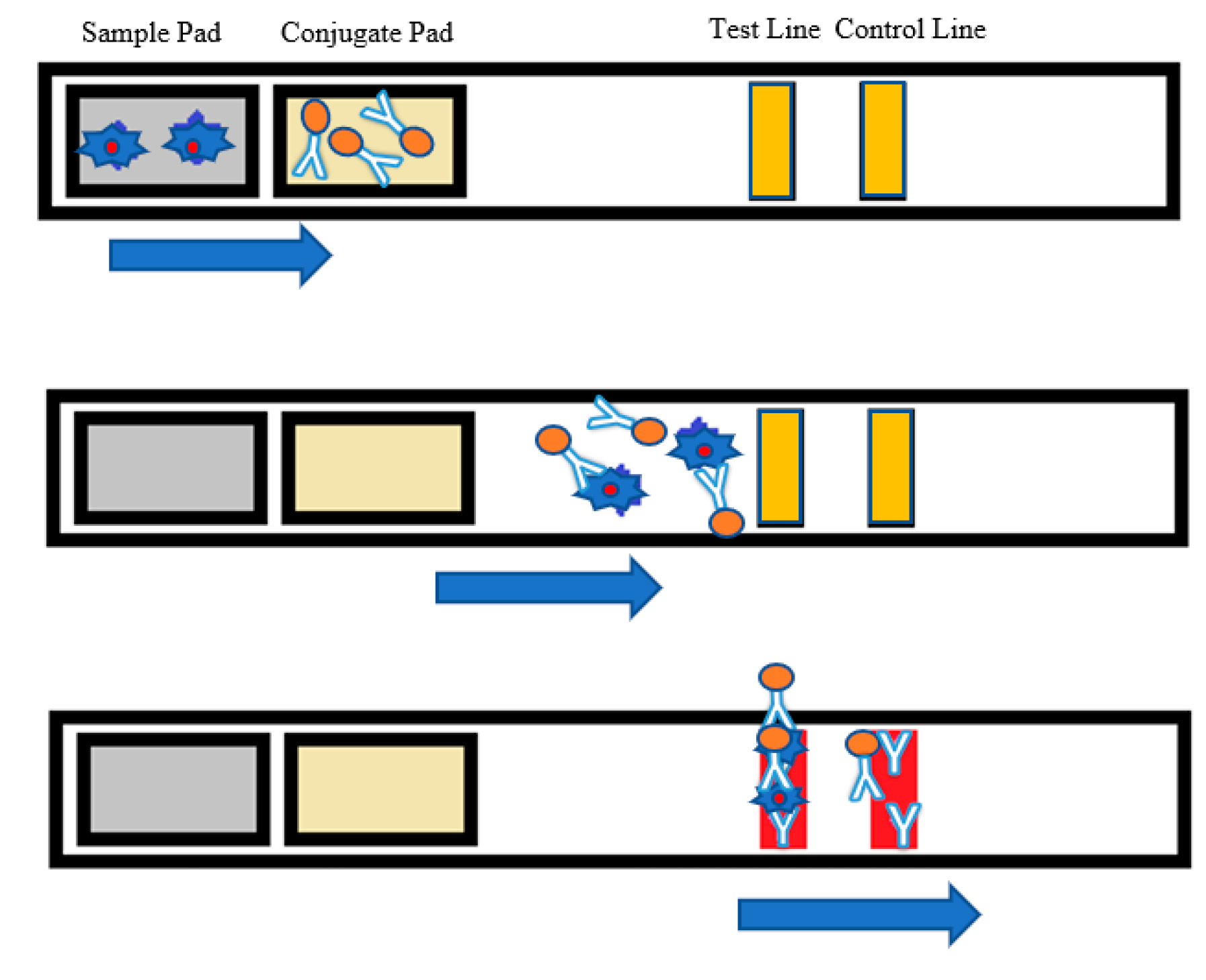
An LFA strip contains four primary parts—sample pad, conjugate pad, membrane, and absorbent pad [31]. The sample pad is the region where the sample solution is distributed. The sample solution is designed to flow from the sample pad to the conjugate pad, which contains the conjugate labels (i.e., gold nanoparticles) and antibodies. Figure 1 shows the architecture and working principle of an LFA strip. The conjugate tags bind to the analyte molecules of the sample solution and flow along the strip. The membrane is made of nitrocellulose material. As the sample moves along, reagents situated on the test lines of the porous membrane capture the conjugated labels bound to the target analyte. The control line on the membrane consists of specific antibodies for the particular conjugate and captures the conjugate tags. These phenomena are observed as the red color in the test/control lines. The color intensity of the test line is expected to vary proportionally to the quantity of the analyte in the test sample. However, there is no color change in the test line if the target analyte is absent in the sample. A colored control line assures that the test has been performed well [32], as shown in Figure 1.
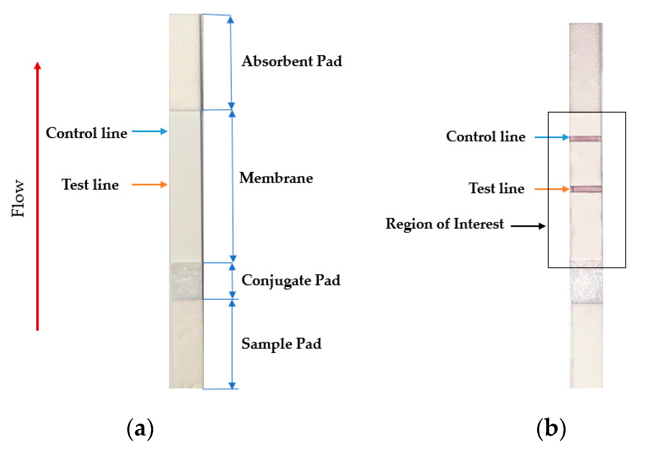
The analyte quantity in the sample is expected to be proportional to the intensity of the red colored test line region. Hence, a weighted summation of red color in the test line region can be considered as the parameter for the detection of analyte quantity, where the weight is considered to be the color intensity of each pixel. Figure 2a shows a sample LFA test strip with its consisting parts, while Figure 2b shows the ROI (see rectangular box) and the test and the control lines (see orange and blue lines).
2.2. Data Acquisition Using a Smartphone Camera
LFA strips of known quantities of target analyte on sample pads were obtained from the Korea Research Institute of Bioscience & Biotechnology (KRIBB). The target analyte was albumin protein (albumin from human serum acquired from Sigma Aldrich, Saint Louis, MO, USA [33] with product number A9511), and the conjugate tags were gold nanoparticles with an albumin antibody. The solvent of pH 7.4 PBS (phosphate buffered saline, purchased from Gibco, Paisley, UK) was used to prepare 10 microliters (μL) of solution of albumin sample. Here, we considered the following five different concentration levels: 10 ng/mL, 1 ng/mL, 100 pg/mL, 10 pg/mL, and 1 pg/mL. Three sets of samples were available for the study, with each set containing five LFA strips having five different concentrations. As a result, the corresponding analyte quantities of five different concentration levels are 10 ng/mL × 10 μL = 100 pg, 1 ng/mL × 10 μL = 10 pg, 100 pg/mL × 10 μL = 1 pg, 10 pg/mL × 10 μL = 100 fg, and 1 pg/mL × 10 μL = 10 fg, respectively. An Institutional Review Board (IRB) assessment was not performed because the sample was purchased. Figure 3 shows sample images of LFA set #1. Each reading was taken five times to reduce error. Hence, a total of 15 LFA strips were used, and 75 readings were obtained in this study. Two sets, each consisting of five LFA strips of the aforementioned quantities (set #1 and #2), were used to train the machine learning model, and the other set was used for validating and testing the model of the proposed method. The data acquisition procedure was performed with an Android smartphone Samsung Galaxy S7 Edge, Samsung Electronics, Seoul, South Korea [34] with Android version 8.0.0. We used the rear camera of the smartphone, which had a maximum resolution of 12 megapixels (4032 × 3024 pixels). Autofocus function was enabled, and the flashlight was turned off during the data acquisition procedure. Images of the LFA strips were captured under different ambient lighting conditions in the laboratory. The room had a floor area of 41.475 m2 and was illuminated with a 36-Watt ceiling light and a 27-Watt table lamp, respectively. The method was evaluated based on acquired data using MATLAB 2018b, The MathWorks, Inc., Natick, Massachusetts, USA [35].
3. Methods
3.1. Feature Extraction
We considered the number of red pixels accumulated on the test line as a feature. We assumed that the cumulative sum of red pixels’ intensities in the test line varied proportionally with analyte quantity under a specific lighting environment. To extract this feature, we performed the following: (1) selecting the test line region and the control line region, (2) segmenting image via optimal thresholding using Otsu’s method [36], and (3) calculating weighted sum of red pixels’ intensities, which are explained in Section 3.1.1, Section 3.1.2, and Section 3.1.3, respectively. During all these steps, image preprocessing and machine learning techniques were applied as described in these sections.
3.1.1. Test and Control Line Region Selection
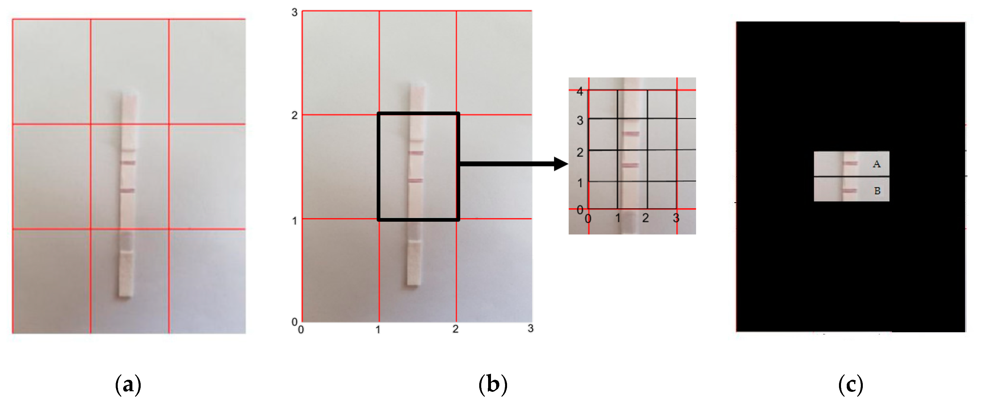
To extract the test and control line regions, the acquired image is cropped with fixed dimensions and a fixed aspect ratio [37]. This technology has been readily available in current generation cellular devices, and the procedure has been used in printing, extracting thumbnails, and framing digital pictures. Accurate placement of the LFA strip under the camera is required for exact approximation of analyte quantity. Figure 4a shows an example of an accurate placement of an LFA under a smartphone camera, where the ROI sits exactly in the center box of the 3 × 3 grid of the camera view. Then, the center grid region’s dimensions are readily extracted from the acquired LFA image. Figure 4b shows the indexes of the center box’s boundary points: ((1, 1), (2, 1), (1, 2), (2, 2)). The developed application automatically crops and extracts the test and control line regions from the center grid point locations of the image. The regions are obtained from inner grid indexes for the test line ((0, 1), (3, 1), (0, 2), (3, 2)) and the control line ((0, 2), (3, 2), (0, 3), (3, 3)). As shown in Figure 4c, the control line and the test line are identified as region A and region B, respectively. These regions are then considered for further calculation.
3.1.2. Image Segmentation via Optimal Thresholding Using Otsu’s Method
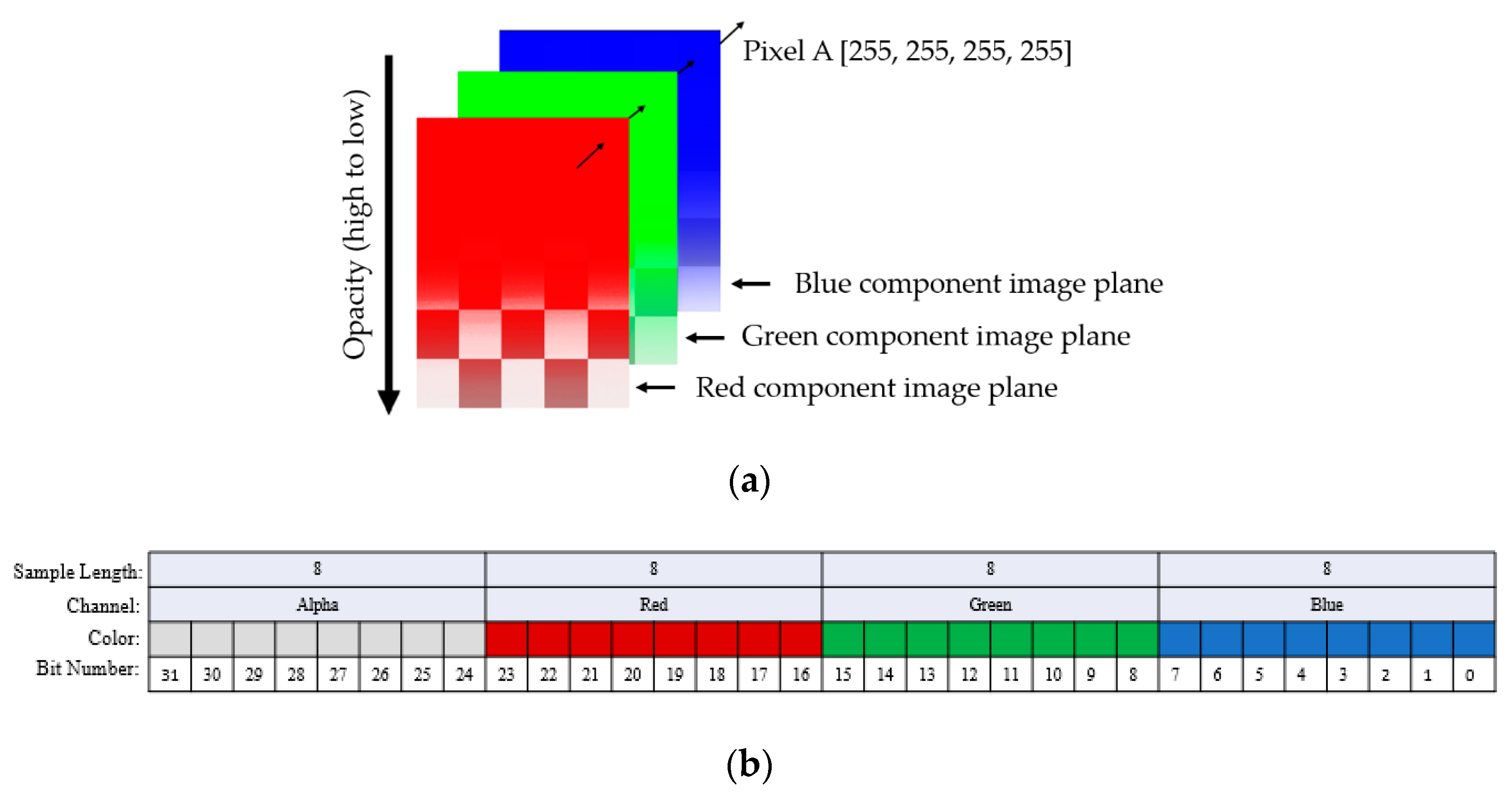
As mentioned in Section 2, we captured the LFA strip images using a Samsung Galaxy S7 smartphone camera with the resolution of 12 megapixels (4032 × 3024 pixels). The Samsung Galaxy S7 camera generated LFA images in Alpha-Red-Green-Blue (ARGB) 32-bit color space consisting of alpha (A), red (R), green (G), and blue (B) channels. Here, the A, R, G, and B channels represent opacity and red, green, and blue intensities, respectively. Figure 5a,b show the ARGB representation of an image and the 32-bit representation of a pixel in the image, respectively. Each pixel can have 232, or 4,294,967,296, different representations since a pixel is represented by 32 bits.
Denoting the red color intensity by and the green color intensity by , we observed that the ratio of red to green channel intensity was noticeably different near the test/control line regions compared to other regions as shown in Figure 6. Specifically, values for pixels of an LFA strip image were nearly unity except for the test and control line regions.
Otsu’s multilevel thresholding method [36,38] has been included in this paper, which thresholds an image automatically by minimizing variance of intra-class intensity level. This method was applied to the extracted control line to obtain an optimal threshold value for masking. This masking is used to only consider the ROI for calculation. This threshold value was applied to the whole image for creating the mask, which consists of points whose red to green channel intensity ratio values are higher than . Denoted by the mask intensity value at the pixel location , was calculated by the following equation:
Figure 7a has been obtained from MATLAB to visualize the color difference between the ROI and the non-ROI region. In the test and the control line regions of the image, the red intensity values (in the range near 160) are larger than the green intensity values (in the range near 130), while the other regions had comparable red and green intensity values. Evidently, the intensity ratio of red to green color channels showed a higher difference in the test and control line regions, i.e., a higher ) value. Using the optimal threshold (THmask), the mask image was obtained, which is shown in Figure 7b. Figure 7c shows the cropped final image of the selected control line and test line regions.
3.1.3. Calculation of the Weighted Sum of Red Pixels’ Intensities
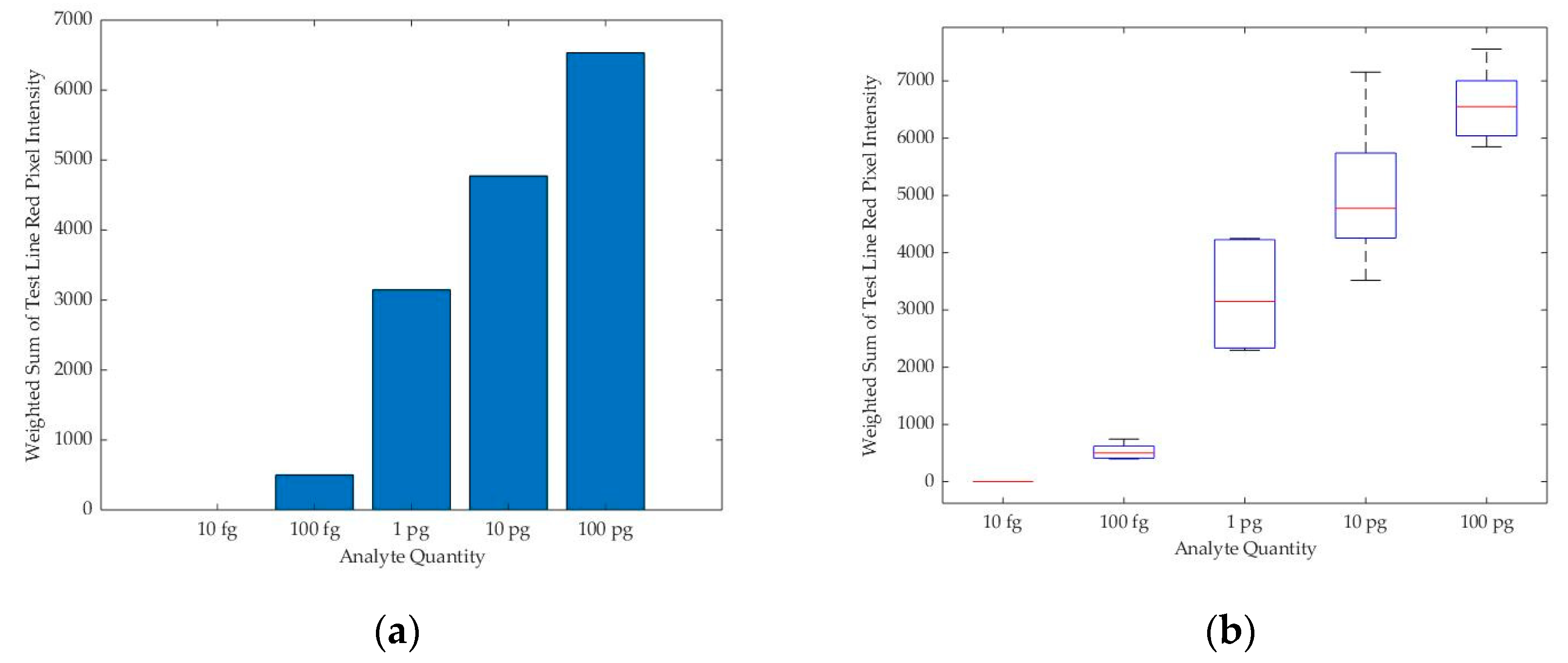
We observed that the sum of color intensities of the red pixels on the test line region tends to increase as the analyte quantity increases under a specific lighting environment, as shown in Figure 8. From this observation, we assumed that the counted red pixels’ intensity values on the test line from the captured smartphone camera image can estimate the analyte quantity from the LFA strip.
Equation (2) shows the method for calculating the weighted summation of red pixels’ intensity values in a region (Sregion).
This equation is applied throughout the extracted control and test line. By calculating the weighted summation of the red pixels’ intensity values of the control line and test line regions Scontrol and Stest were obtained from the masked image.
3.2. Multiclass Classification Using MachineLearning Techniques
3.2.1. Input Parameter for Classification (Test to Control Line Signal Intensity (T/C) Ratio)
The proposed method utilized a regression analysis [39,40] to approximate the analyte quantity and predict the value using machine learning techniques. As an input parameter for regression analysis, we considered the ratio of the test to control line signal intensity (T/C ratio), since the T/C ratio increase proportionally with analyte quantity despite of variation in illumination. The T/C ratio is expressed in Equation (3),
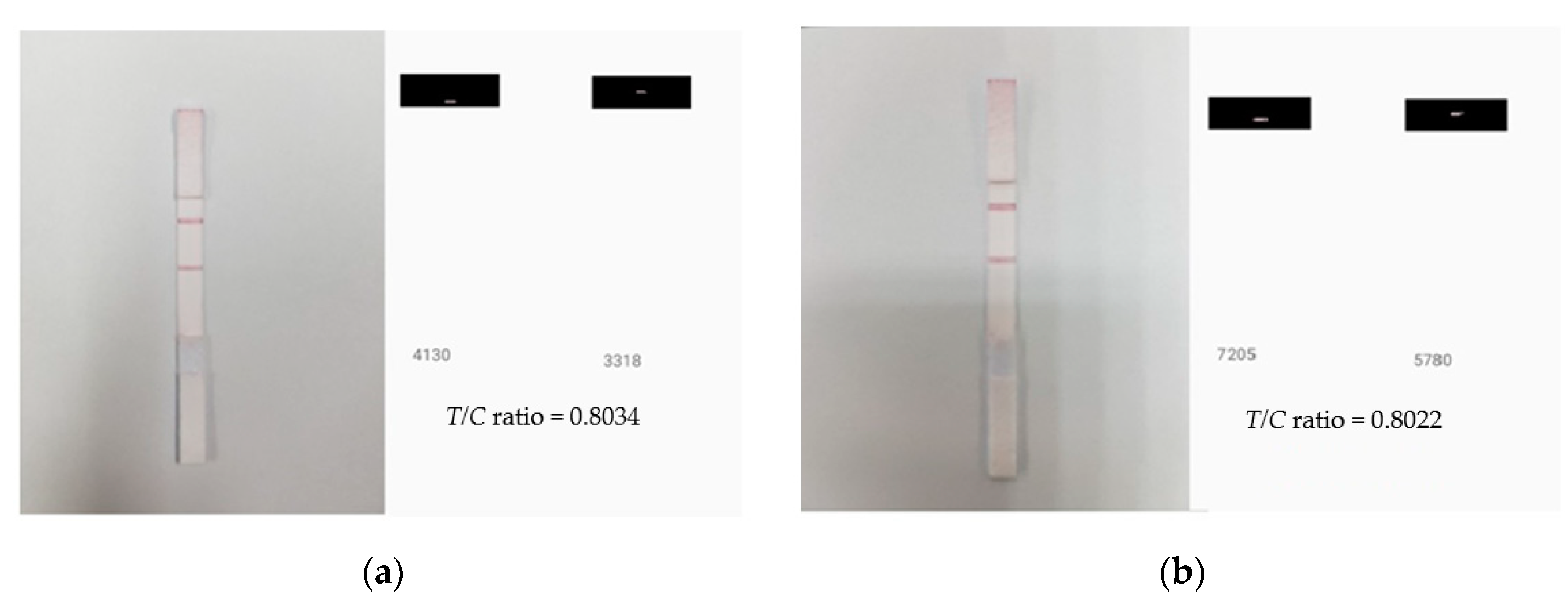
where Stest and Scontrol are the weighted sums of red pixels’ intensity values of the test and control lines, respectively. In this paper, we observed that the T/C ratio remained stable in different luminous environments for the same analyte quantity. Figure 9 shows two readings of the same LFA strip under two different ambient light environments. To simulate these two different lighting environments, a 36-Watt ceiling light and a 27-Watt table lamp light was used in a laboratory of 41.475 m2 floor area (see Section 2 for setup). The T/C ratios obtained had 0.15 percentage difference, which validates its ability as a classifier parameter since it is resilience at different light conditions.
3.2.2. Regression and Classification
Visual detection methods, which has been used to detect analyte quantity, are qualitative and erroneous due to absence of quantification parameters. From the conjugation of albumin with gold nanoparticle tags, a comparative valuation of quantifiable color density is possible. Figure 10 shows the box whisker plot of the acquired T/C ratios for different readings.
A regression analysis was performed based on the feature parameter (T/C ratio) from Table 1, Table 2 and Table 3. The approximations obtained from the regression analysis were utilized for classification into the categories mentioned in Section 2.2 using machine learning technique. A linear support vector machine (SVM) classifier [41] was adopted for the classification of analyte quantity categories. The input parameter for the SVM is the approximated quantities obtained from the regression analysis. After training the linear SVM classifier using two training LFA sets with known analyte quantities, the trained classifier estimates the analyte quantity of a test LFA set.
3.3. Developed Smartphone Application
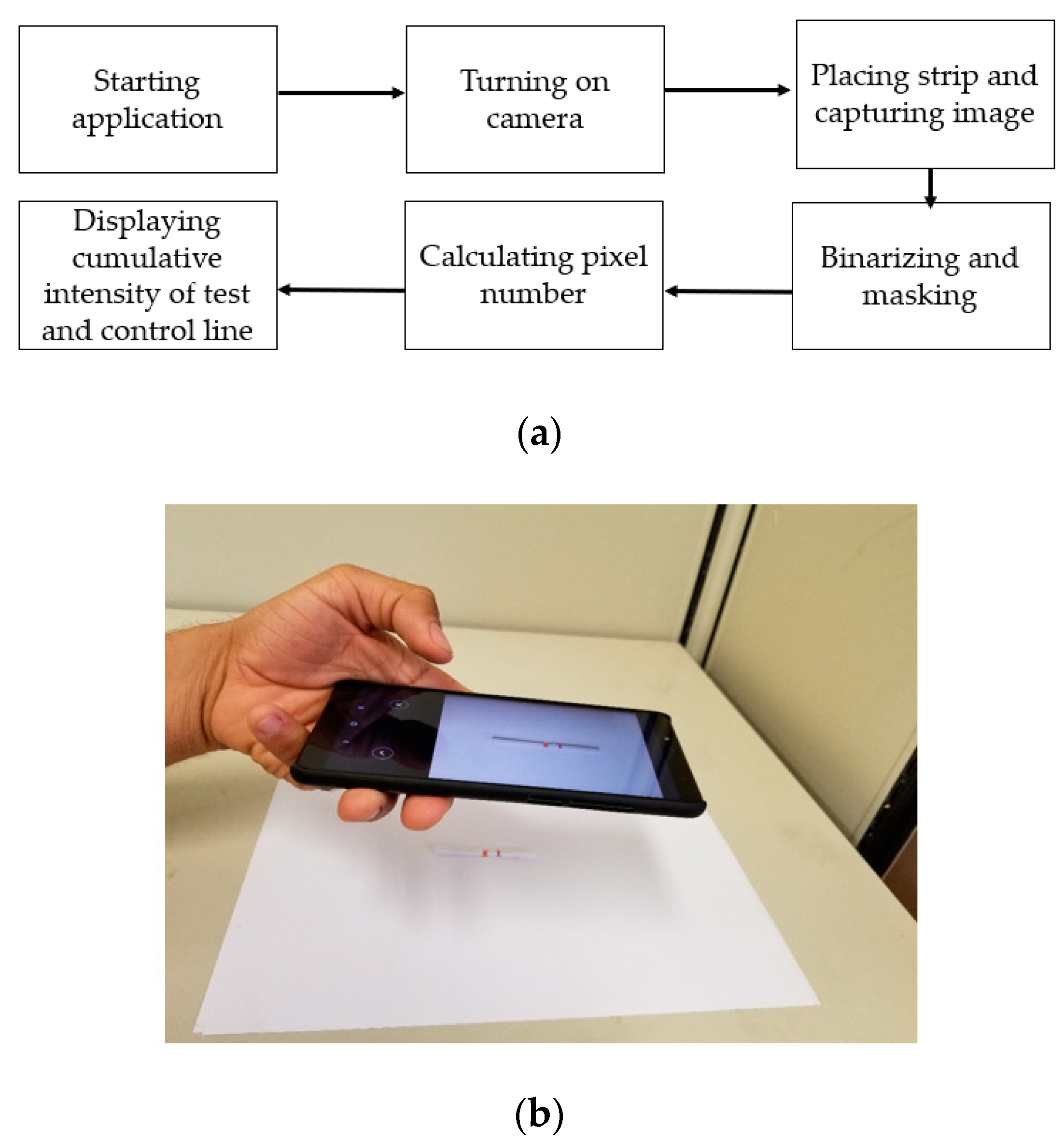
A smartphone application was developed on the Android platform following the proposed method described in Section 3.1 and Section 3.2. Figure 11a shows the flowchart of our developed application’s operation, and Figure 11b shows an example of data acquisition using our developed application.
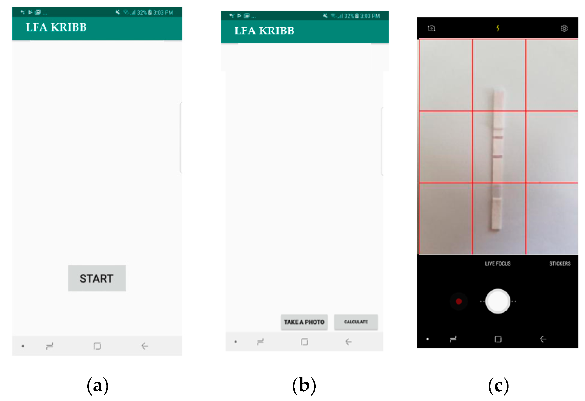
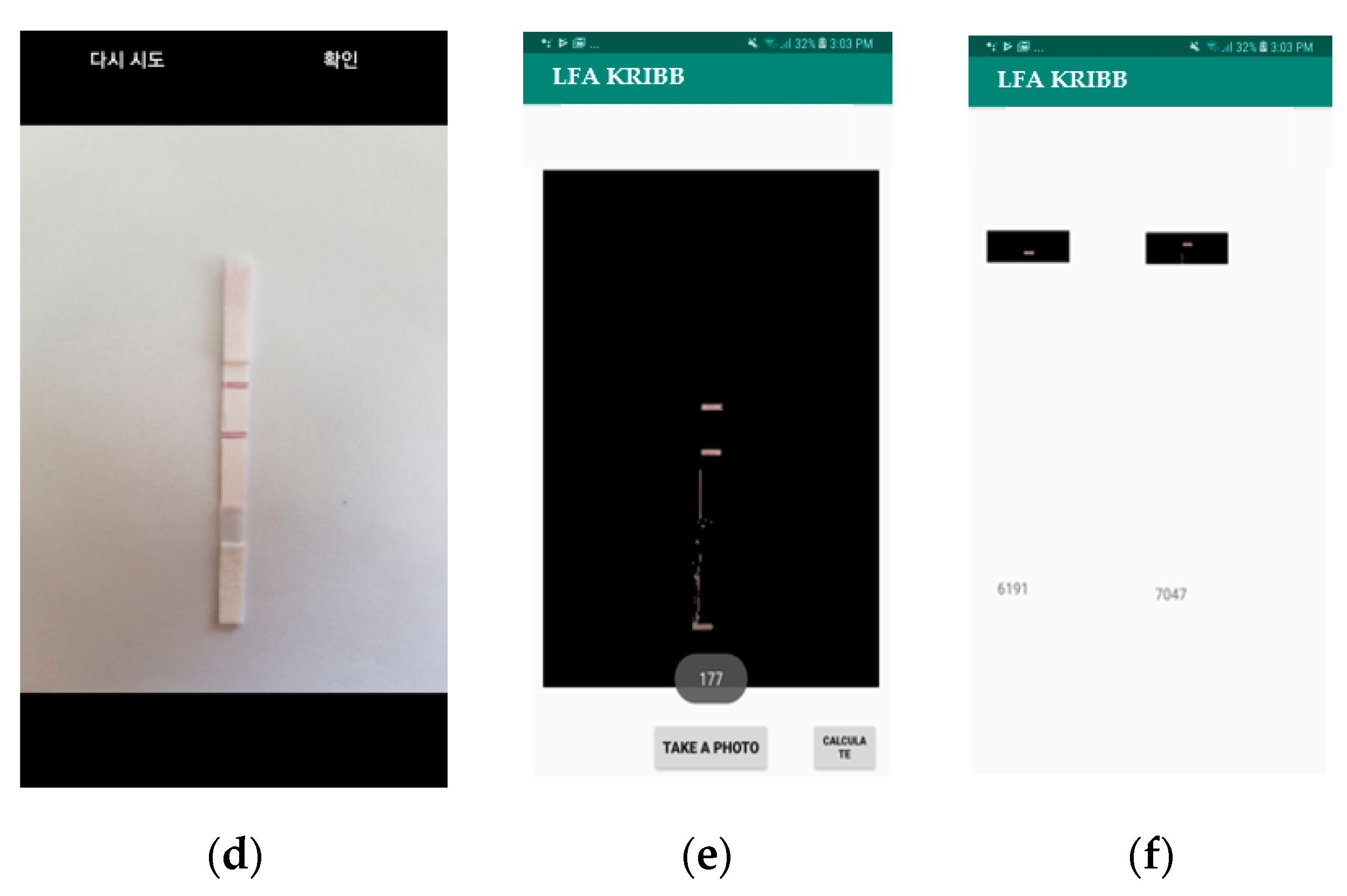
The smartphone application was tested on a sample LFA to evaluate the performance in a real-life scenario. The testing procedure was as follows: a test strip was placed under the smartphone on a white background. Using the grid view of the camera, the ROI was positioned inside the center box. The image was captured, and the ROI was obtained. The application then created a mask using the preprocessing technique mentioned in the proposed algorithm. In the masked region, the weighted sums of red pixels’ intensities of the test and the control line regions were calculated. Then, T/C ratio values that corresponded to the quantity of the analyte were calculated. Figure 12 shows the application screens and steps of operation of an LFA strip with a 100 pg analyte quantity. Figure 12c shows the positioning of the LFA strip in the center box of the grid view. Figure 12e shows the test and control line with the number of pixels in the mask, and Figure 12f shows the weighted sums of red pixels’ intensities of the control line (6191) and test line (7047).
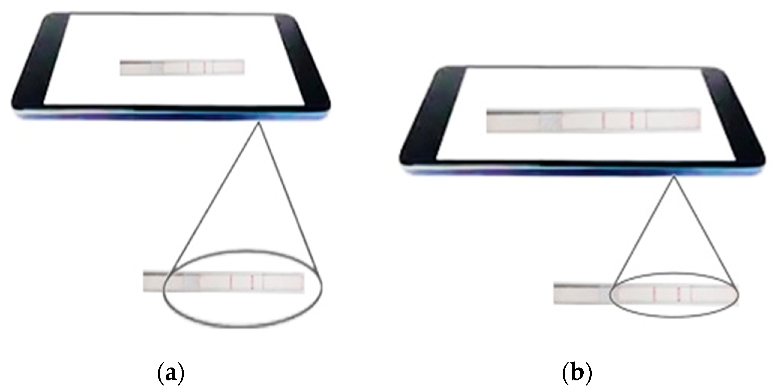
For accurate estimation of the quantity of the analyte, it is essential to detect the ROI precisely. Since mobile devices do not have a fixed position with respect to the test strip, smartphone-based measurement is usually weak and prone to motion blur artifacts [12]. Moreover, due to the inherent unstable nature of the human hand (i.e., movement and shaking) and lack of a stable supporting device (i.e., tripod), the placement of the camera on the exact ROI is difficult, causing the measurement to be erroneous [42]. Hence, for an accurate comparison analysis, the camera must be placed at a certain distance from the test strip covering the ROI for each of the test cases. Figure 13 compares correct (see Figure 13a) and incorrect placements (see Figure 13b) of an LFA strip under a smartphone camera. As shown in Figure 13b, the larger field of view can lead to errors in calculating the number of pixels in the ROI.
In order to counter the challenge of accurate placement, we implemented an additional function in our developed application which helps users to place the strip in a correct position using grids, as shown in Figure 14. Specifically, the application shows a 3 × 3 grid view on the screen and prompts the user to set the control line and test line in a certain position inside the center grid box, as shown in Figure 14b. Thus, the reference distance is fixed for all experiments. To reduce the error due to motion blur artifacts, five readings were taken for each case.
4. Results
The proposed method first approximates the analyte quantities using the regression analysis, and then predicts the quantities using the machine learning classifier, as described in Section 3. Section 4.1 explains the performance metrics to evaluate the regression and classification performance of the proposed method. Then, the regression and classification performance are evaluated in Section 4.2. Section 4.3 shows the smartphone application capability in terms of functionality and efficiency.
4.1. Performance Metrics
The regression analysis of the proposed method shows the relationship between the analyte quantity and the T/C ratio for the acquired readings (mentioned in Section 3.2). The calibration curve, which can be used to approximate the unknown quantity of analyte in the sample, was obtained from the regression analysis. From the curve, the R2 value and the standard error of detection () were calculated according to Equations (4) and (5), respectively.
where SSresidual is the measure of the discrepancy between the data and the estimation model, and SStotal is the sum of the squares of the difference of the obtained data and its mean, and
where Y is an actual data, Y’ is a predicted data, and N is the number of acquired data points. The R2 value shows the statistical measure of proportion of variance, whereas measures the precision of the sample mean of detection. Moreover, the performance of the regression is evaluated in terms of the following metrics: limit of detection (LOD), limit of quantification (LOQ), and coefficient of variation (CV) [43,44]. LOD is the lowest possible concentration of analyte which can be detected with reliability and separated from the limit of blank (LOB). LOB is represented as the maximum quantity of analyte measured when no analyte is present in the sample. LOQ is the lowest quantity of analyte detected with a high confidence level. LOQ is the performance metric for the method or measurement system. CV is the relative variability calculated from the ratio of the standard deviation to the mean. LOD, LOQ, and CV are calculated according to Equations (6)–(8), respectively.
where σ is the standard error of detection, and m is the slope of the calibration curve;
where s is the standard deviation of the readings, and μ is the mean of the readings for each analyte quantity.
On the other hand, the performance of the classifier is evaluated in terms of accuracy, which is defined as follows:
where TP, FP, TN, and FN are the numbers of true positives, false positives, true negatives, and false negatives, respectively.
4.2. Regression and Classification Results
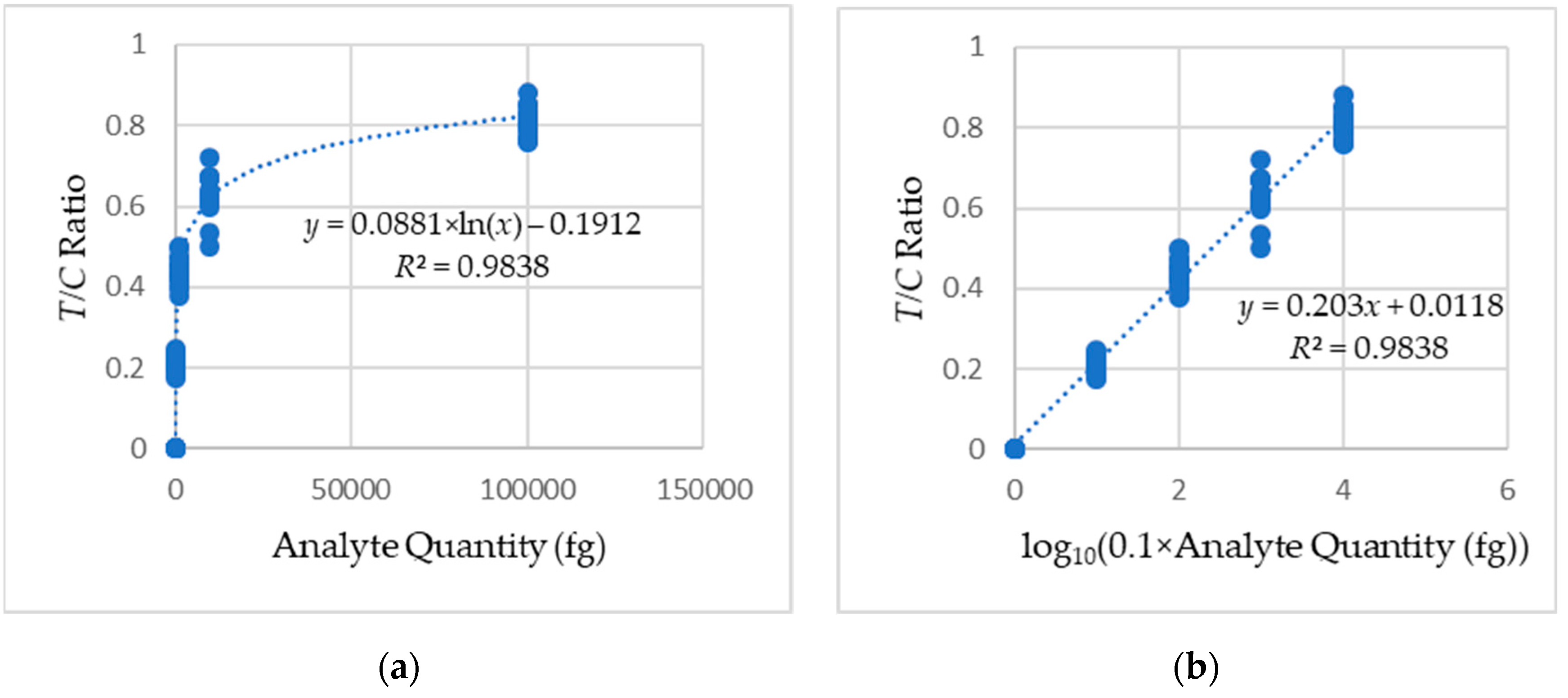
Figure 15 shows the regression analysis of the analyte quantity against T/C ratio. The calibration curve has an equation in the form: y = 0.203x + 0.0118, where x is the analyte quantity, and y is the T/C ratio. The obtained R2 value of 0.9838 from Equation (4) shows a strong correlation between the readings and the fitted calibration curve. The standard error of detection ( value of 0.007 was calculated from Equation (5), and the slope of the calibration curve (m) of 0.203 was obtained from the calibration curve. The limit of detection (LOD) of 0.000026 nM (1.71 pg/mL) and the limit of quantification (LOQ) of 0.00039 nM (26.48 pg/mL) were calculated using the values of and m according to Equations (6) and (7), respectively. The coefficients of variation (CV) obtained from calculations using Equation (8) are shown in Table 4.
A linear SVM classifier with a five-fold cross validation was trained using the approximated quantities obtained from the two training LFA sets. Each set contained the following analyte quantities: 10 fg, 100 fg, 1 pg, 10 pg, and 100 pg. The confusion matrix for the training sets is shown in Table 5. The SVM decision boundary obtained from the training sets was applied to the test LFA set. Each test strip result was evaluated 10 times. The confusion matrix for the testing set is shown in Table 6.
The analyte quantity detection accuracy of the proposed method was calculated to be 98%, according to Equation (9). The performance metrics for the classifier show that our smartphone application could detect four classes out of five with 100% accuracy.
4.3. Smartphone Application Capability
Figure 16 shows the screen captures of five readings of a sample set of LFA strips from our application. The proposed quantitative method was able to detect the analyte quantity instantly after it was trained using the SVM. Training of the proposed method required 0.817 s using a cloud computer equipped with Windows 64-bit, Intel Core i7-6700 CPU @ 3.40 GHz (eight CPUs), 16,384 MB Ram, and MATLAB (2018b) programming.
5. Discussion
Ruppert et al. [45] compared their method to the method used by the ImageJ software [46,47], which is a well-known open platform tool for scientific image analysis. Similarly, we compared our proposed method to the ImageJ software’s method [46,47]. For a fair comparison, Otsu’s thresholding, which is included in our method, was also included in the ImageJ software.
Table 7 compares the performance of the proposed method and the method used by ImageJ software under ambient lighting condition (mentioned in Section 2). The proposed method shows 2.96 times lower LOD and 798.92 times lower LOQ than the ImageJ method, which indicate that the performance of the proposed method was better at quantifying the analyte quantity.
Table 8 compares our proposed method to the conventional methods in terms of functionality. Our method provides a more convenient, portable, robust, and inexpensive solution compared to the existing methods. Moreover, this method has a strong advantage in that only a smartphone is needed to accurately detect the amount of analyte without any additional equipment.
6. Conclusions
In this paper, we have explored the possibility of using a smartphone application to detect the analyte quantity in a sample from an LFA. Using a novel image processing technique and SVM algorithm, we have proposed an automated smartphone application–based method for the detection of analyte quantity in LFA with acceptable accuracy. Our proposed smartphone application can successfully measure the analyte quantity in a sample from a set of LFA strips of analyte quantity varying from 10 fg to 100 pg (1 pg/mL to 10 ng/mL of concentration for 10 uL solution). An overall accuracy of 98.00% in the detection of unknown analyte quantities validated the promising performance of our application, which provides a convenient and rapid LFA reading. Our proposed method also supports the ubiquity (i.e., independent operability under a range of external lighting conditions), portability (i.e., no external device is required), efficiency (i.e., the method can determine the amount of analyte readily), and reliability (i.e., the proposed method achieved a reasonable accuracy in the test case) of our application. It can replace existing methods for the low-cost detection of LFA analytes in different application fields.
Author Contributions
K.H.F. designed the analysis, developed the software, wrote the original and revised manuscript, and conducted data analysis and details of the work. S.E.S. collected the data set, re-designed the research experiment, verified data, and conducted statistical analysis. M.J.K. collected the data and conducted the analysis. O.S.K. conceptualized and designed the research experiment. J.W.C. wrote the original/revised drafts, designed, re-designed, and verified image data analysis, and guided direction of the work.
Funding
This research was supported by a National Research Foundation of Korea (NRF) Grant funded by the Ministry of Science and Information and Communication Technology (ICT) for First-Mover Program for Accelerating Disruptive Technology Development (NRF-2018M3C1B9069834); the National Research Foundation of Korea (NRF) Grant funded by the Ministry of Science and Information and Communication Technology (ICT) (NRF-2019M3C1B8077544); Korea Institute of Planning and Evaluation for Technology in Food, Agriculture and Forestry (IPET) through the Advanced Production Technology Development Program, funded by Ministry of Agriculture, Food and Rural Affairs (MAFRA) (318104-3); the Brain Research Program through the National Research Foundation of Korea (NRF) funded by the Ministry of Science, Information and Communication Technology (ICT) & Future Planning (NRF-2016M3C7A1905384); and the Korea Research Institute of Bioscience and Biotechnology (KRIBB) Initiative Research Program.
Conflicts of Interest
The authors declare no conflict of interest.
References
- Wong, R.C.; Harley, Y.T. Quantitative, false positive, and false negative issues for lateral flow immunoassays as exemplified by onsite drug screens. In Lateral Flow Immunoassay; Humana Press: New York, NY, USA, 2009; pp. 1–19. [Google Scholar]
- Koczula, K.M.; Gallotta, A. Lateral Flow Assays. Essays Biochem. 2016, 60, 111–120. [Google Scholar] [PubMed]
- Pronovost, A.D.; Lee, T.T. Assays and Devices for Distinguishing between Normal and Abnormal Pregnancy. U.S. Patent 5,786,220, 28 July 1998. [Google Scholar]
- Mak, W.C.; Beni, V.; Turner, A.P. Lateral-flow technology: From visual to instrumental. TrAC Trends Anal. Chem. 2016, 79, 297–305. [Google Scholar] [CrossRef]
- Manabe, Y.C.; Nonyane, B.A.S.; Nakiyingi, L.; Mbabazi, O.; Lubega, G.; Shah, M.; Moulton, L.H.; Joloba, M.; Ellner, J.; Dorman, S.E. Point-of-Care Lateral Flow Assays for Tuberculosis and Cryptococcal Antigenuria Predict Death in HIV Infected Adults in Uganda. PLoS ONE 2014, 9, e101459. [Google Scholar] [CrossRef] [PubMed]
- Sun, J.; Xianyu, Y.; Jiang, X. Point-of-care biochemical assays using gold nanoparticle-implemented microfluidics. Chem. Soc. Rev. 2014, 43, 6239–6253. [Google Scholar] [CrossRef] [PubMed]
- Wang, X.; Li, K.; Shi, D.; Xiong, N.; Jin, X.; Yi, J.; Bi, D. Development of an Immunochromatographic Lateral-Flow Test Strip for Rapid Detection of Sulfonamides in Eggs and Chicken Muscles. J. Agric. Food Chem. 2007, 55, 2072–2078. [Google Scholar] [CrossRef]
- Ching, K.H.; He, X.; Stanker, L.H.; Lin, A.V.; McGarvey, J.A.; Hnasko, R. Detection of Shiga Toxins by Lateral Flow Assay. Toxins 2015, 7, 1163–1173. [Google Scholar] [CrossRef] [Green Version]
- Wu, Y.; Xu, M.; Wang, Q.; Zhou, C.; Wang, M.; Zhu, X.; Zhou, D. Recombinase polymerase amplification (RPA) combined with lateral flow (LF) strip for detection of Toxoplasma gondii in the environment. Veter- Parasitol. 2017, 243, 199–203. [Google Scholar] [CrossRef]
- You, M.; Lin, M.; Gong, Y.; Wang, S.; Li, A.; Ji, L.; Zhao, H.; Ling, K.; Wen, T.; Huang, Y.; et al. Household Fluorescent Lateral Flow Strip Platform for Sensitive and Quantitative Prognosis of Heart Failure Using Dual-Color Upconversion Nanoparticles. ACS Nano 2017, 11, 6261–6270. [Google Scholar] [CrossRef]
- Ngom, B.; Guo, Y.; Wang, X.; Bi, D. Development and application of lateral flow test strip technology for detection of infectious agents and chemical contaminants: A review. Anal. Bioanal. Chem. 2010, 397, 1113–1135. [Google Scholar] [CrossRef]
- Carrio, A.; Sampedro, C.; Sánchez-López, J.L.; Pimienta, M.; Campoy, P. Automated Low-Cost Smartphone-Based Lateral Flow Saliva Test Reader for Drugs-of-Abuse Detection. Sensors 2015, 15, 29569–29593. [Google Scholar] [CrossRef] [Green Version]
- Kaylor, R.; Yang, D.; Knotts, M. Reading Device, Method, and System for Conducting Lateral Flow Assays. U.S. Patent 8,367,013, 5 February 2013. [Google Scholar]
- Seo, S.E.; Tabei, F.; Park, S.J.; Askarian, B.; Kim, K.H.; Moallem, G.; Chong, J.W.; Kwon, O.S. Smartphone with optical, physical, and electrochemical nanobiosensors. J. Ind. Eng. Chem. 2019, 77, 1–11. [Google Scholar] [CrossRef]
- Imrich, M.R.; Zeis, J.K.; Miller, S.P.; Pronovost, A.D. Lateral Flow Medical Diagnostic Assay Device with Sample Extraction Means. U.S. Patent 5,415,994, 16 May 1995. [Google Scholar]
- Li, Z.; Chen, H.; Wang, P. Lateral flow assay ruler for quantitative and rapid point-of-care testing. Anal. 2019, 144, 3314–3322. [Google Scholar] [CrossRef] [PubMed]
- Vashist, S.K.; Luppa, P.B.; Yeo, L.Y.; Ozcan, A.; Luong, J.H. Emerging Technologies for Next-Generation Point-of-Care Testing. Trends Biotechnol. 2015, 33, 692–705. [Google Scholar] [CrossRef] [PubMed]
- Zhang, J.-J.; Shen, Z.; Xiang, Y.; Lu, Y. Integration of Solution-Based Assays onto Lateral Flow Device for One-Step Quantitative Point-of-Care Diagnostics Using Personal Glucose Meter. ACS Sensors 2016, 1, 1091–1096. [Google Scholar] [CrossRef]
- You, D.J.; Park, T.S.; Yoon, J.-Y. Cell-phone-based measurement of TSH using Mie scatter optimized lateral flow assays. Biosens. Bioelectron. 2013, 40, 180–185. [Google Scholar] [CrossRef]
- Shen, L.; Hagen, J.A.; Papautsky, I. Point-of-care colorimetric detection with a smartphone. Lab Chip 2012, 12, 4240. [Google Scholar] [CrossRef]
- Cate, D.M.; Adkins, J.A.; Mettakoonpitak, J.; Henry, C.S. Recent Developments in Paper-Based Microfluidic Devices. Anal. Chem. 2014, 87, 19–41. [Google Scholar] [CrossRef]
- Tabei, F.; Zaman, R.; Foysal, K.H.; Kumar, R.; Kim, Y.; Chong, J.W. A novel diversity method for smartphone camera-based heart rhythm signals in the presence of motion and noise artifacts. PLoS ONE 2019, 14, e0218248. [Google Scholar] [CrossRef]
- Srinivasan, B.; O’Dell, D.; Finkelstein, J.L.; Lee, S.; Erickson, D.; Mehta, S. ironPhone: Mobile device-coupled point-of-care diagnostics for assessment of iron status by quantification of serum ferritin. Biosens. Bioelectron. 2018, 99, 115–121. [Google Scholar] [CrossRef]
- Lee, S.; O’Dell, D.; Hohenstein, J.; Colt, S.; Mehta, S.; Erickson, D. NutriPhone: A mobile platform for low-cost point-of-care quantification of vitamin B12 concentrations. Sci. Rep. 2016, 6, 28237. [Google Scholar] [CrossRef]
- Biomedical, D. RDS 2500, Austin, United States. Available online: http://idetekt.com/reader-systems (accessed on 1 August 2019).
- Li, Z.; Wang, Y.; Wang, J.; Tang, Z.; Pounds, J.G.; Lin, Y. Rapid and Sensitive Detection of Protein Biomarker Using a Portable Fluorescence Biosensor Based on Quantum Dots and a Lateral Flow Test Strip. Anal. Chem. 2010, 82, 7008–7014. [Google Scholar] [CrossRef] [PubMed]
- Larsson, K.; Kriz, K.; Kříž, D. Magnetic transducers in biosensors and bioassays. Analusis 1999, 27, 617–621. [Google Scholar] [CrossRef]
- Cooper, D.C.; Callahan, B.; Callahan, P.; Burnett, L. Mobile image ratiometry: A new method for instantaneous analysis of rapid test strips. Nat. Preced. 2012, 10. [Google Scholar] [CrossRef]
- Thieme, T.R.; Cimler, B.M.; Klimkow, N.M. Saliva assay method and device. U.S. Patent 5,714,341, 3 February 1998. [Google Scholar]
- Eltzov, E.; Guttel, S.; Kei, A.L.Y.; Sinawang, P.D.; Ionescu, R.E.; Marks, R.S.; Adarina, L.Y.K.; Ionescu, E.R. Lateral Flow Immunoassays—from Paper Strip to Smartphone Technology. Electroanalysis 2015, 27, 2116–2130. [Google Scholar] [CrossRef]
- O’Farrell, B. Evolution in lateral flow–based immunoassay systems. In Lateral Flow Immunoassay; Humana Press: New York, NY, USA, 2009; pp. 1–33. [Google Scholar]
- Danks, C.; Barker, I. On-site detection of plant pathogens using lateral-flow devices. EPPO Bull. 2000, 30, 421–426. [Google Scholar] [CrossRef]
- Sigma Aldrich, Merck KGaA, Saint Louis, Missouri, USA. Available online: https://www.sigmaaldrich.com/ (accessed on 2 August 2019).
- Samsung Galaxy S7, Samsung Electronics, Ridgefield Park, NJ, USA. Available online: https://www.samsung.com/global/galaxy/galaxy-s7/hardware/ (accessed on 2 August 2019).
- MATLAB 2018b, The Mathworks Inc. Natick, Massachusetts, USA. Available online: https://www.mathworks.com/products/matlab.html (accessed on 2 August 2019).
- Otsu, N. A Threshold Selection Method from Gray-Level Histograms. IEEE Trans. Syst. Man, Cybern. 1979, 9, 62–66. [Google Scholar] [CrossRef] [Green Version]
- Gignac, J.-P. Method of cropping a digital image. U.S. Patent 10/487,995, 2 December 2004. [Google Scholar]
- Priya, M.; Nawaz, D.G.K. Multilevel Image Thresholding using OTSU’s Algorithm in Image Segmentation. Int. J. Sci. Eng. Res. 2017, 8, 101–105. [Google Scholar]
- Zangheri, M.; Di Nardo, F.; Mirasoli, M.; Anfossi, L.; Nascetti, A.; Caputo, D.; De Cesare, G.; Guardigli, M.; Baggiani, C.; Roda, A. Chemiluminescence lateral flow immunoassay cartridge with integrated amorphous silicon photosensors array for human serum albumin detection in urine samples. Anal. Bioanal. Chem. 2016, 408, 8869–8879. [Google Scholar] [CrossRef] [Green Version]
- Lee, S.; Kim, G.; Moon, J. Performance Improvement of the One-Dot Lateral Flow Immunoassay for Aflatoxin B1 by Using a Smartphone-Based Reading System. Sensors 2013, 13, 5109–5116. [Google Scholar] [CrossRef] [Green Version]
- Weston, J.; Watkins, C. Multi-Class Support Vector Machines; Technical Report CSD-TR-98-04; Department of Computer Science, Royal Holloway, University of London: London, UK, May 1998.
- Faulstich, K.; Gruler, R.; Eberhard, M.; Lentzsch, D.; Haberstroh, K. Handheld and portable reader devices for lateral flow immunoassays. In Lateral Flow Immunoassay; Springer: New York, NY, USA, 2009; pp. 1–27. [Google Scholar]
- Armbruster, D.A.; Pry, T. Limit of Blank, Limit of Detection and Limit of Quantitation. Clin. Biochem. Rev. 2008, 29, S49–S52. [Google Scholar]
- Armbruster, D.A.; Tillman, M.D.; Hubbs, L.M. Limit of detection (LQD)/limit of quantitation (LOQ): Comparison of the empirical and the statistical methods exemplified with GC-MS assays of abused drugs. Clin. Chem. 1994, 40, 1233–1238. [Google Scholar] [PubMed]
- Ruppert, C.; Phogat, N.; Laufer, S.; Kohl, M.; Deigner, H.-P. A smartphone readout system for gold nanoparticle-based lateral flow assays: Application to monitoring of digoxigenin. Microchim. Acta 2019, 186, 119. [Google Scholar] [CrossRef] [PubMed]
- ImageJ National Institutes of Health; Bethesda, M.D. USA. Available online: https://imagej.nih.gov/ij/ (accessed on 2 August 2019).
- Abràmoff, M.D.; Magalhães, P.J.; Ram, S.J. Image processing with ImageJ. Biophotonics Int. 2004, 11, 36–42. [Google Scholar]
- Roda, A.; Guardigli, M.; Calabria, D.; Calabretta, M.M.; Cevenini, L.; Michelini, E. A 3D-printed device for a smartphone-based chemiluminescence biosensor for lactate in oral fluid and sweat. Anal. 2014, 139, 6494–6501. [Google Scholar] [CrossRef] [PubMed]
- Mokkapati, V.K.; Sam Niedbala, R.; Kardos, K.; Perez, R.J.; Guo, M.; Tanke, H.J.; Corstjens, P.L. Evaluation of UPlink–RSV: Prototype Rapid Antigen Test for Detection of Respiratory Syncytial Virus Infection. Ann. N. Y. Acad. Sci. 2007, 1098, 476–485. [Google Scholar] [CrossRef] [PubMed]
- Preechaburana, P.; Macken, S.; Suska, A.; Filippini, D. HDR imaging evaluation of a NT-proBNP test with a mobile phone. Biosens. Bioelectron. 2011, 26, 2107–2113. [Google Scholar] [CrossRef]
Figure 1.
Lateral flow assay (LFA) strip architecture where the analyte is detected in the test line, and the red control line indicates that the test was performed.
Figure 1.
Lateral flow assay (LFA) strip architecture where the analyte is detected in the test line, and the red control line indicates that the test was performed.

Figure 2.
(a) Sample LFA strip and (b) region of interest of an LFA strip with an analyte. The intensity and density of red color in the test line region determine the amount of analyte in the sample.
Figure 2.
(a) Sample LFA strip and (b) region of interest of an LFA strip with an analyte. The intensity and density of red color in the test line region determine the amount of analyte in the sample.

Figure 3.
LFA strips for different quantities of analyte under laboratory ambient lighting condition.
Figure 3.
LFA strips for different quantities of analyte under laboratory ambient lighting condition.

Figure 4.
(a) A 3 × 3 grid of the smartphone camera view with proper positioning of LFA, (b) dimension extraction of regions from the center box ((1, 1), (2, 1), (1, 2), (2, 2)), with the test line and the control line position indexes ((0, 1), (3, 1), (0, 2), (3, 2)) and ((0, 2), (3, 2), (0, 3), (3, 3)), respectively, and (c) the control line and the test line regions (marked as A and B, respectively).

Figure 5.
Representation of an image obtained using a Samsung Galaxy S7 smartphone. (a) Alpha-Red-Green-Blue (ARGB) representation of an image. An ARGB image consists of four planes, which are the alpha, red, green, and blue channels. Each channel’s intensity value can vary from 0 to 255. A pixel in the original image shows the combination of the intensity values of the color channels, and (b) the 32-bit representation of a pixel of the image (a). In an ARGB image, each pixel corresponds to a specific 32-bit binary value, of which the lowest eight bits represent blue, the next 8 bits represent green, the next eight bits for red, and the highest eight bits represent the alpha channel intensity values. The pixel’s color is the combination of these color intensities.

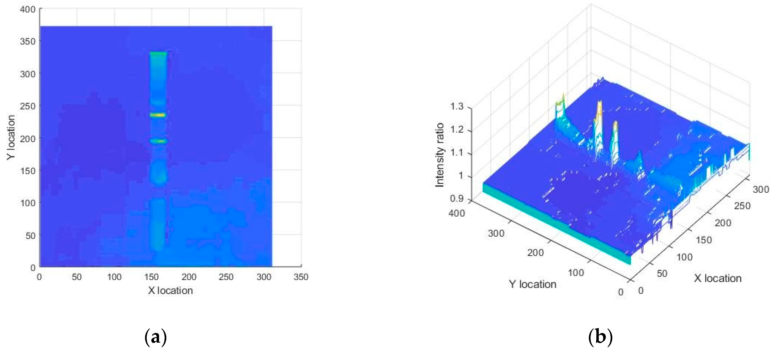
Figure 6.
Ratio of red channel to green channel of a sample LFA strip is visualized by (a) a 2D surface, and (b) a 3D surface. It is clear that the test and control lines had the maximum value that can be used to differentiate them from other regions.
Figure 6.
Ratio of red channel to green channel of a sample LFA strip is visualized by (a) a 2D surface, and (b) a 3D surface. It is clear that the test and control lines had the maximum value that can be used to differentiate them from other regions.

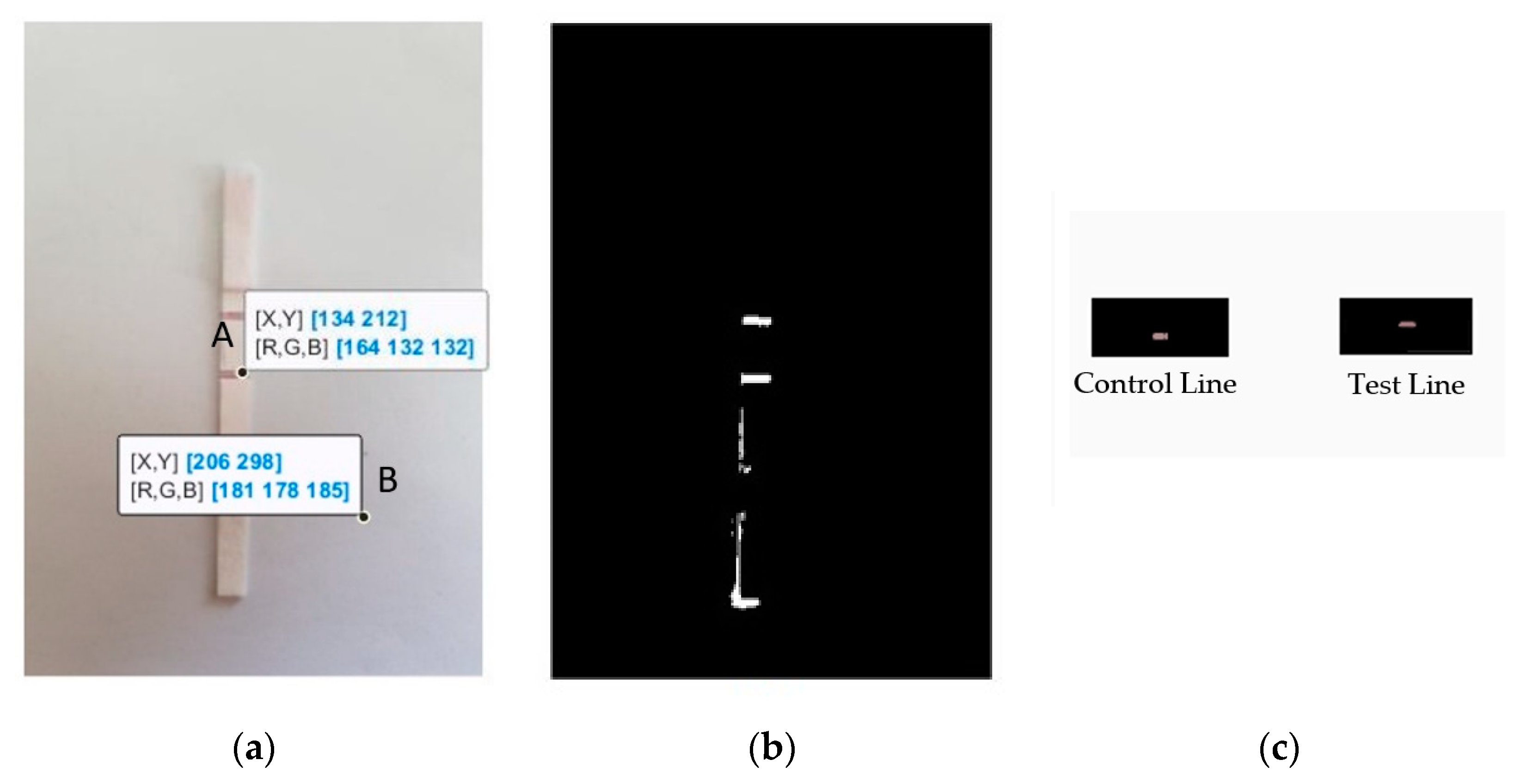
Figure 7.
(a) Visualization of two pixels in a sample LFA strip image with red, green, and blue channel intensity values. Pixel A is in the test line region and pixel B is in the non-ROI region, (b) the calculated mask where the red to green intensity ratio was greater than the threshold THmask, and (c) the extracted control line and test line regions are shown.

Figure 8.
(a) Bar chart for the median of the readings for the weighted sum of the test line red pixels’ intensity values against the quantity of analyte present in the sample in a specific lighting condition; (b) the boxplot for multiple readings for each analyte quantity.
Figure 8.
(a) Bar chart for the median of the readings for the weighted sum of the test line red pixels’ intensity values against the quantity of analyte present in the sample in a specific lighting condition; (b) the boxplot for multiple readings for each analyte quantity.

Figure 9.
LFA strip and calculated T/C ratio for two different lighting conditions: (a) 36-Watt LED ceiling lamp and (b) 27-Watt LED table lamp illuminated environments, showing a similar T/C ratio.
Figure 9.
LFA strip and calculated T/C ratio for two different lighting conditions: (a) 36-Watt LED ceiling lamp and (b) 27-Watt LED table lamp illuminated environments, showing a similar T/C ratio.

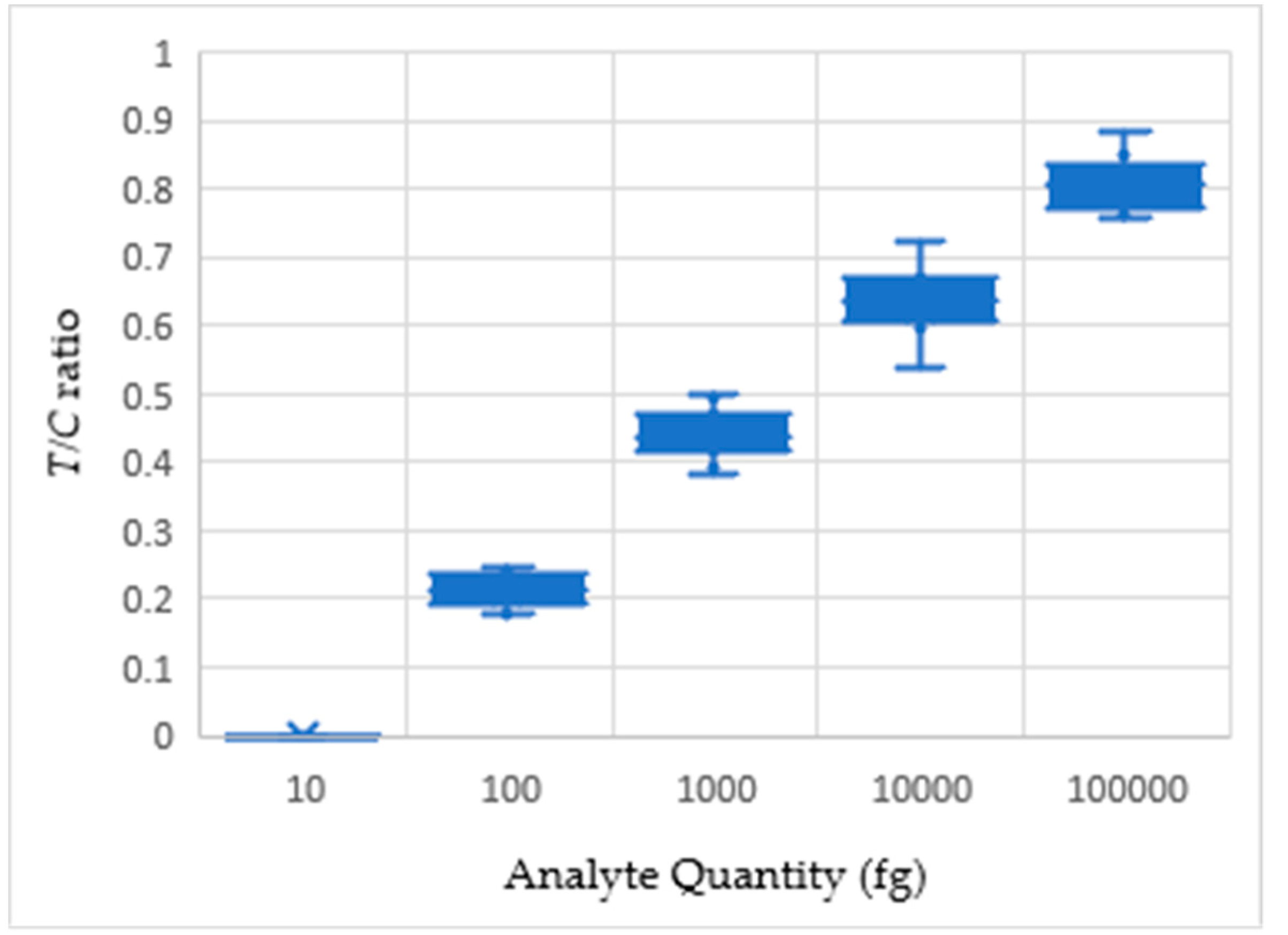
Figure 10.
Analyte quantity against T/C ratio plot for three different LFA sets.

Figure 11.
(a) The flowchart describing the subsequent operations of our developed application; (b) the data acquisition procedure with accurate placement using our developed application.
Figure 11.
(a) The flowchart describing the subsequent operations of our developed application; (b) the data acquisition procedure with accurate placement using our developed application.

Figure 12.
Proposed application for the detection of an analyte in an LFA strip: (a) home screen, (b) second screen with an image capture option, (c) camera view with a 3 × 3 grid spacing, (d) captured raw image, (e) processed image using the created mask (total pixel number shown at the bottom of the image), and (f) calculated control (left) and test (right) line weighted sum of pixels’ intensity values.


Figure 13.
(a) Exact placement of the LFA strip under a smartphone camera and (b) an improper placement of the LFA strip—a larger field of view due to the proximity of the camera to the LFA strip.
Figure 13.
(a) Exact placement of the LFA strip under a smartphone camera and (b) an improper placement of the LFA strip—a larger field of view due to the proximity of the camera to the LFA strip.

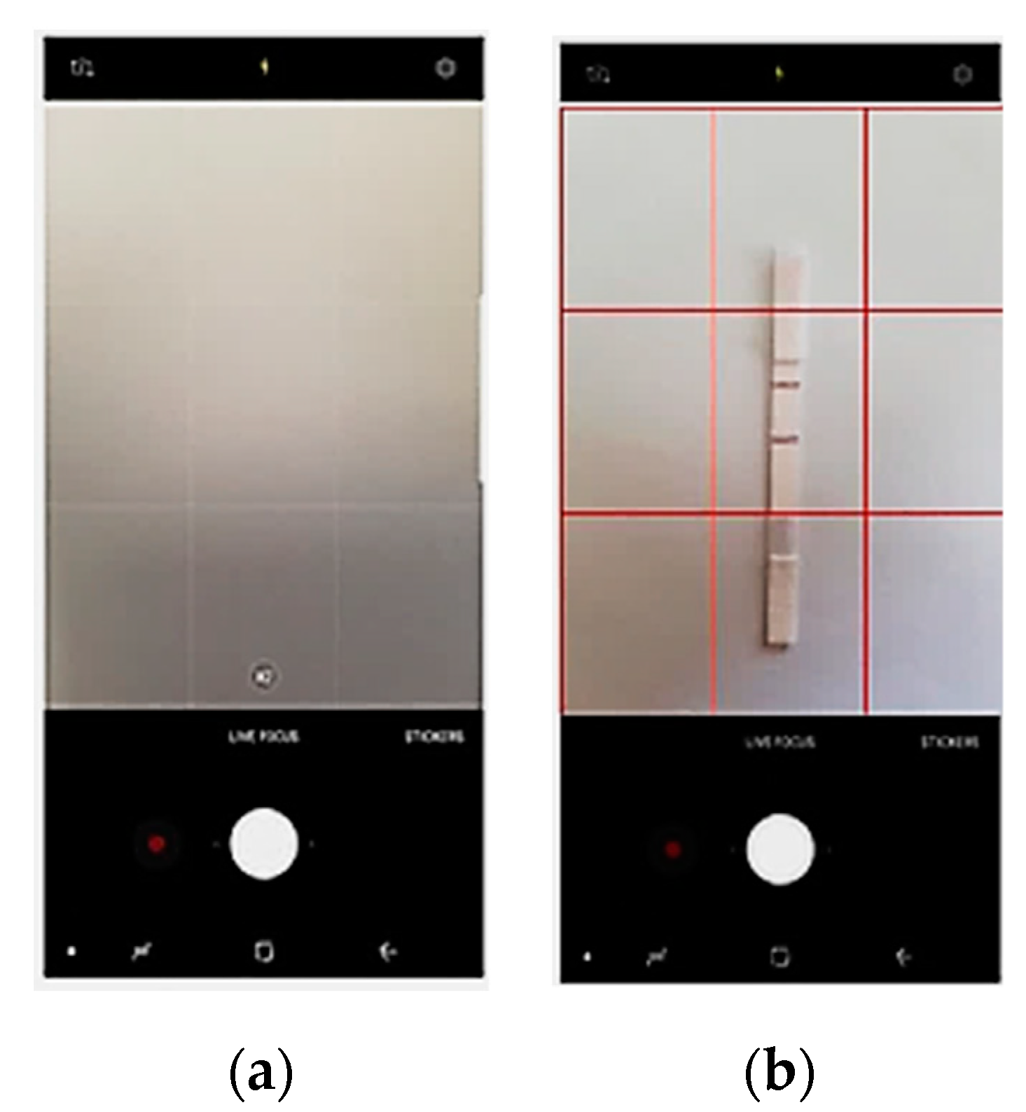
Figure 14.
(a) Android smartphone (Samsung Galaxy) camera view with a 3 × 3 grid positioning and (b) LFA strip ROI positioned in the center box.
Figure 14.
(a) Android smartphone (Samsung Galaxy) camera view with a 3 × 3 grid positioning and (b) LFA strip ROI positioned in the center box.

Figure 15.
Calibration curves obtained from the regression analysis of the LFA sets: (a) logarithmic and (b) linear.
Figure 15.
Calibration curves obtained from the regression analysis of the LFA sets: (a) logarithmic and (b) linear.

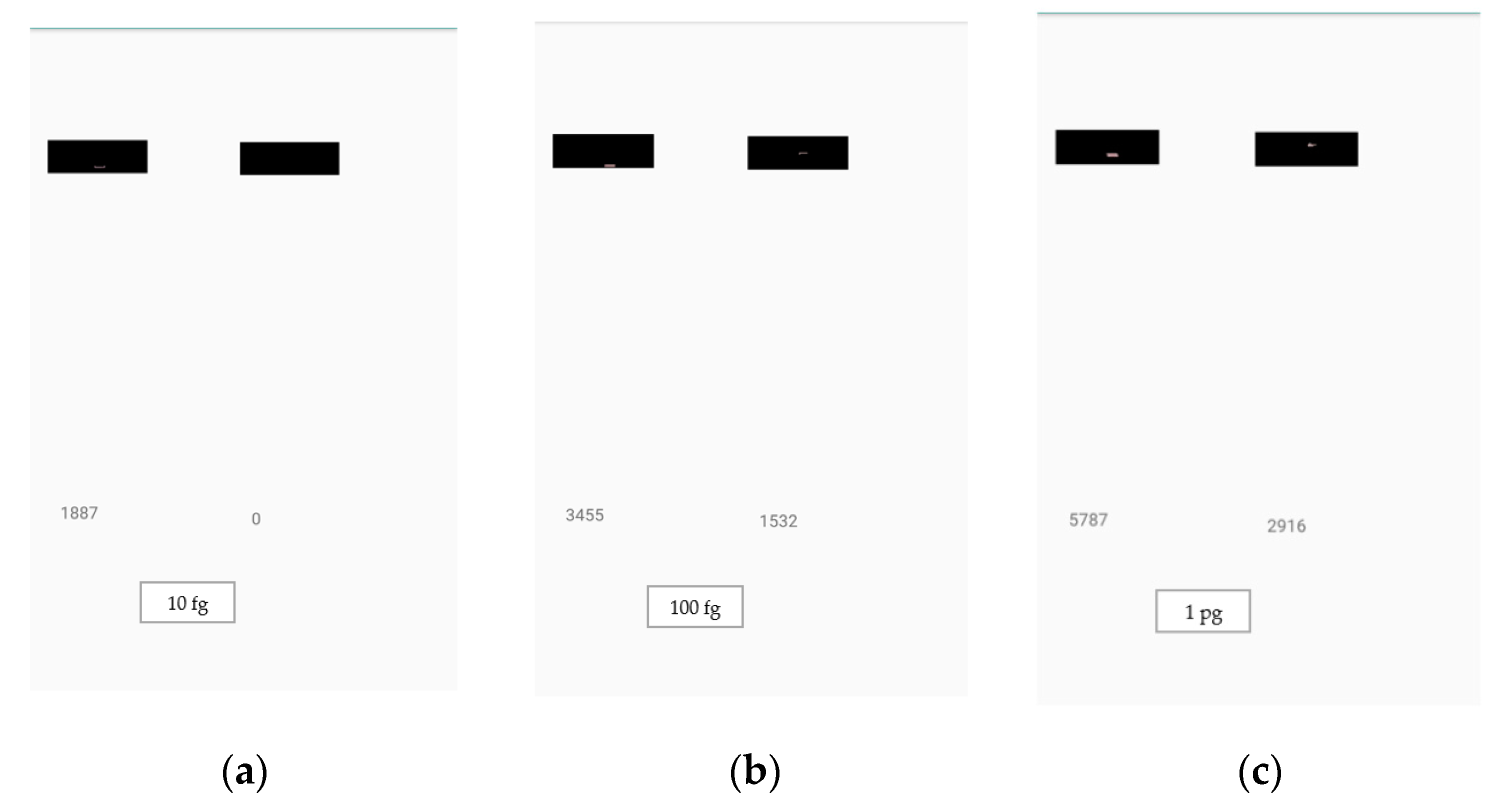
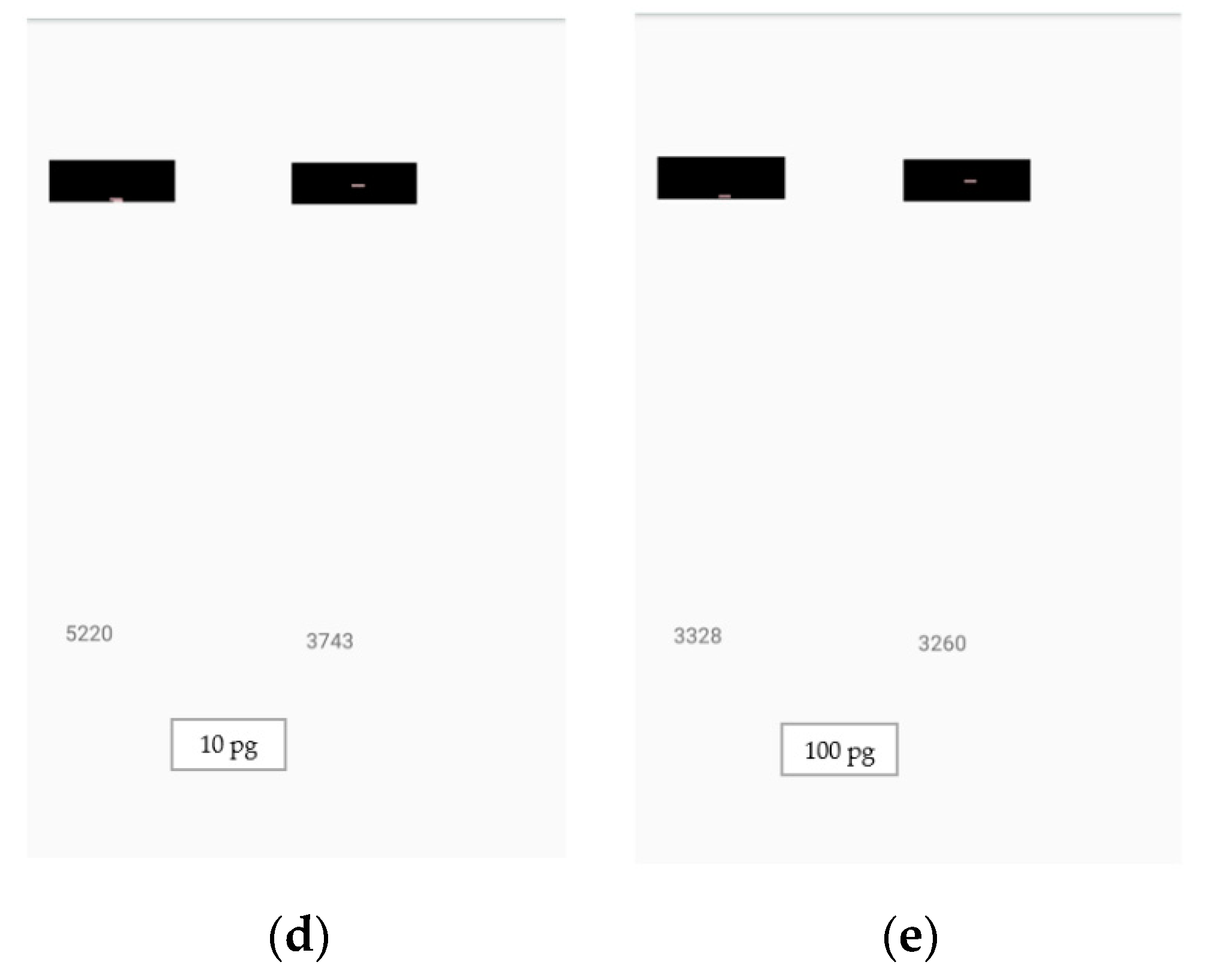
Figure 16.
Estimation of analyte quantity: (a) 10 fg, (b) 100 fg, (c) 1 pg, (d) 10 pg, and (e) 100 pg, using the developed application. The smartphone application was used for the detection of analyte quantities under various lighting conditions. The number on the left is the control line weighted sum of red pixels’ intensities, the number on the right is the test line weighted sum of red pixels’ intensities, and the analyte quantity is displayed at the bottom of the screen.


Table 1.
Calculated T/C ratio for LFA set #1.
| Test Class | Reading 1 | Reading 2 | Reading 3 | Reading 4 | Reading 5 |
|---|---|---|---|---|---|
| 100 pg | 0.764 | 0.782 | 0.772 | 0.758 | 0.762 |
| 10 pg | 0.672 | 0.618 | 0.502 | 0.536 | 0.596 |
| 1 pg | 0.434 | 0.404 | 0.394 | 0.452 | 0.380 |
| 100 fg | 0.21 | 0.234 | 0.20 | 0.18 | 0.194 |
| 10 fg | 0 | 0 | 0 | 0 | 0 |
Table 2.
Calculated T/C ratio for LFA set #2.
| Test Class | Reading 1 | Reading 2 | Reading 3 | Reading 4 | Reading 5 |
|---|---|---|---|---|---|
| 100 pg | 0.806 | 0.807 | 0.82 | 0.85 | 0.836 |
| 10 pg | 0.634 | 0.622 | 0.674 | 0.67 | 0.668 |
| 1 pg | 0.456 | 0.456 | 0.438 | 0.472 | 0.426 |
| 100 fg | 0.246 | 0.242 | 0.212 | 0.226 | 0.176 |
| 10 fg | 0 | 0 | 0 | 0 | 0 |
Table 3.
Calculated T/C ratio for LFA set #3.
| Test Class | Reading 1 | Reading 2 | Reading 3 | Reading 4 | Reading 5 |
|---|---|---|---|---|---|
| 100 pg | 0.796 | 0.828 | 0.882 | 0.64 | 0.798 |
| 10 pg | 0.634 | 0.61 | 0.608 | 0.722 | 0.64 |
| 1 pg | 0.426 | 0.5 | 0.496 | 0.416 | 0.476 |
| 100 fg | 0.238 | 0.204 | 0.208 | 0.194 | 0.22 |
| 10 fg | 0 | 0 | 0 | 0 | 0 |
Table 4.
Mean, std. deviation and coefficient of variation of test to control line signal intensity (T/C) ratios for each of the analyte quantities of the LFA sets.
Table 4.
Mean, std. deviation and coefficient of variation of test to control line signal intensity (T/C) ratios for each of the analyte quantities of the LFA sets.
| Analyte Quantity | Mean T/C Ratio | Std. Deviation of T/C Ratio | CV (%) |
|---|---|---|---|
| 100 pg | 0.791502 | 0.055011 | 6.950253 |
| 10 pg | 0.624684 | 0.055213 | 8.838581 |
| 1 pg | 0.440393 | 0.035544 | 8.070897 |
| 100 fg | 0.211211 | 0.021829 | 10.33506 |
| 10 fg | 0 | 0 | 0 |
Table 5.
Confusion matrix for the training sets obtained by the linear support vector machine (SVM) model. The asterisk sign (*) denotes the misclassified analyte quantity for the training LFA sets.
Table 5.
Confusion matrix for the training sets obtained by the linear support vector machine (SVM) model. The asterisk sign (*) denotes the misclassified analyte quantity for the training LFA sets.
| Predicted Class | |||||
|---|---|---|---|---|---|
| Actual Class | 100 pg | 10 pg | 1 pg | 100 fg | 10 fg |
| 100 pg | 10 | 0 | 0 | 0 | 0 |
| 10 pg | 1 * | 9 | 0 | 0 | 0 |
| 1 pg | 0 | 0 | 10 | 0 | 0 |
| 100 fg | 0 | 0 | 0 | 10 | 0 |
| 10 fg | 0 | 0 | 0 | 0 | 10 |
Table 6.
Confusion matrix for testing the method with the SVM. The asterisk sign (*) denotes the misclassified analyte quantity for the test LFA set.
Table 6.
Confusion matrix for testing the method with the SVM. The asterisk sign (*) denotes the misclassified analyte quantity for the test LFA set.
| Predicted Class | |||||
|---|---|---|---|---|---|
| Actual Class | 100 pg | 10 pg | 1 pg | 100 fg | 10 fg |
| 100 pg | 10 | 0 | 0 | 0 | 0 |
| 10 pg | 1 * | 9 | 0 | 0 | 0 |
| 1 pg | 0 | 0 | 10 | 0 | 0 |
| 100 fg | 0 | 0 | 0 | 10 | 0 |
| 10 fg | 0 | 0 | 0 | 0 | 10 |
Table 7.
Performance comparison between ImageJ software and our proposed method.
| Proposed Method | ImageJ Method | |
|---|---|---|
| LOD | 0.000026 nM (1.71 pg/mL) | 0.000077 nM (5.12 pg/mL) |
| LOQ | 0.00039 nM (26.48 pg/mL) | 0.31158 nM (20,720.4 pg/mL) |
Table 8.
Method comparison between existing methods and the proposed method.
| Ruppert et al. [45], Roda et al. [48], Balaji et al. [23] | Mokkapati et al. [49], RDS 2500 LFA Reader, Detekt Biomedical LLC. [25] | Preechaburana et al. [50] | Proposed Method | |
|---|---|---|---|---|
| Uses smartphone | Yes | No | Yes | Yes |
| Requires external device | Yes | N/A | No | No |
| Works in varying lighting conditions | N/A | N/A | No | Yes |
| Approximates analyte quantity | Yes | Yes | Yes | Yes |
| Predicts based on machine learning | No | No | No | Yes |
© 2019 by the authors. Licensee MDPI, Basel, Switzerland. This article is an open access article distributed under the terms and conditions of the Creative Commons Attribution (CC BY) license (http://creativecommons.org/licenses/by/4.0/).
Share and Cite
MDPI and ACS Style
Foysal, K.H.; Seo, S.E.; Kim, M.J.; Kwon, O.S.; Chong, J.W. Analyte Quantity Detection from Lateral Flow Assay Using a Smartphone. Sensors 2019, 19, 4812. https://0-doi-org.brum.beds.ac.uk/10.3390/s19214812
AMA Style
Foysal KH, Seo SE, Kim MJ, Kwon OS, Chong JW. Analyte Quantity Detection from Lateral Flow Assay Using a Smartphone. Sensors. 2019; 19(21):4812. https://0-doi-org.brum.beds.ac.uk/10.3390/s19214812
Chicago/Turabian StyleFoysal, Kamrul H., Sung Eun Seo, Min Ju Kim, Oh Seok Kwon, and Jo Woon Chong. 2019. "Analyte Quantity Detection from Lateral Flow Assay Using a Smartphone" Sensors 19, no. 21: 4812. https://0-doi-org.brum.beds.ac.uk/10.3390/s19214812
Note that from the first issue of 2016, this journal uses article numbers instead of page numbers. See further details here.