3D Contact Position Estimation of Image-Based Areal Soft Tactile Sensor with Printed Array Markers and Image Sensors

 ,
,
Abstract
:1. Introduction
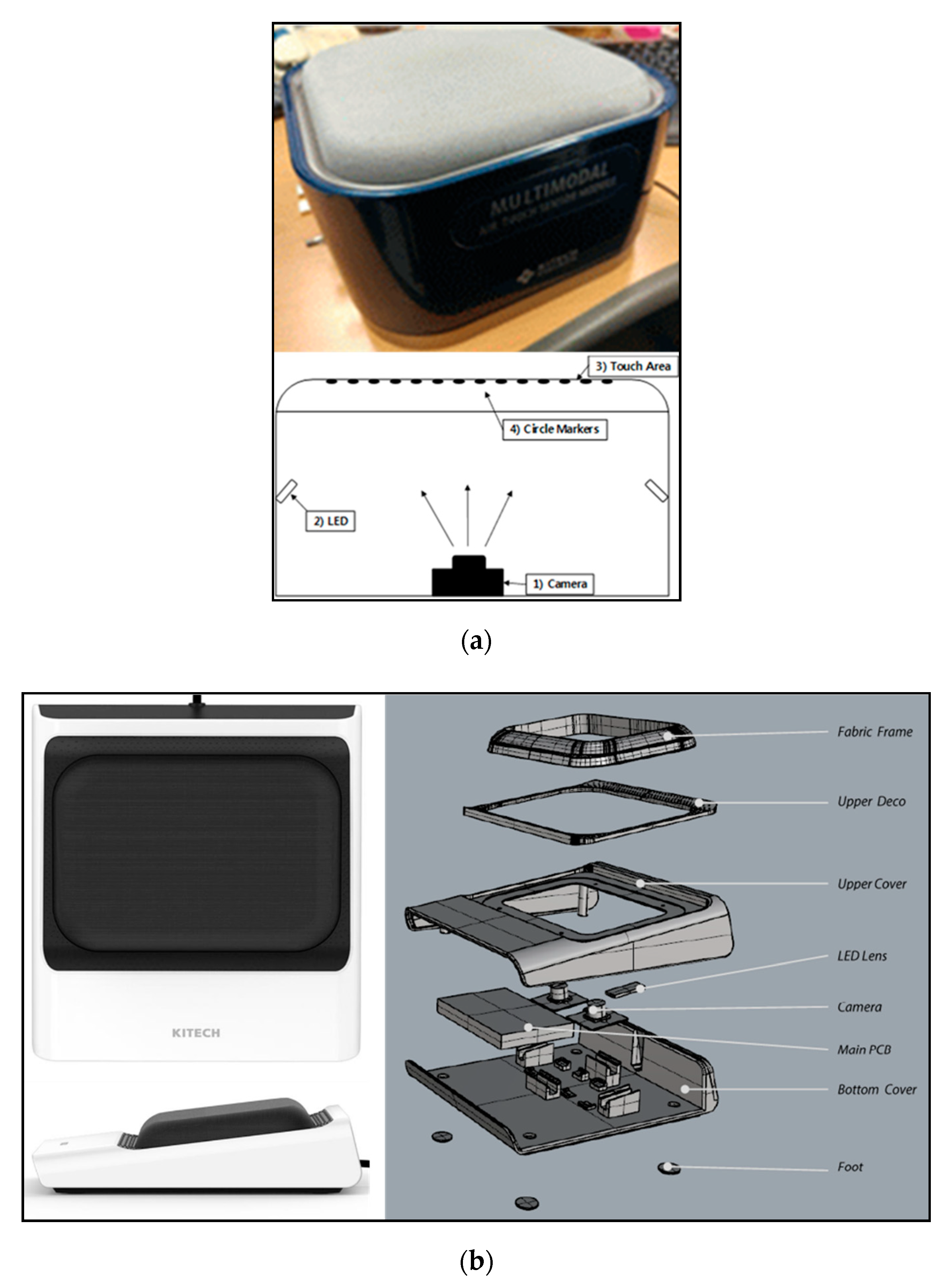
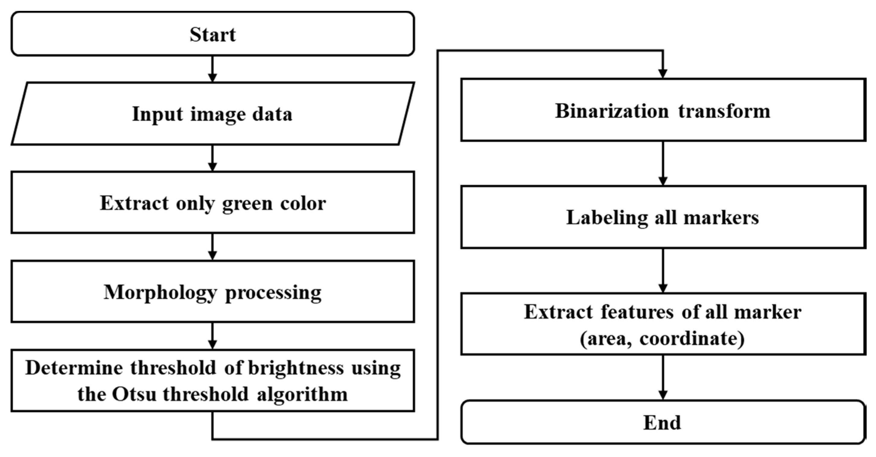
2. Materials and Methods
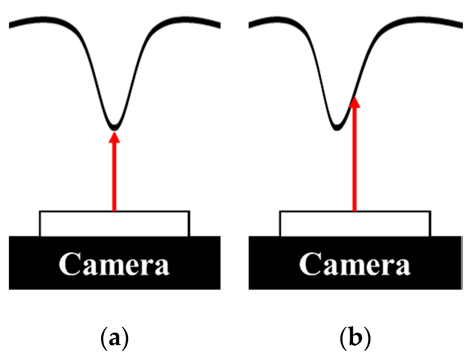
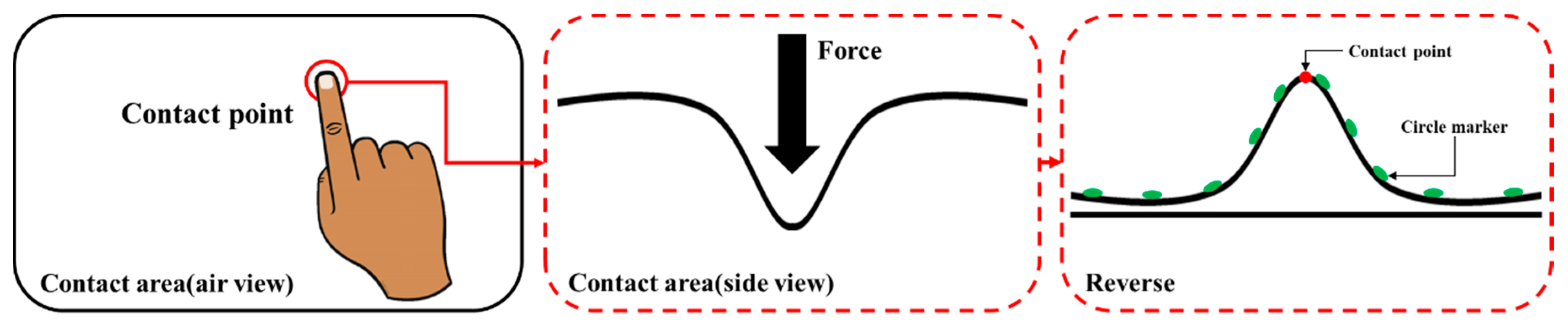
2.1. Contact Position and Depth Estimation Algorithm
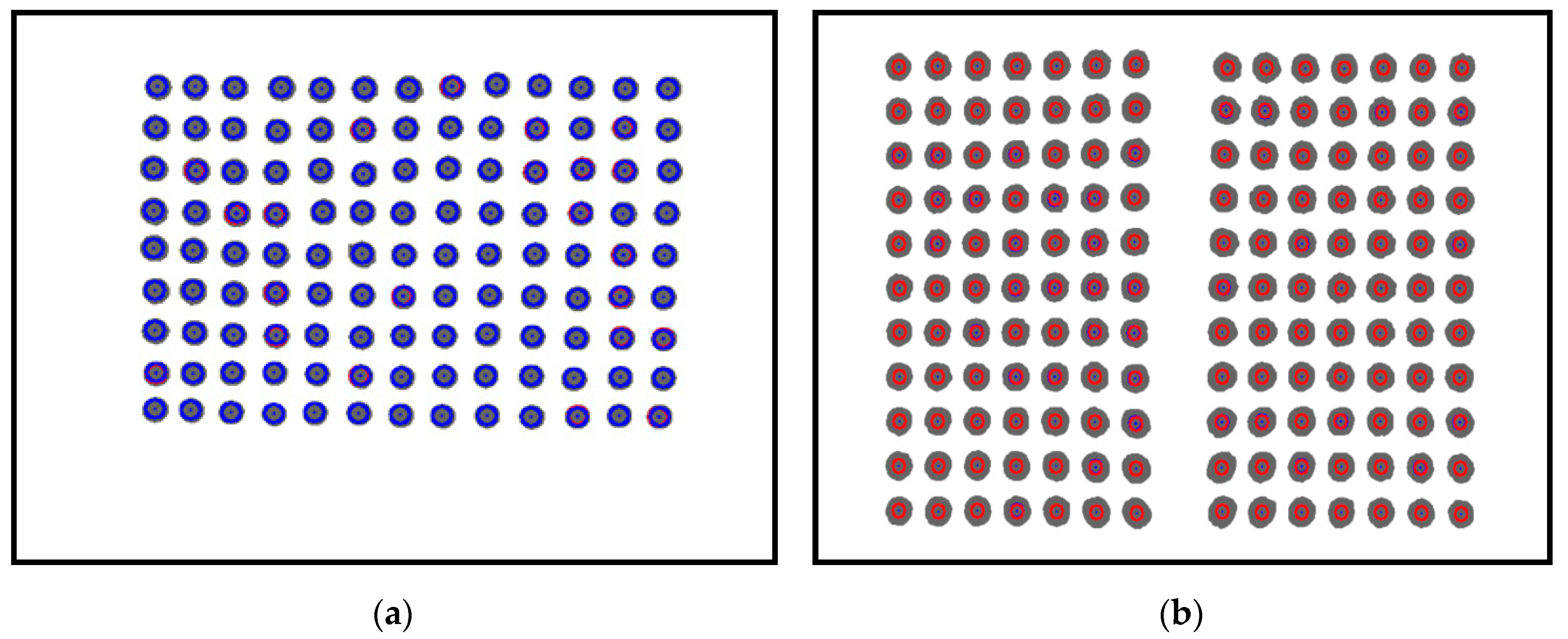
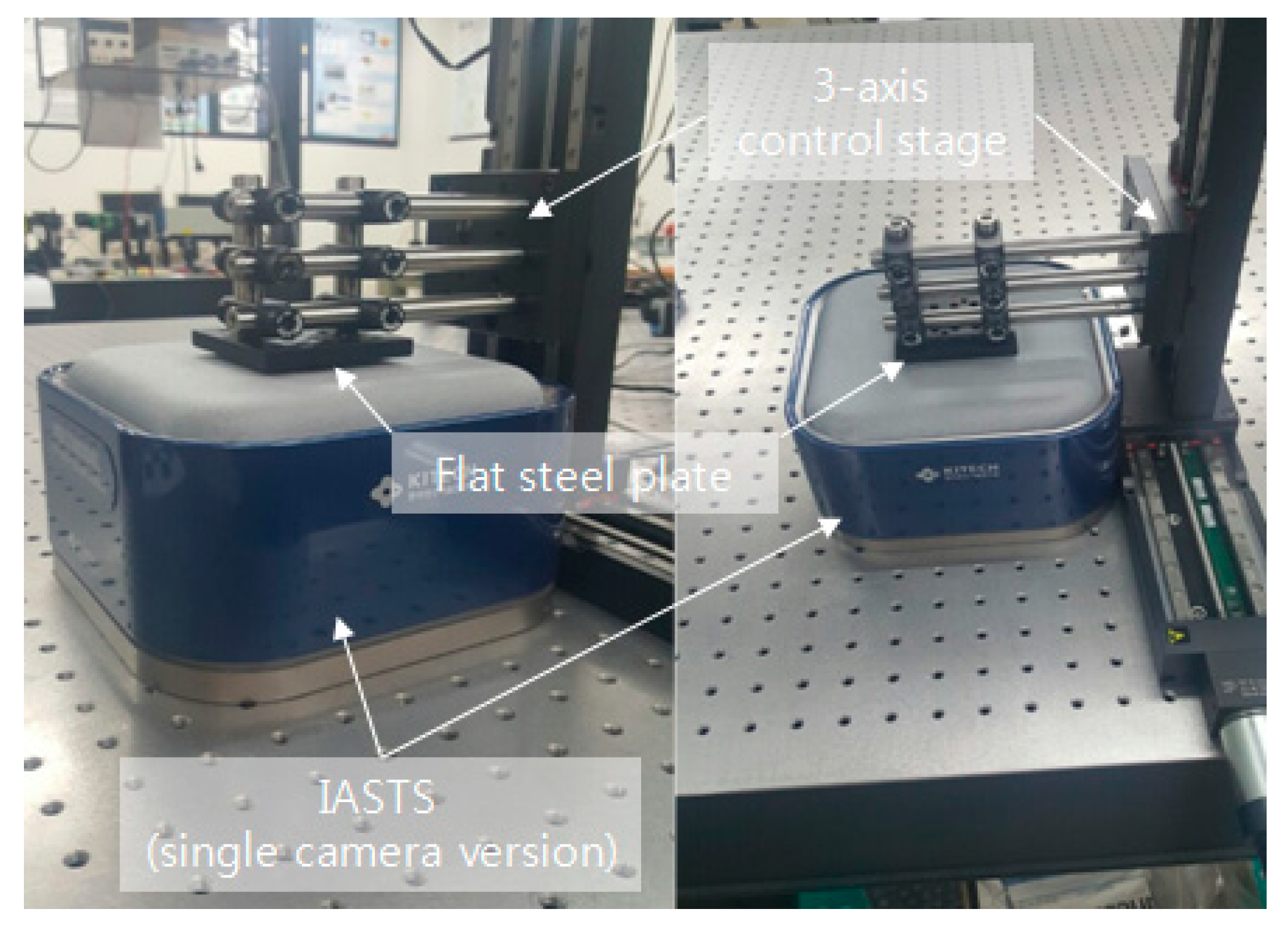
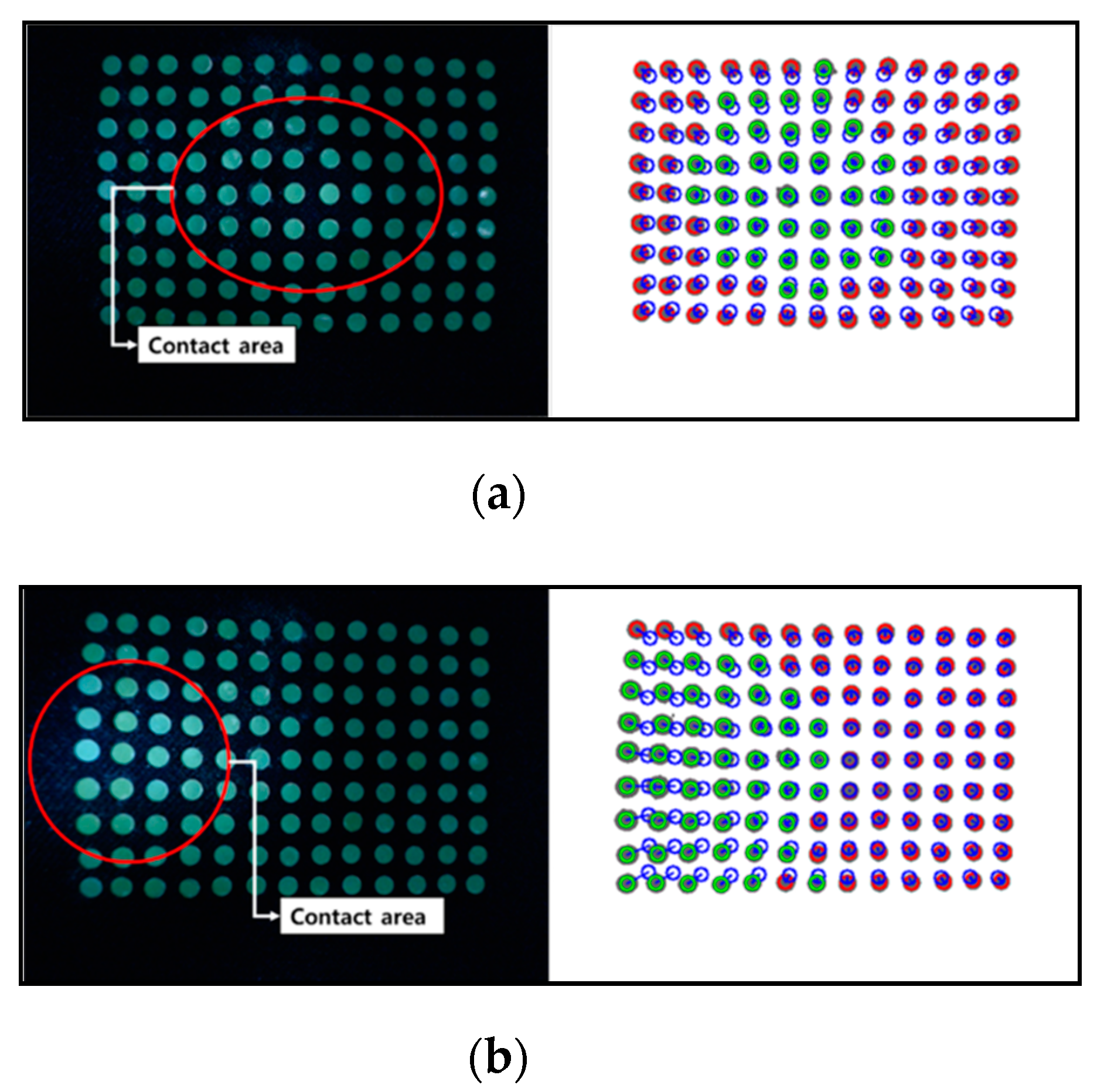
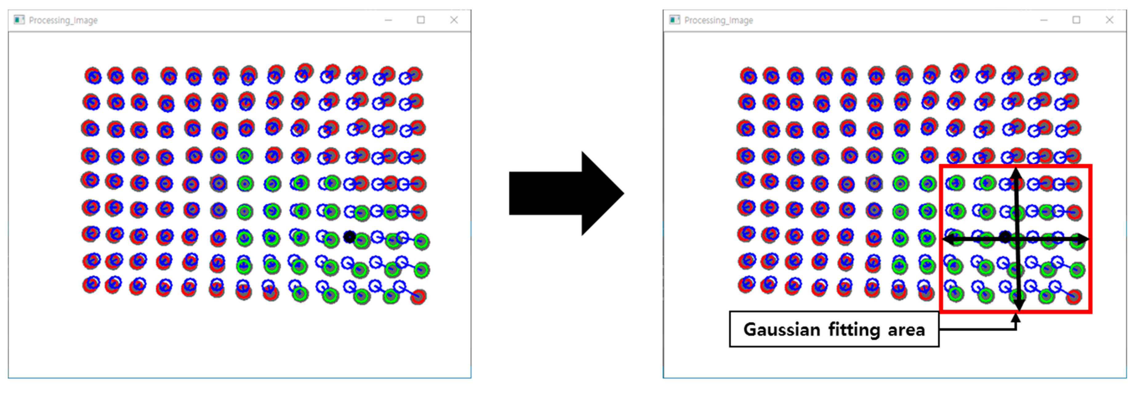
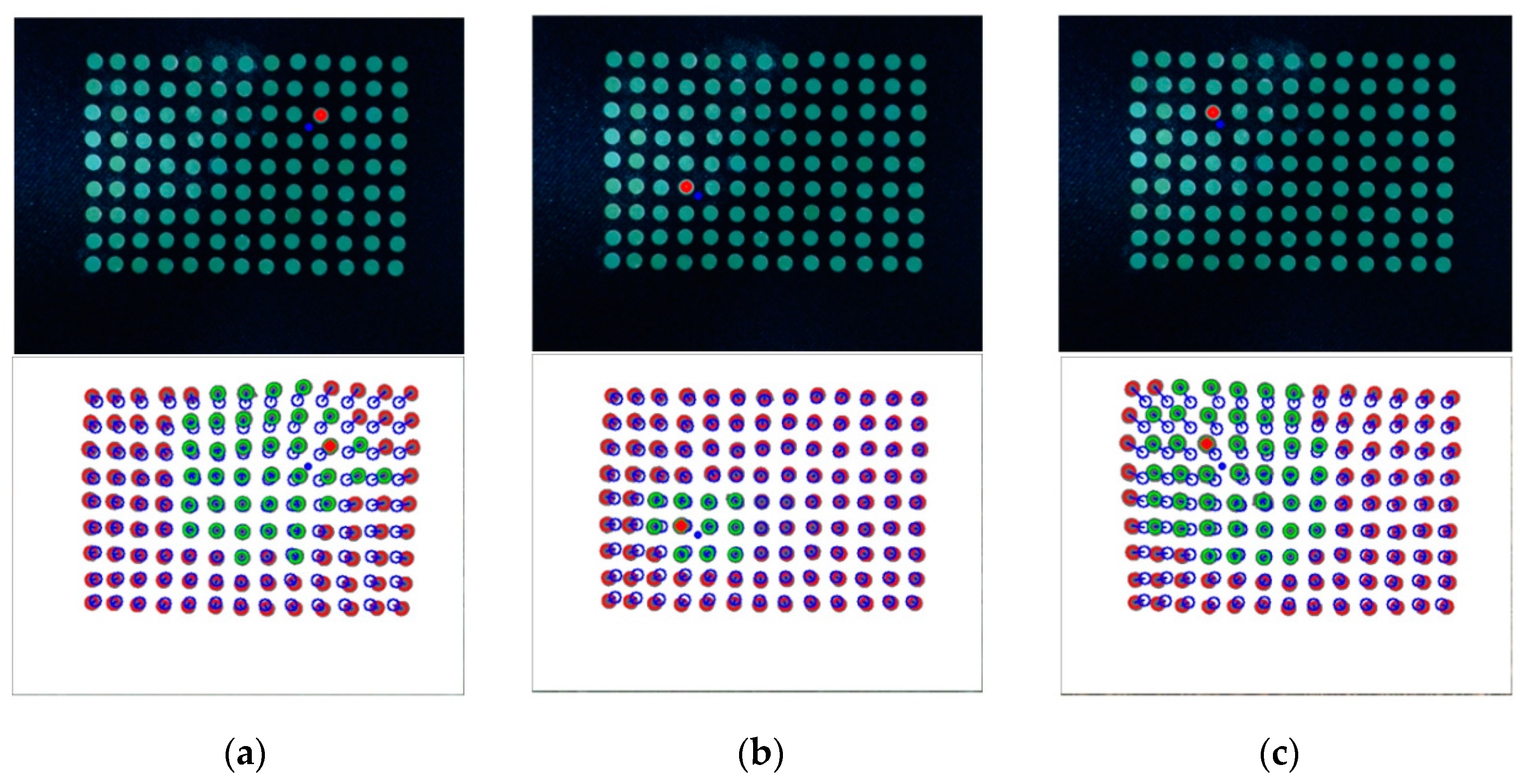
2.2. Image Processing and Feature Extraction
2.3. The Polynomial Fitting Algorithm
2.4. The Gaussian Curve Fitting Algorithm
3. Results
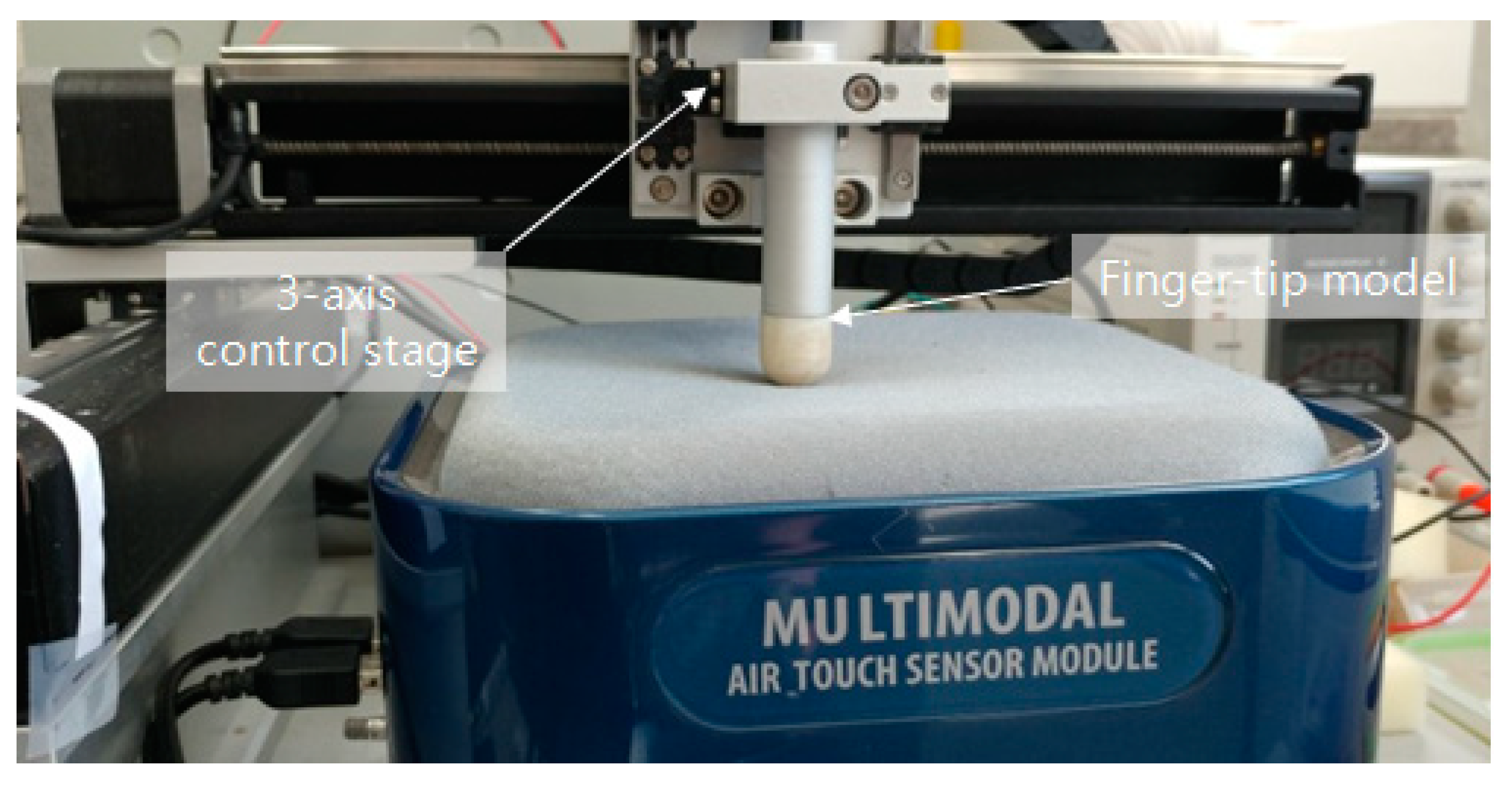
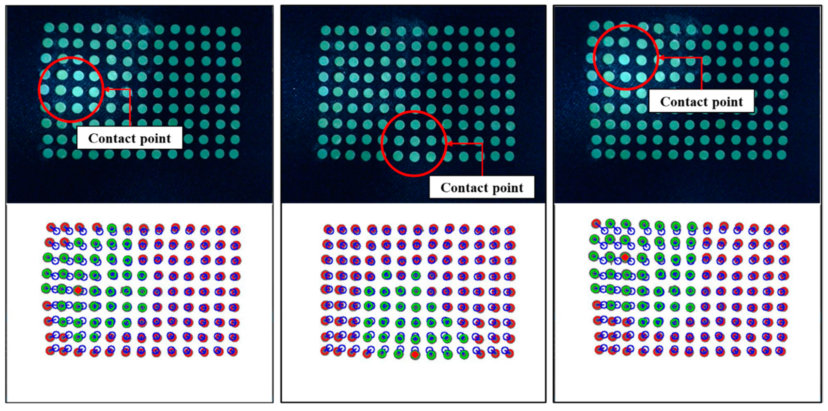
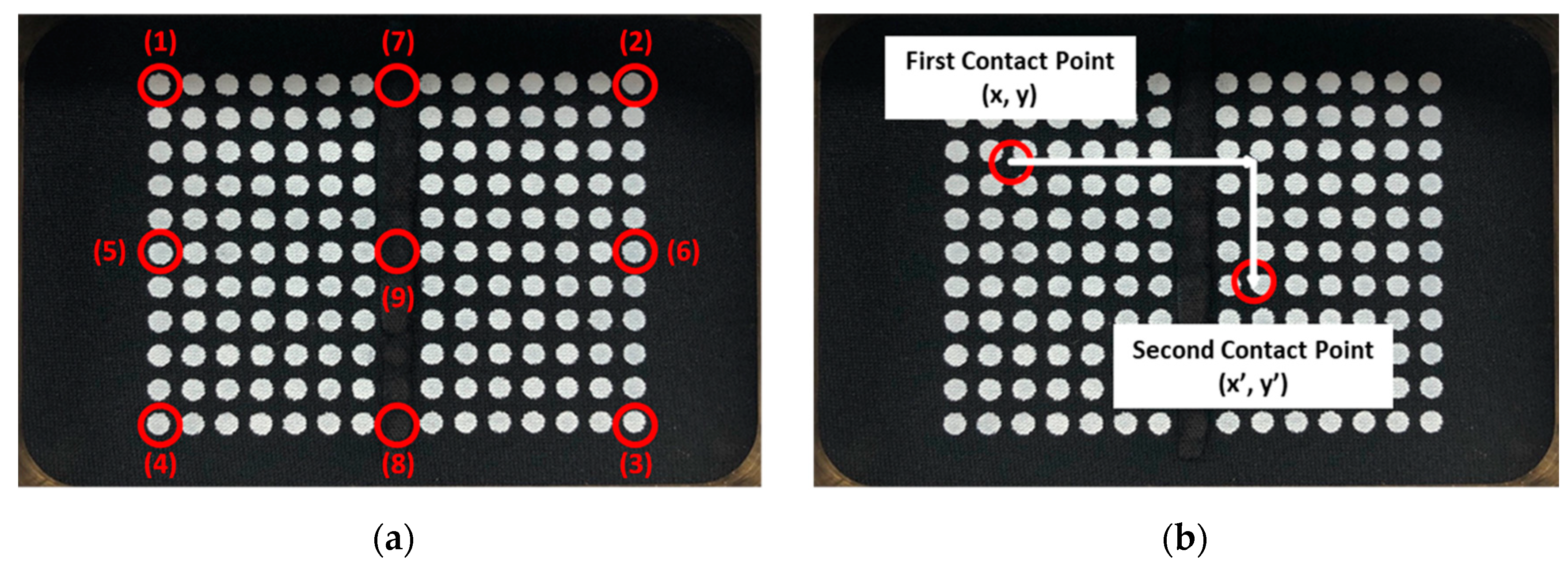
3.1. Experiment of IASTS (Single-Camera Model)
3.2. Experiment of IASTS (Dual-Camera Model)
4. Discussion
5. Conclusions
Author Contributions
Funding
Conflicts of Interest
References
- Sánchez-Durán, J.A.; Hidalgo-López, J.A.; Castellanos-Ramos, J.; Oballe-Peinado, Ó.; Vidal-Verdú, F. Influence of Errors in Tactile Sensors on Some High Level Parameters Used for Manipulation with Robotic Hands. Sensors 2015, 15, 20409–20435. [Google Scholar] [CrossRef] [PubMed] [Green Version]
- Aggarwal, A.; Kirchner, F. Object Recognition and Localization: The Role of Tactile Sensors. Sensors 2014, 14, 3227–3266. [Google Scholar] [CrossRef] [PubMed] [Green Version]
- Kampmann, P.; Kirchner, F. Integration of Fiber-Optic Sensor Arrays into a Multi-Modal Tactile Sensor Processing System for Robotic End-Effectors. Sensors 2014, 14, 6854–6876. [Google Scholar] [CrossRef] [PubMed]
- Kim, Y.; Obinata, G.; Kawk, B.; Jung, J.; Lee, S. Vision-based Fluid-Type Tactile Sensor for Measurements on Biological Tissues. Med. Biol. Eng. Comput. 2018, 56, 297–305. [Google Scholar] [CrossRef] [PubMed]
- Lee, J.H.; Nyun Kim, Y.N.; Park, H.J. Bio-Optics Based Sensation Imaging for Breast Tumor Detection Using Tissue Characterization. Sensors 2015, 15, 6306–6323. [Google Scholar] [CrossRef] [PubMed] [Green Version]
- Jimenez, M.C.; Fishel, J.A. Evaluation of force, vibration and thermal tactile feedback in prosthetic limbs. In Proceedings of the 2014 IEEE Haptics Symposium (HAPTICS), Houston, TX, USA, 23–26 February 2014. [Google Scholar]
- Muxfeldt, A.; Haus, N.; Cheng, A.; Kubus, J.D. Exploring tactile surface sensors as a gesture input device for intuitive robot programming. In Proceedings of the 2016 IEEE 21st International Conference on Emerging Technologies and Factory Automation (ETFA), Berlin, Germany, 6–9 September 2016. [Google Scholar]
- Pradhono, T.; Somlor, S.; Schmitz, A.; Jamone, L.; Huang, W.; Kristanto, H.; Sugano, S. Design and Characterization of a Three-Axis Hall Effect-Based Soft Skin Sensor. Sensors 2016, 16, 491. [Google Scholar] [CrossRef] [PubMed]
- Alves de Oliveira, T.E.; Cretu, A.M.; Petriu, E.M. Multimodal Bio-Inspired Tactile Sensing Module for Surface Characterization. Sensors 2017, 17, 1187. [Google Scholar] [CrossRef] [PubMed] [Green Version]
- Maiolino, P.; Maggiali, M.; Cannata, G.; Metta, G.; Natale, L. A Flexible and Robust Large Scale Capacitive Tactile System for Robots, Friction, and Stiffness. IEEE Sens. J. 2013, 13, 3910–3917. [Google Scholar] [CrossRef]
- Lamy, X.; Colledani, F.; Geffard, F.; Measson, Y.; Morel, G. Robotic skin structure and performances for industrial robot comanipulation. In Proceedings of the IEEE/ASME International Conference on Advanced Intelligent Mechatronics, Singapore, 14–17 July 2009. [Google Scholar]
- Cirrillo, A.; Cirrillo, P.; Maria, G.D.; Natale, C.; Pirozzi, S. Improved Version of the Tactile/Force Sensor Based on Optoelectronic Technology. Procedia Eng. 2016, 168, 826–829. [Google Scholar] [CrossRef]
- Melchiorri, C.; Moriello, L.; Palli, G.; Scarcia, U. A new force/torque sensor for robotic application based on optoelectronic components. In Proceedings of the International Conference on Robotics and Automation (ICRA2014), Hong Kong, China, 31 May–7 June 2014. [Google Scholar]
- Missinne, J.; Bosman, E.; Van Hoe, B.; Van Steenberge, G.; Kalathimekkad, S.; Van Daele, P.; Vanfleteren, J. Flexible Shear Sensor Based on Embedded Optoelectronic Components. IEEE Photon. Technol. Lett. 2011, 23, 771–773. [Google Scholar] [CrossRef]
- Fishel, J.; Loeb, G. Sensing tactile microvibrations with the BioTac—Comparison with human sensitivity. In Proceedings of the IEEE International Conference on Biomedical Robotics and Biomechatronics, Rome, Italy, 24–27 June 2012. [Google Scholar]
- Su, Z.; Fishel, J.; Yamamoto, T.; Loeb, G. Use of Tactile Feedback to Control Exploratory Movements to Characterize Object Compliance. Front. Neurorobot. 2012, 6, 1–9. [Google Scholar]
- Sferrazza, C.; Wahlsten, A.; Trueeb, C.; Andrea, R.D. Ground Truth Force Distribution for Learning-Based Tactile Sensing: A Finite Element Approach. IEEE Access 2019, 7, 173438–173449. [Google Scholar] [CrossRef]
- Trueeb, C.; Sferrazza, C.; Andrea, R.D. Towards vision-based robotic skins: A data-driven, multi-camera tactile sensor. arXiv 2019, arXiv:1910.14526. [Google Scholar]
- Lee, J.; Cho, B.; Choi, S.; Kwon, S.; Kim, M.; Lee, S. Image-based 3-axis force estimation of a touch sensor with soft material. In Proceedings of the 2016 16th International Conference on Control, Automation and Systems (ICCAS 2016), Gyeongju, Korea, 16–19 October 2016. [Google Scholar]
- Lee, J.; Lee, S.; Cho, B.; Kwon, K.; Oh, H.; Kim, M. Contact Position Estimation Algorithm using Image-based Areal Touch Sensor based on Artificial Neural Network. IEEJ J. Ind. Appl. 2018, 6, 100. [Google Scholar] [CrossRef]
- Sato, K.; Kamiyama, K.; Nii, H.; Kawakami, N.; Tachi, S. Measurement of force vector field of robotic finger using vision-based haptic sensor. In Proceedings of the IEEE/RSJ International Conference on Intelligent Robots and Systems (IROS 2008), Nice, France, 22–26 September 2008. [Google Scholar]
- Sato, K.; Kamiyama, K.; Kawakami, N.; Tachi, S. Finger-Shaped GelForce: Sensor for Measuring Surface Traction Fields for Robotic Hand. IEEE Trans. Haptics. 2010, 3, 37–47. [Google Scholar] [CrossRef] [PubMed]
- Yamaguchi, A.; Atkeson, C. Combining finger vision and optical tactile sensing: Reducing and handling errors while cutting vegetables. In Proceedings of the 2016 IEEE-RAS 16th International Conference on Humanoid Robots (Humanoids 2016), Cancun, Mexico, 15–17 November 2016. [Google Scholar]
- Ito, Y.; Kim, Y.; Obinata, G. Robust Slippage Degree Estimation Based on Reference Update of Vision-Based Tactile Sensor. IEEE Sens. J. 2011, 11, 2037–2047. [Google Scholar] [CrossRef]
- Ito, Y.; Kim, Y.; Nagai, C.; Obinata, G. Shape sensing by vision-based tactile sensor for dexterous handling of robot hands. In Proceedings of the 2010 IEEE International Conference on Automation Science and Engineering, 2010 (CASE2010), Toronto, Canada, 21–24 August 2010. [Google Scholar]
- Lepora, N. Biomimetic Active Touch with Fingertips and Whiskers. IEEE Trans. Haptics 2016, 9, 170–183. [Google Scholar] [CrossRef] [PubMed] [Green Version]
- Cramphorn, L.; Ward-Cherrier, B.; Lepora, N. Addition of a Biomimetic Fingerprint on an Artificial Fingertip Enhances Tactile Spatial Acuity. IEEE Robot. Autom. Lett. 2017, 2, 1336–1343. [Google Scholar] [CrossRef] [PubMed] [Green Version]


| Experiment | Real Contact | Estimated Contact | Error Distance | Real Depth Value | Estimated Depth Value | Error Depth | |||
|---|---|---|---|---|---|---|---|---|---|
| X | Y | X | Y | X | Y | ||||
| (a) | 43 | 13 | 43.14 | 14.29 | 0.14 | 1.29 | 10 | 10.76 | 0.76 |
| 42.66 | 14.12 | 0.34 | 1.12 | 10.79 | 0.79 | ||||
| 42.35 | 14.44 | 0.65 | 1.44 | 10.65 | 0.65 | ||||
| (b) | 14 | 28 | 16.54 | 30.11 | 2.54 | 2.11 | 7 | 7.2 | 0.2 |
| 16.75 | 29.95 | 2.75 | 1.95 | 7.15 | 0.15 | ||||
| 16.41 | 29.84 | 2.41 | 1.84 | 7.15 | 0.15 | ||||
| (c) | 16 | 11 | 15.41 | 14.31 | 0.59 | 3.31 | 13 | 14.52 | 1.52 |
| 15.36 | 14.22 | 0.64 | 3.22 | 14.81 | 1.81 | ||||
| 15.52 | 14.33 | 0.48 | 3.33 | 14.52 | 1.52 | ||||
| Experiment | Real Contact | Estimated Contact | Error Distance | Error Rate (%) | ||||
|---|---|---|---|---|---|---|---|---|
| X | Y | X | Y | X | Y | X | Y | |
| 1 | 107 | 70 | 104 | 76 | 3 | 6 | 2.80 | 8.57 |
| 2 | 841 | 70 | 846 | 77 | 5 | 7 | 0.59 | 10.00 |
| 3 | 841 | 580 | 846 | 590 | 5 | 10 | 0.59 | 1.72 |
| 4 | 107 | 580 | 115 | 590 | 8 | 10 | 7.48 | 1.72 |
| 5 | 107 | 325 | 116 | 322 | 9 | 3 | 8.41 | 0.92 |
| 6 | 842 | 325 | 845 | 321 | 3 | 4 | 0.36 | 1.23 |
| 7 | 475 | 70 | 480 | 79 | 5 | 9 | 1.05 | 12.86 |
| 8 | 475 | 580 | 467 | 590 | 8 | 10 | 1.68 | 1.72 |
| 9 | 475 | 325 | 479 | 320 | 4 | 5 | 0.84 | 1.54 |
| Experiment | Real Depth | Estimated Depth | Error Depth | Error Rate (%) |
|---|---|---|---|---|
| 1 | 1.00 | 0.89 | 0.11 | 11.00 |
| 2.00 | 1.91 | 0.09 | 4.50 | |
| 3.00 | 2.89 | 0.11 | 3.67 | |
| 2 | 1.00 | 0.85 | 0.15 | 15.00 |
| 2.00 | 1.89 | 0.11 | 5.50 | |
| 3.00 | 2.92 | 0.08 | 2.67 | |
| 3 | 1.00 | 1.09 | 0.09 | 9.00 |
| 2.00 | 2.11 | 0.11 | 5.50 | |
| 3.00 | 3.13 | 0.13 | 4.33 | |
| 4 | 1.00 | 1.07 | 0.07 | 7.00 |
| 2.00 | 2.08 | 0.08 | 4.00 | |
| 3.00 | 3.08 | 0.08 | 2.67 | |
| 5 | 1.00 | 1.03 | 0.03 | 3.00 |
| 2.00 | 2.01 | 0.01 | 0.50 | |
| 3.00 | 2.98 | 0.02 | 0.67 | |
| 6 | 1.00 | 1.06 | 0.06 | 6.00 |
| 2.00 | 1.98 | 0.02 | 1.00 | |
| 3.00 | 2.97 | 0.03 | 1.00 | |
| 7 | 1.00 | 1.05 | 0.05 | 5.00 |
| 2.00 | 2.04 | 0.04 | 2.00 | |
| 3.00 | 3.01 | 0.01 | 0.33 | |
| 8 | 1.00 | 1.03 | 0.03 | 3.00 |
| 2.00 | 2.02 | 0.02 | 1.00 | |
| 3.00 | 3.04 | 0.04 | 1.33 | |
| 9 | 1.00 | 0.98 | 0.02 | 2.00 |
| 2.00 | 1.97 | 0.03 | 1.50 | |
| 3.00 | 2.99 | 0.01 | 0.33 |
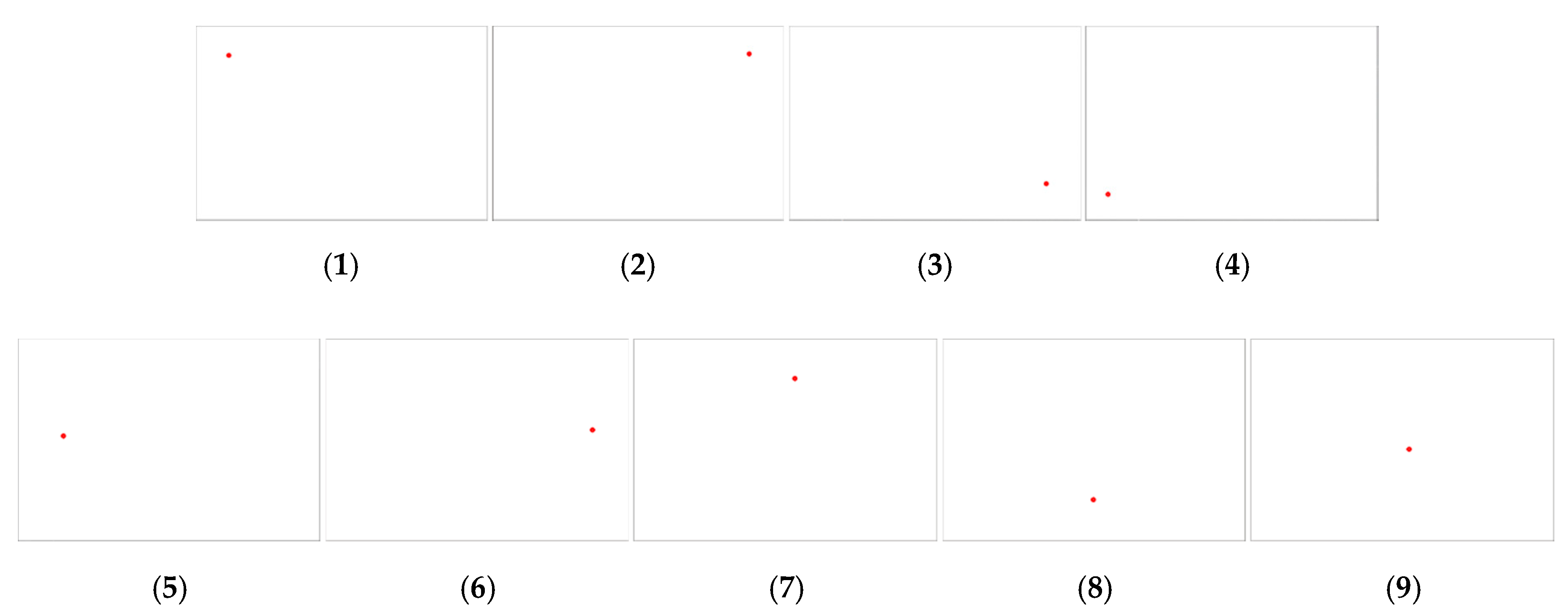
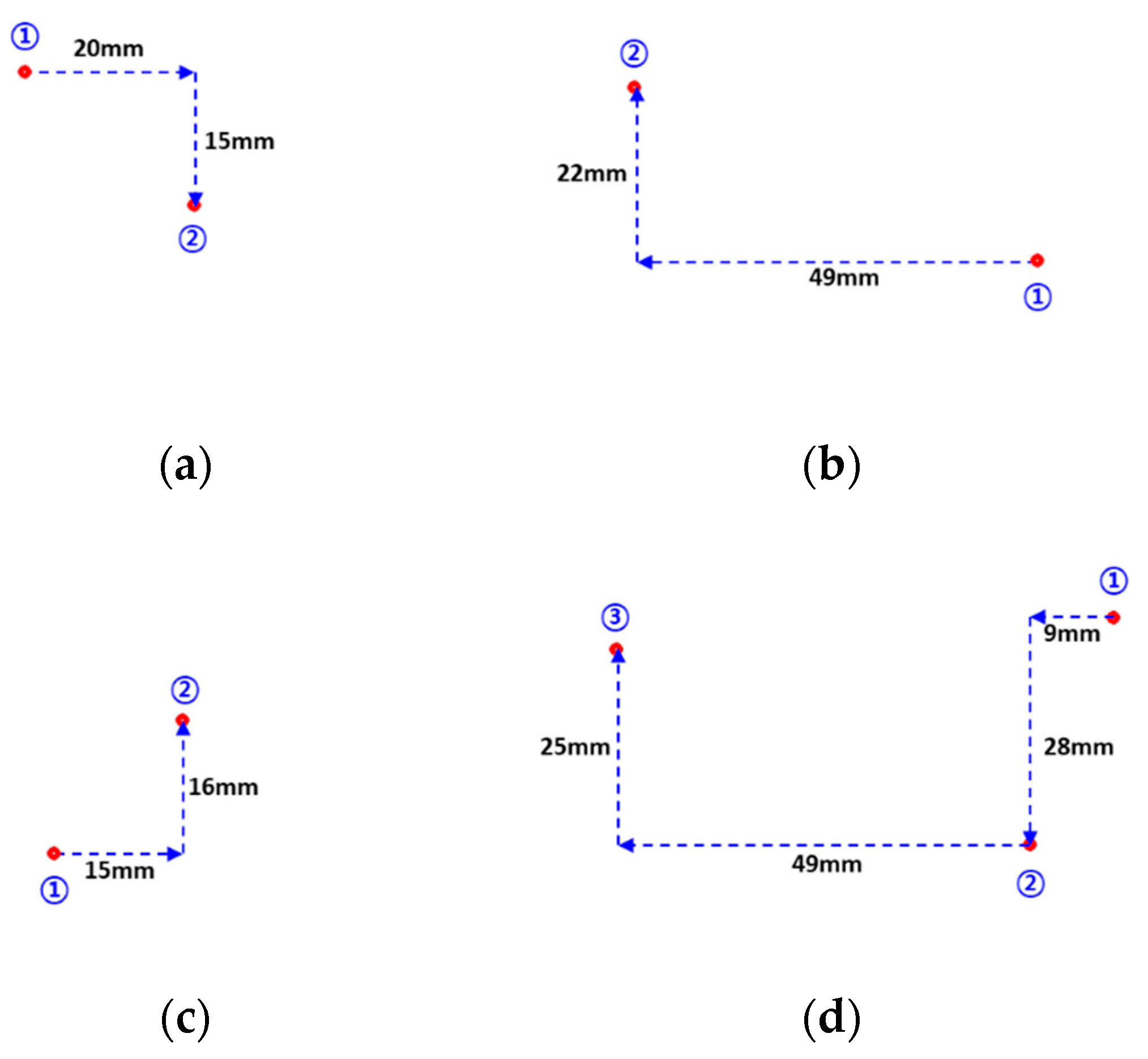
| Experiment | 1st Contact Position (Pixel) | 2nd Contact Position (Pixel) | Moving Distance (mm) | Coordinate per 1 mm | |
|---|---|---|---|---|---|
| (a) | X | 259 | 466 | +20 mm | 10.35 |
| Y | 215 | 377 | +15 mm | 10.80 | |
| (b) | X | 712 | 220 | −49 mm | 10.04 |
| Y | 420 | 210 | −22 mm | 9.55 | |
| (c) | X | 305 | 466 | +15 mm | 10.73 |
| Y | 503 | 341 | −16 mm | 10.13 | |
| (d_1) | X | 845 | 744 | −9 mm | 11.22 |
| Y | 181 | 460 | +28 mm | 10.37 | |
| (d_2) | X | 744 | 236 | −49 mm | 9.96 |
| Y | 460 | 219 | −25 mm | 9.64 | |
© 2020 by the authors. Licensee MDPI, Basel, Switzerland. This article is an open access article distributed under the terms and conditions of the Creative Commons Attribution (CC BY) license (http://creativecommons.org/licenses/by/4.0/).
Share and Cite
Lee, J.-i.; Lee, S.; Oh, H.-M.; Cho, B.R.; Seo, K.-H.; Kim, M.Y. 3D Contact Position Estimation of Image-Based Areal Soft Tactile Sensor with Printed Array Markers and Image Sensors. Sensors 2020, 20, 3796. https://0-doi-org.brum.beds.ac.uk/10.3390/s20133796
Lee J-i, Lee S, Oh H-M, Cho BR, Seo K-H, Kim MY. 3D Contact Position Estimation of Image-Based Areal Soft Tactile Sensor with Printed Array Markers and Image Sensors. Sensors. 2020; 20(13):3796. https://0-doi-org.brum.beds.ac.uk/10.3390/s20133796
Chicago/Turabian StyleLee, Jong-il, Suwoong Lee, Hyun-Min Oh, Bo Ram Cho, Kap-Ho Seo, and Min Young Kim. 2020. "3D Contact Position Estimation of Image-Based Areal Soft Tactile Sensor with Printed Array Markers and Image Sensors" Sensors 20, no. 13: 3796. https://0-doi-org.brum.beds.ac.uk/10.3390/s20133796