A Self-Powered Wireless Water Quality Sensing Network Enabling Smart Monitoring of Biological and Chemical Stability in Supply Systems

 , , ,
, , , 
Abstract
:1. Introduction
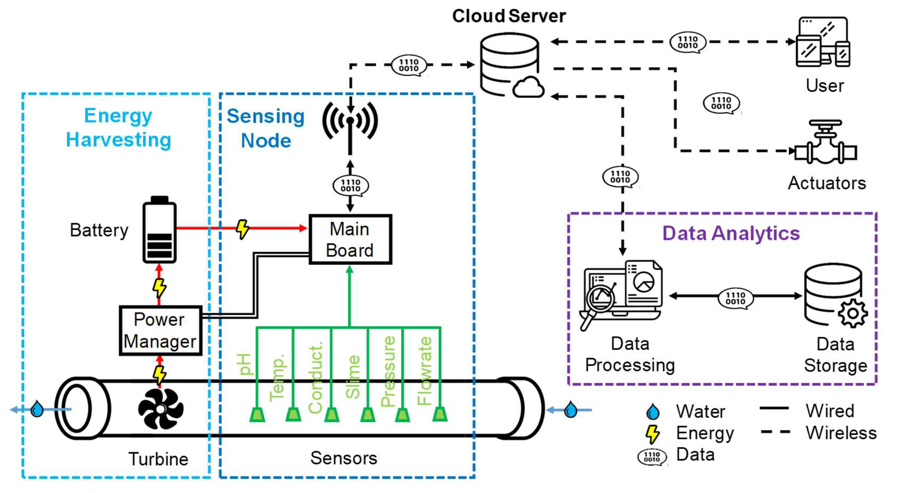
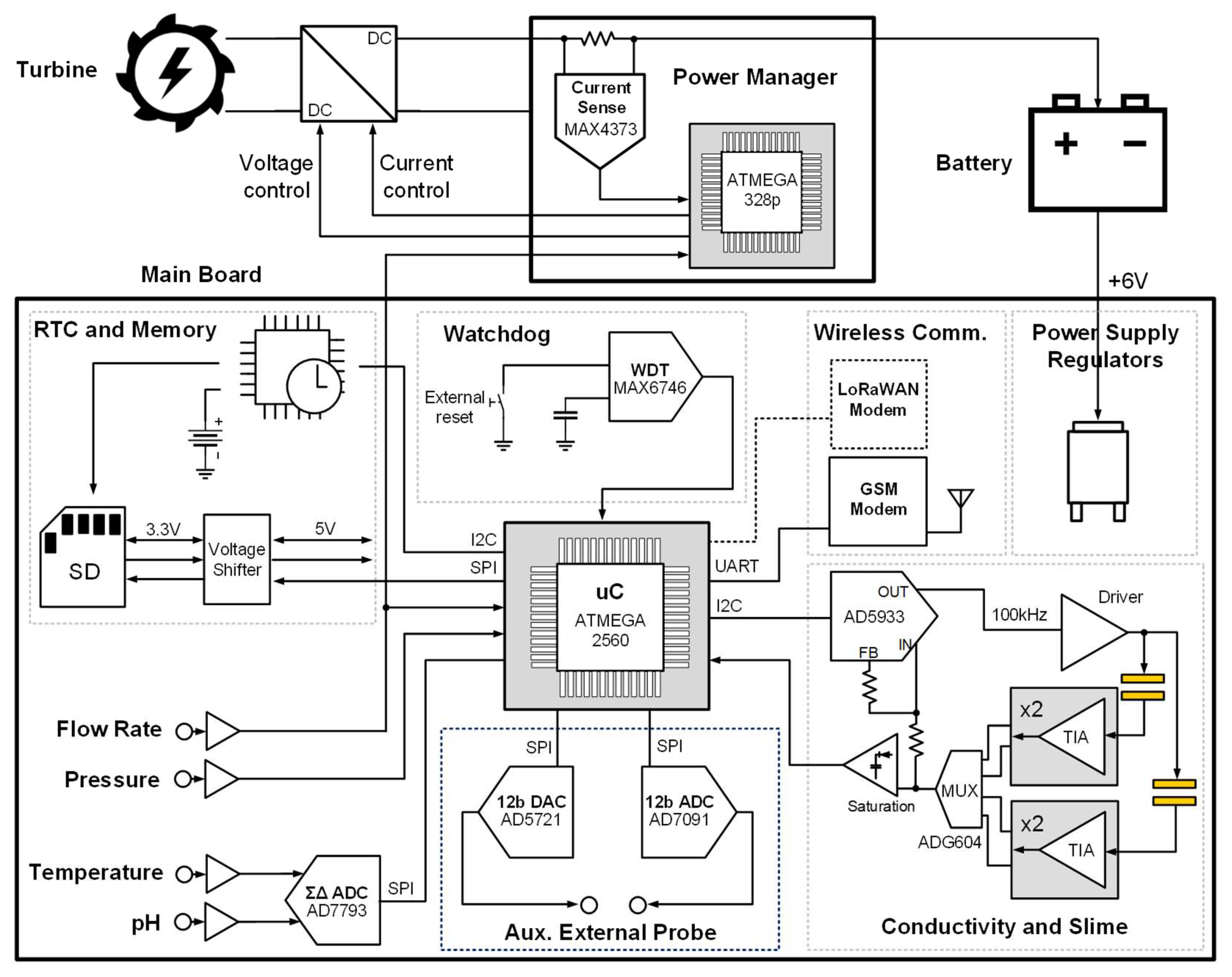
2. System Architecture
3. Sensors
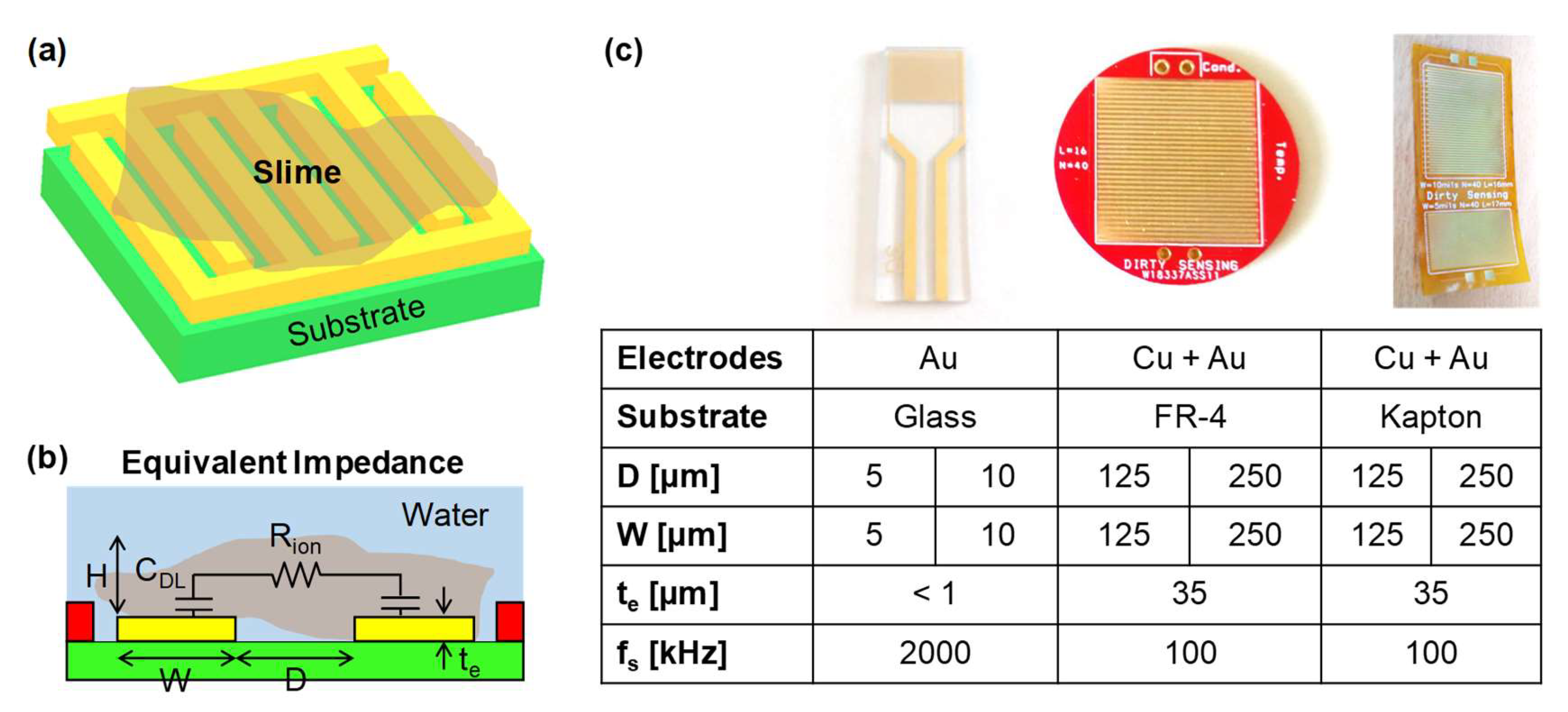
3.1. Slime Sensor
3.2. Other Chemo-Physical Sensors
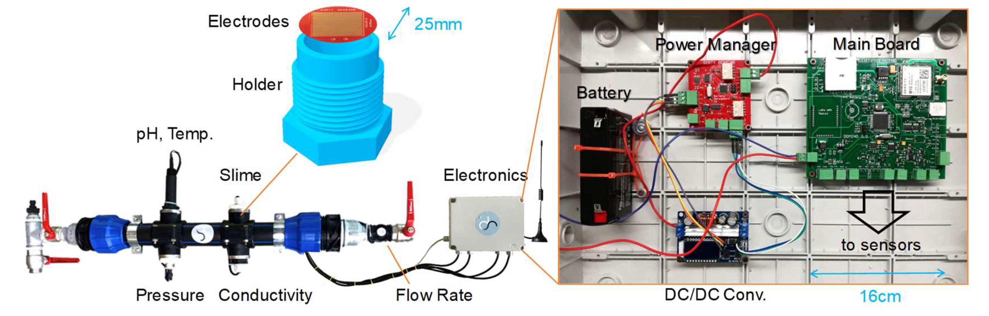
3.3. Complete Sensing Node
4. Electronics Design
5. Experimental Results and Discussion
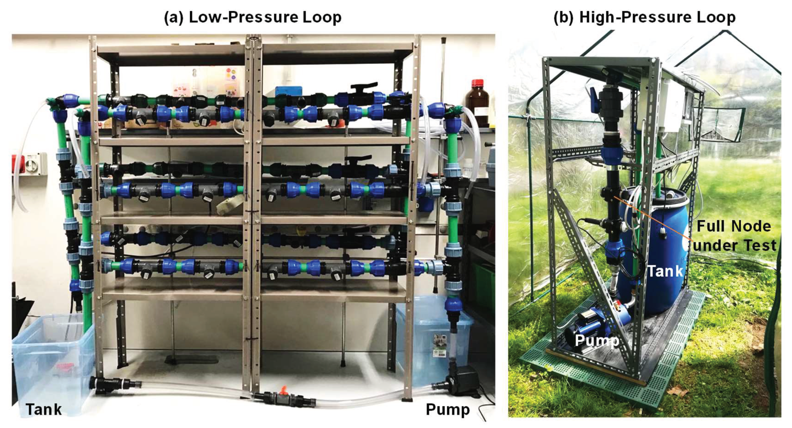
5.1. Laboratory Characterization of the Slime Monitor
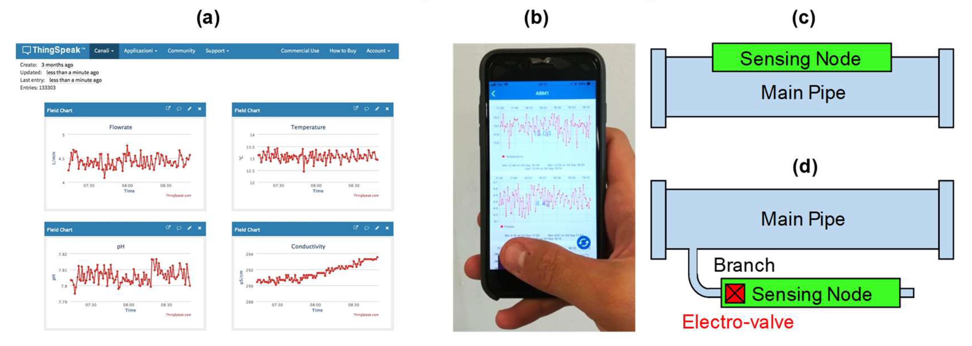
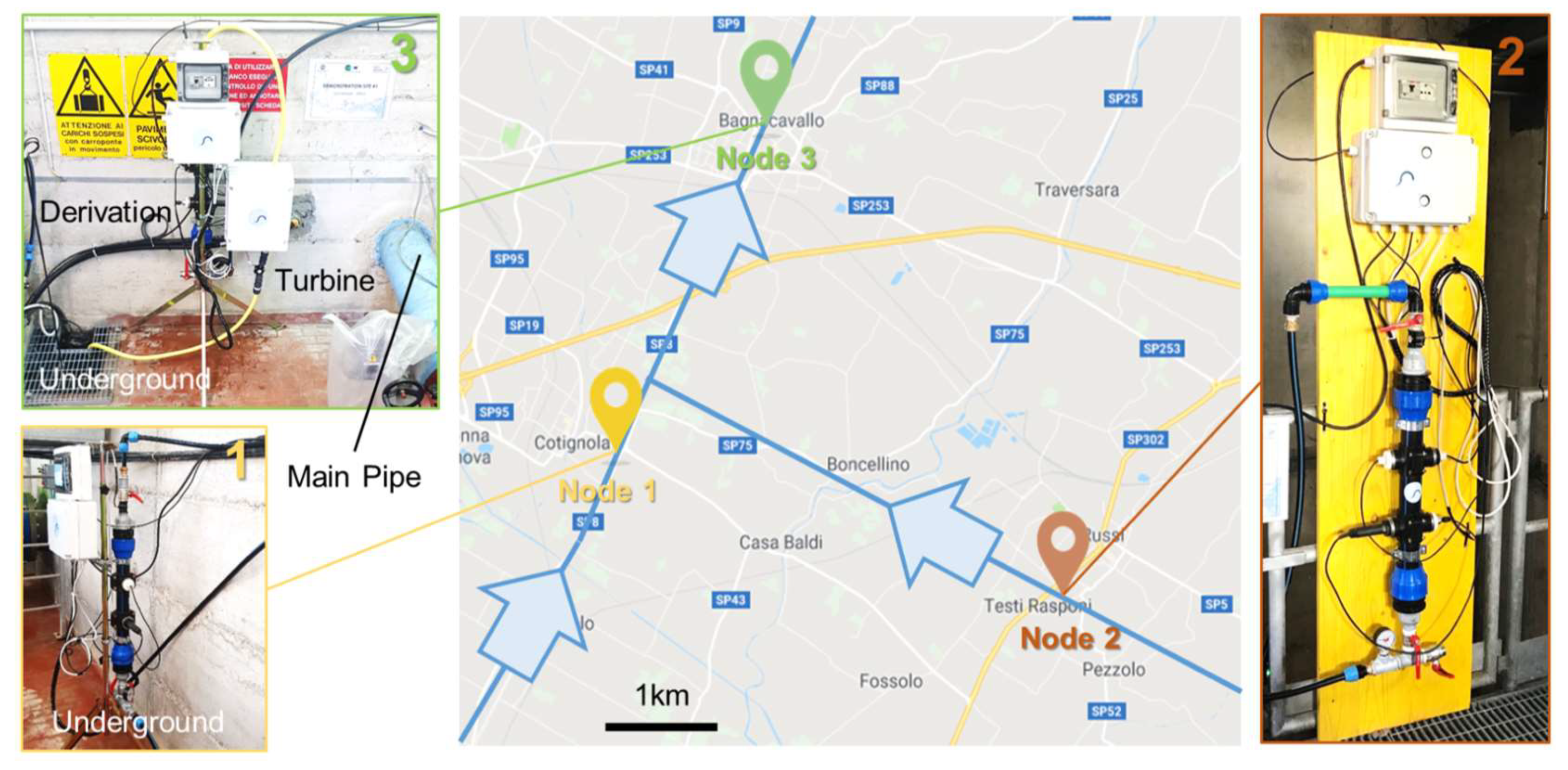
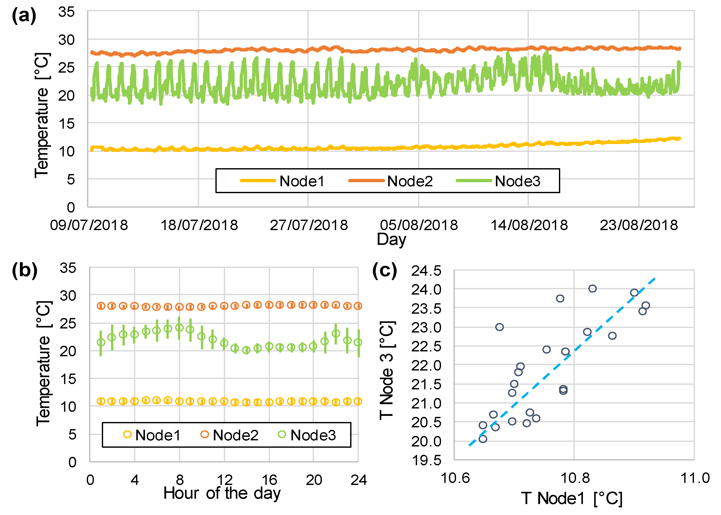
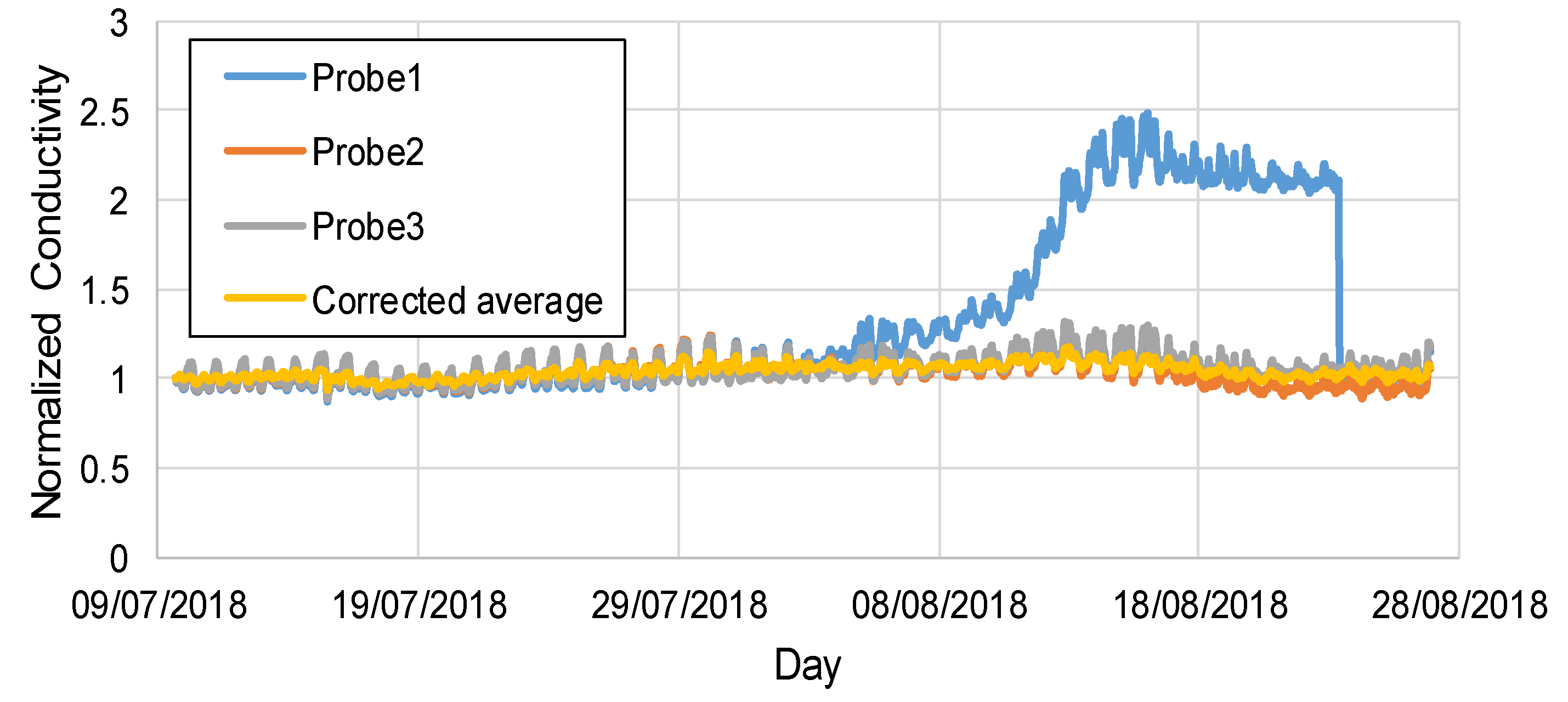
5.2. Field Validation of a Pilot Network
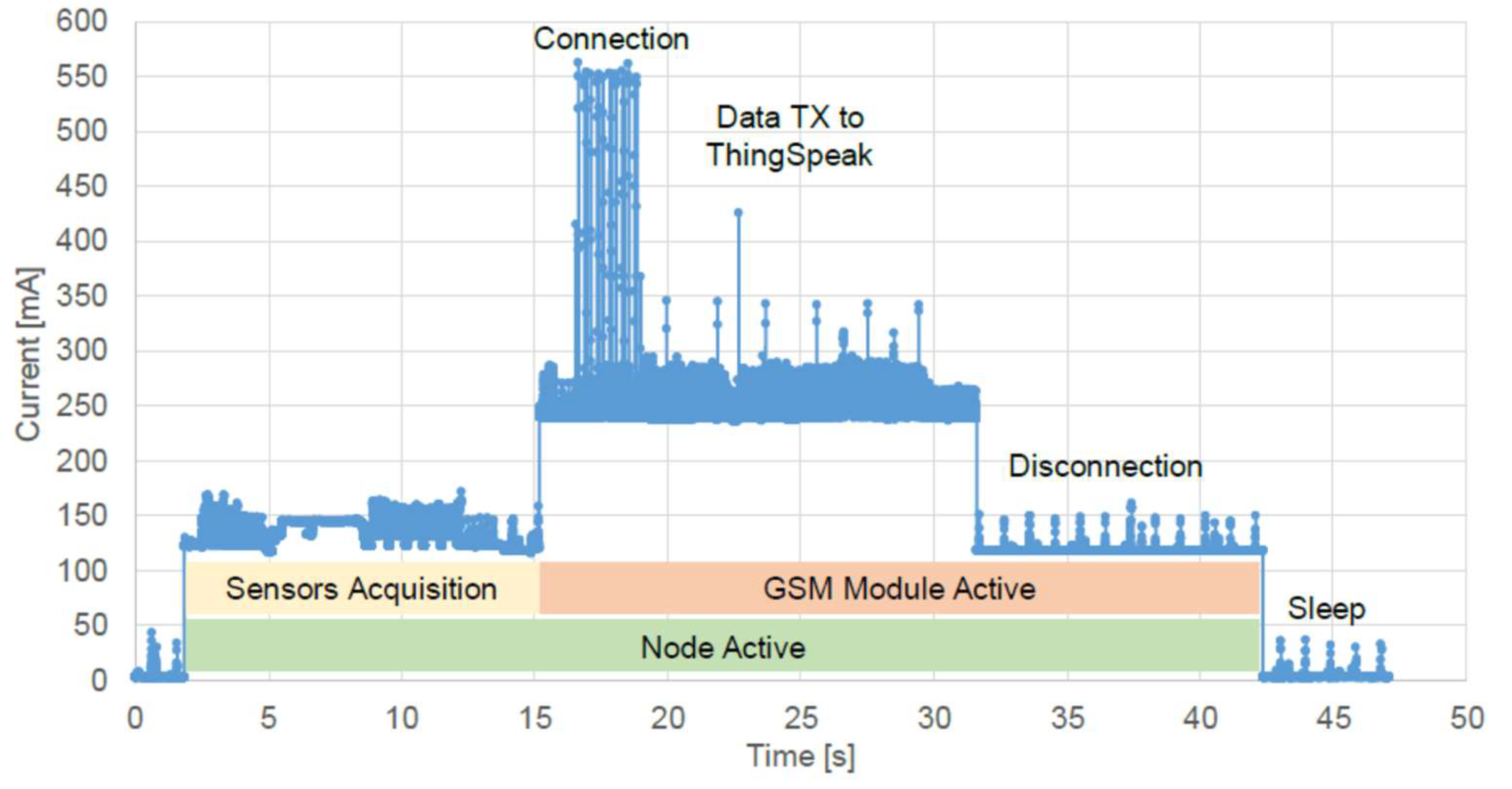
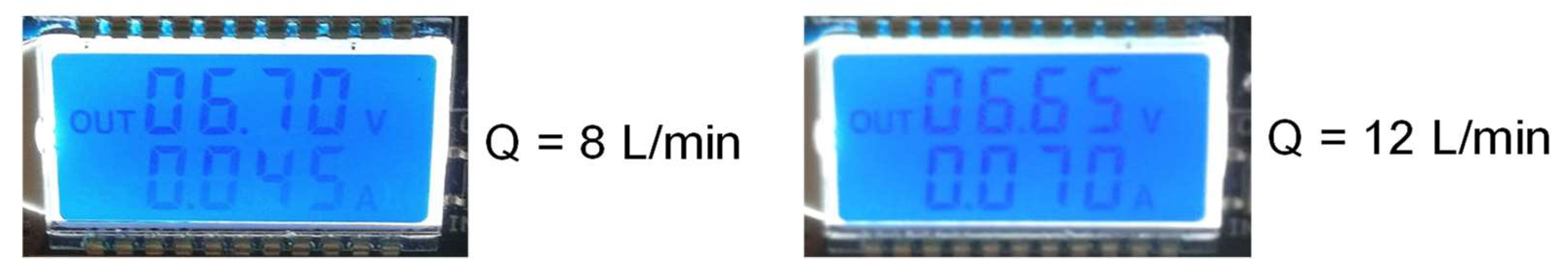
5.3. Energy Harvesting
6. Conclusions
Author Contributions
Funding
Acknowledgments
Conflicts of Interest
References
- Zulkifli, S.N.; Rahim, H.A.; Lau, W.-J. Detection of contaminants in water supply: A review on state-of-the-art monitoring technologies and their applications. Sens. Actuators B Chem. 2018, 255, 2657–2689. [Google Scholar] [CrossRef]
- Lambrou, T.P.; Anastasiou, C.C.; Panayiotou, C.G.; Polycarpou, M.M. A Low-Cost Sensor Network for Real-Time Monitoring and Contamination Detection in Drinking Water Distribution Systems. IEEE Sens. J. 2014, 14, 2765–2772. [Google Scholar] [CrossRef]
- Almazyad, A.; Seddiq, Y.; Alotaibi, A.; Al-Nasheri, A.; BenSaleh, M.; Obeid, A.; Qasim, S. A Proposed Scalable Design and Simulation of Wireless Sensor Network-Based Long-Distance Water Pipeline Leakage Monitoring System. Sensors 2014, 14, 3557–3577. [Google Scholar] [CrossRef] [PubMed] [Green Version]
- Xu, G.; Shen, W.; Wang, X. Applications of Wireless Sensor Networks in Marine Environment Monitoring: A Survey. Sensors 2014, 14, 16932–16954. [Google Scholar] [CrossRef] [PubMed] [Green Version]
- Albaladejo, C.; Soto, F.; Torres, R.; Sánchez, P.; López, J.A. A Low-Cost Sensor Buoy System for Monitoring Shallow Marine Environments. Sensors 2012, 12, 9613–9634. [Google Scholar] [CrossRef] [PubMed]
- Albaladejo, C.; Sánchez, P.; Iborra, A.; Soto, F.; López, J.A.; Torres, R. Wireless Sensor Networks for Oceanographic Monitoring: A Systematic Review. Sensors 2010, 10, 6948–6968. [Google Scholar] [CrossRef] [PubMed]
- Kotamäki, N.; Thessler, S.; Koskiaho, J.; Hannukkala, A.; Huitu, H.; Huttula, T.; Havento, J.; Järvenpää, M. Wireless in-situ Sensor Network for Agriculture and Water Monitoring on a River Basin Scale in Southern Finland: Evaluation from a Data User’s Perspective. Sensors 2009, 9, 2862–2883. [Google Scholar] [CrossRef]
- Kadir, E.A.; Siswanto, A.; Rosa, S.L.; Syukur, A.; Irie, H.; Othman, M. Smart Sensor Node of WSNs for River Water Pollution Monitoring System. In Proceedings of the 2019 International Conference on Advanced Communication Technologies and Networking (CommNet), Rabat, Morocco, 12–14 April 2019; IEEE: Rabat, Morocco, 2019; pp. 1–5. [Google Scholar]
- Postolache, O.A.; Girao, P.M.B.S.; Pereira, J.M.D.; Ramos, H.M.G. Self-Organizing Maps Application in a Remote Water Quality Monitoring System. IEEE Trans. Instrum. Meas. 2005, 54, 322–329. [Google Scholar] [CrossRef]
- Jiang, P.; Xia, H.; He, Z.; Wang, Z. Design of a Water Environment Monitoring System Based on Wireless Sensor Networks. Sensors 2009, 9, 6411–6434. [Google Scholar] [CrossRef] [Green Version]
- Tuna, G.; Arkoc, O.; Gulez, K. Continuous Monitoring of Water Quality Using Portable and Low-Cost Approaches. Int. J. Distrib. Sens. Netw. 2013, 9, 249598. [Google Scholar] [CrossRef]
- Dong, J.; Wang, G.; Yan, H.; Xu, J.; Zhang, X. A survey of smart water quality monitoring system. Environ. Sci. Pollut. Res. 2015, 22, 4893–4906. [Google Scholar] [CrossRef] [PubMed]
- Geetha, S.; Gouthami, S. Internet of things enabled real time water quality monitoring system. Smart Water 2016, 2, 1. [Google Scholar] [CrossRef]
- Japitana, M.V.; Palconit, E.V.; Demetillo, A.T.; Burce, M.E.C.; Taboada, E.B.; Abundo, M.L.S. Integrated Technologies for Low Cost Environmental Monitoring in the Water Bodies of the Philippines: A Review. Nat. Environ. Pollut. Technol. 2018, 17, 13. [Google Scholar]
- Metje, N.; Chapman, D.N.; Cheneler, D.; Ward, M.; Thomas, A.M. Smart Pipes—Instrumented Water Pipes, Can This Be Made a Reality? Sensors 2011, 11, 7455–7475. [Google Scholar] [CrossRef] [Green Version]
- Ali, H.; Choi, J. A Review of Underground Pipeline Leakage and Sinkhole Monitoring Methods Based on Wireless Sensor Networking. Sustainability 2019, 11, 4007. [Google Scholar] [CrossRef] [Green Version]
- Stoianov, I.; Nachman, L.; Madden, S.; Tokmouline, T. PIPENET: A Wireless Sensor Network for Pipeline Monitoring. In Proceedings of the 2007 6th International Symposium on Information Processing in Sensor Networks, Cambridge, MA, USA, 25–27 April 2007; IEEE: Cambridge, MA, USA, 2007; pp. 264–273. [Google Scholar]
- Prest, E.I.; Hammes, F.; van Loosdrecht, M.C.M.; Vrouwenvelder, J.S. Biological Stability of Drinking Water: Controlling Factors, Methods, and Challenges. Front. Microbiol. 2016, 7, 45. [Google Scholar] [CrossRef]
- Banna, M.H.; Imran, S.; Francisque, A.; Najjaran, H.; Sadiq, R.; Rodriguez, M.; Hoorfar, M. Online Drinking Water Quality Monitoring: Review on Available and Emerging Technologies. Crit. Rev. Environ. Sci. Technol. 2014, 44, 1370–1421. [Google Scholar] [CrossRef]
- Wingender, J.; Flemming, H.-C. Biofilms in drinking water and their role as reservoir for pathogens. Int. J. Hyg. Environ. Health 2011, 214, 417–423. [Google Scholar] [CrossRef]
- Richards, C.S.; Wang, F.; Becker, W.C.; Edwards, M.A. A 21st-Century Perspective on Calcium Carbonate Formation in Potable Water Systems. Environ. Eng. Sci. 2018, 35, 143–158. [Google Scholar] [CrossRef]
- Chung, W.S.; Yu, M.J.; Lee, H.D. Prediction of corrosion rates of water distribution pipelines according to aggressive corrosive water in Korea. Water Sci. Technol. 2004, 49, 19–26. [Google Scholar] [CrossRef]
- Delauney, L.; Compère, C.; Lehaitre, M. Biofouling protection for marine environmental sensors. Ocean Sci. 2010, 6, 503–511. [Google Scholar] [CrossRef] [Green Version]
- Aisopou, A.; Stoianov, I.; Graham, N.J.D. In-pipe water quality monitoring in water supply systems under steady and unsteady state flow conditions: A quantitative assessment. Water Res. 2012, 46, 235–246. [Google Scholar] [CrossRef] [PubMed]
- Kim, K.; Myung, H. Sensor Node for Remote Monitoring of Waterborne Disease-Causing Bacteria. Sensors 2015, 15, 10569–10579. [Google Scholar] [CrossRef] [PubMed] [Green Version]
- Available online: https://www.istat.it/it/files/2019/03/Testo-integrale_Report_Acqua_2019.pdf (accessed on 19 January 2020).
- Olatinwo, S.O.; Joubert, T.-H. Energy Efficient Solutions in Wireless Sensor Systems for Water Quality Monitoring: A Review. IEEE Sens. J. 2019, 19, 1596–1625. [Google Scholar] [CrossRef]
- Becker, P.; Folkmer, B.; Goepfert, R.; Hoffmann, D.; Willmann, A.; Manoli, Y. Energy Autonomous Wireless Water Meter with Integrated Turbine Driven Energy Harvester. J. Phys. Conf. Ser. 2013, 476, 012046. [Google Scholar] [CrossRef]
- Li, X.J.; Chong, P.H.J. Design and Implementation of a Self-Powered Smart Water Meter. Sensors 2019, 19, 4177. [Google Scholar] [CrossRef] [Green Version]
- Malavasi, S.; Rossi, M.M.A.; Ferrarese, G. GreenValve: Hydrodynamics and applications of the control valve for energy harvesting. Urban Water J. 2018, 15, 200–209. [Google Scholar] [CrossRef]
- Boccalero, G.; Boragno, C.; Caviglia, D.; Morasso, R. FLEHAP: A Wind Powered Supply for Autonomous Sensor Nodes. JSAN 2016, 5, 15. [Google Scholar] [CrossRef] [Green Version]
- Carminati, M.; Ferrari, G.; Sampietro, M. Emerging miniaturized technologies for airborne particulate matter pervasive monitoring. Measurement 2017, 101, 250–256. [Google Scholar] [CrossRef]
- Montagnani, G.L.; Carminati, M.; Lavelli, E.; Morandi, G.; Rizzacasa, P.; Fiorini, C. SiPM-Based Scrap Metal Radioactivity Detector Embeddable in Lifting Electromagnets. In Proceedings of the 2018 IEEE Nuclear Science Symposium and Medical Imaging Conference Proceedings (NSS/MIC), Sydney, Australia, 10–17 November 2018; IEEE: Sydney, Australia, 2018; pp. 1–3. [Google Scholar]
- Keller, O.; Benoit, M.; Müller, A.; Schmeling, S. Smartphone and Tablet-Based Sensing of Environmental Radioactivity: Mobile Low-Cost Measurements for Monitoring, Citizen Science, and Educational Purposes. Sensors 2019, 19, 4264. [Google Scholar] [CrossRef] [Green Version]
- Colli, M.; Stagnaro, M.; Caridi, A.; Lanza, L.G.; Randazzo, A.; Pastorino, M.; Caviglia, D.D.; Delucchi, A. A Field Assessment of a Rain Estimation System Based on Satellite-to-Earth Microwave Links. IEEE Trans. Geosci. Remote Sens. 2019, 57, 2864–2875. [Google Scholar] [CrossRef]
- Carminati, M.; Ferrari, G.; Vahey, M.D.; Voldman, J.; Sampietro, M. Miniaturized Impedance Flow Cytometer: Design Rules and Integrated Readout. IEEE Trans. Biomed. Circuits Syst. 2017, 11, 1438–1449. [Google Scholar] [CrossRef] [PubMed]
- Igreja, R.; Dias, C.J. Analytical evaluation of the interdigital electrodes capacitance for a multi-layered structure. Sens. Actuators A Phys. 2004, 112, 291–301. [Google Scholar] [CrossRef]
- Mezzera, L.; Carminati, M.; Di Mauro, M.; Turolla, A.; Tizzoni, M.; Antonelli, M. A 7-Parameter Platform for Smart and Wireless Networks Monitoring On-Line Water Quality. In Proceedings of the 2018 25th IEEE International Conference on Electronics, Circuits and Systems (ICECS), Bordeaux, France, 9–12 December 2018; IEEE: Bordeaux, France, 2018; pp. 709–712. [Google Scholar]
- Vergani, M.; Carminati, M.; Ferrari, G.; Landini, E.; Caviglia, C.; Heiskanen, A.; Comminges, C.; Zor, K.; Sabourin, D.; Dufva, M.; et al. Multichannel Bipotentiostat Integrated With a Microfluidic Platform for Electrochemical Real-Time Monitoring of Cell Cultures. IEEE Trans. Biomed. Circuits Syst. 2012, 6, 498–507. [Google Scholar] [CrossRef] [Green Version]
- Turolla, A.; Di Mauro, M.; Mezzera, L.; Antonelli, M.; Carminati, M. Development of a Miniaturized and Selective Impedance Sensor for Real-Time Slime Monitoring in Pipes and Tanks. Sens. Actuators B Chem. 2019, 281, 288–295. [Google Scholar] [CrossRef]
- Carminati, M.; Mezzera, L.; Turolla, A.; Pani, G.; Tizzoni, M.; Di Mauro, M.; Antonelli, M. Flexible Impedance Sensor for In-Line Monitoring of Water and Beverages. In Proceedings of the 2019 IEEE International Symposium on Circuits and Systems (ISCAS), Sapporo, Japan, 26–29 May 2019; IEEE: Sapporo, Japan, 2019; pp. 1–4. [Google Scholar]
- Carminati, M.; Luzzatto-Fegiz, P. Conduino: Affordable and high-resolution multichannel water conductivity sensor using micro USB connectors. Sens. Actuators B Chem. 2017, 251, 1034–1041. [Google Scholar] [CrossRef]
- Carminati, M.; Ferrari, G.; Grassetti, R.; Sampietro, M. Real-Time Data Fusion and MEMS Sensors Fault Detection in an Aircraft Emergency Attitude Unit Based on Kalman Filtering. IEEE Sens. J. 2012, 12, 2984–2992. [Google Scholar] [CrossRef] [Green Version]
- Carminati, M.; Mezzera, L.; Ferrari, G.; Sampietro, M.; Turolla, A.; Di Mauro, M.; Antonelli, M. A Smart Sensing Node for Pervasive Water Quality Monitoring with Anti-Fouling Self-Diagnostics. In Proceedings of the 2018 IEEE International Symposium on Circuits and Systems (ISCAS), Florence, Italy, 27–30 May 2018; IEEE: Florence, Italy, 2018; pp. 1–5. [Google Scholar]


© 2020 by the authors. Licensee MDPI, Basel, Switzerland. This article is an open access article distributed under the terms and conditions of the Creative Commons Attribution (CC BY) license (http://creativecommons.org/licenses/by/4.0/).
Share and Cite
Carminati, M.; Turolla, A.; Mezzera, L.; Di Mauro, M.; Tizzoni, M.; Pani, G.; Zanetto, F.; Foschi, J.; Antonelli, M. A Self-Powered Wireless Water Quality Sensing Network Enabling Smart Monitoring of Biological and Chemical Stability in Supply Systems. Sensors 2020, 20, 1125. https://0-doi-org.brum.beds.ac.uk/10.3390/s20041125
Carminati M, Turolla A, Mezzera L, Di Mauro M, Tizzoni M, Pani G, Zanetto F, Foschi J, Antonelli M. A Self-Powered Wireless Water Quality Sensing Network Enabling Smart Monitoring of Biological and Chemical Stability in Supply Systems. Sensors. 2020; 20(4):1125. https://0-doi-org.brum.beds.ac.uk/10.3390/s20041125
Chicago/Turabian StyleCarminati, Marco, Andrea Turolla, Lorenzo Mezzera, Michele Di Mauro, Marco Tizzoni, Gaia Pani, Francesco Zanetto, Jacopo Foschi, and Manuela Antonelli. 2020. "A Self-Powered Wireless Water Quality Sensing Network Enabling Smart Monitoring of Biological and Chemical Stability in Supply Systems" Sensors 20, no. 4: 1125. https://0-doi-org.brum.beds.ac.uk/10.3390/s20041125