A Bluetooth-Low-Energy-Based Detection and Warning System for Vulnerable Road Users in the Blind Spot of Vehicles


Abstract
:1. Introduction and Related Work
2. Design
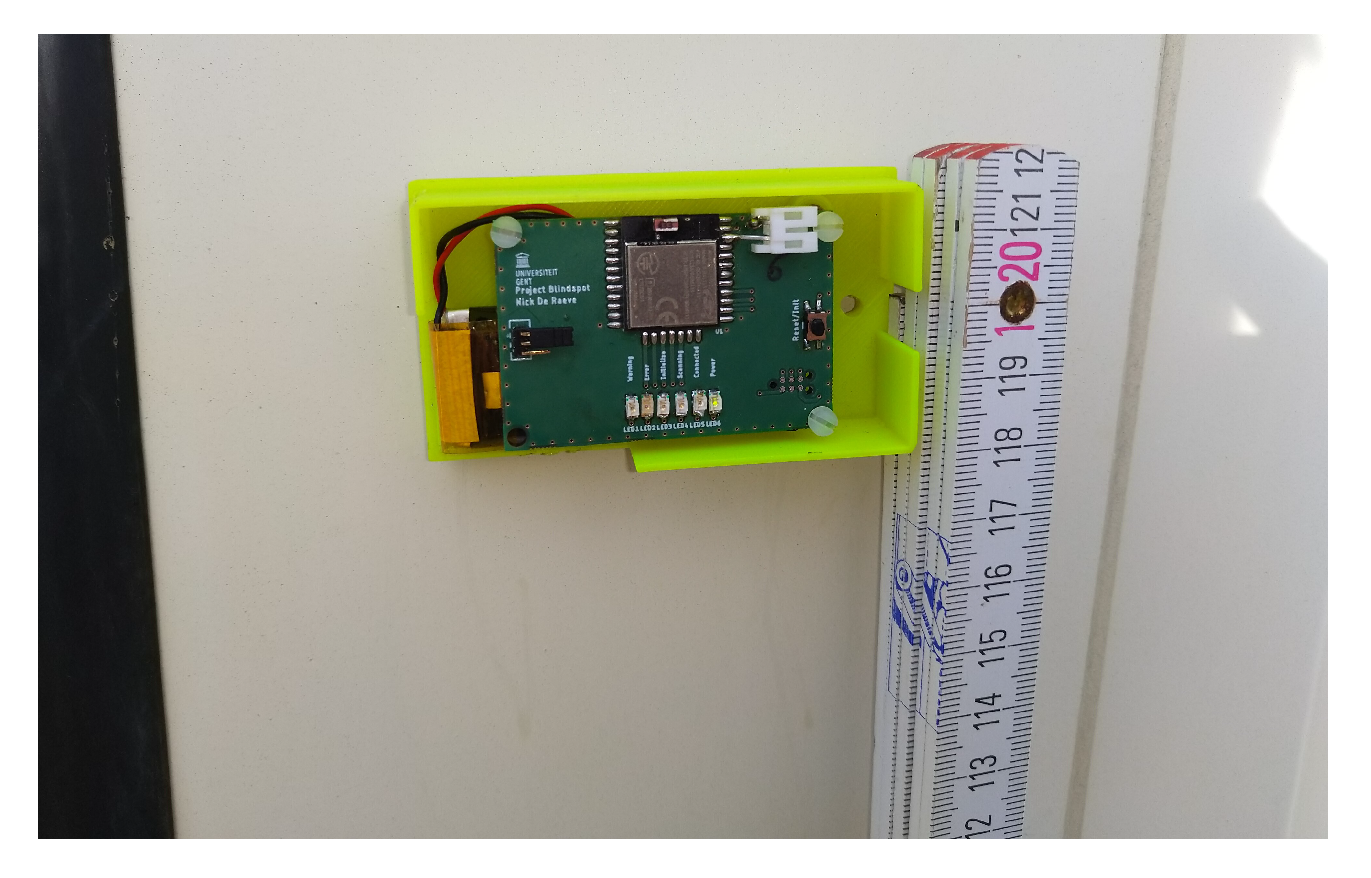
2.1. Hardware Implementation
2.2. Software
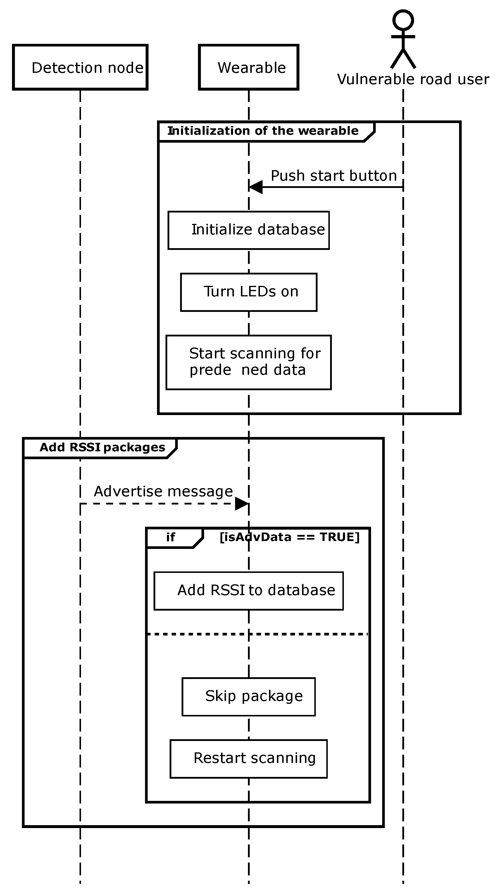
2.2.1. Wearable
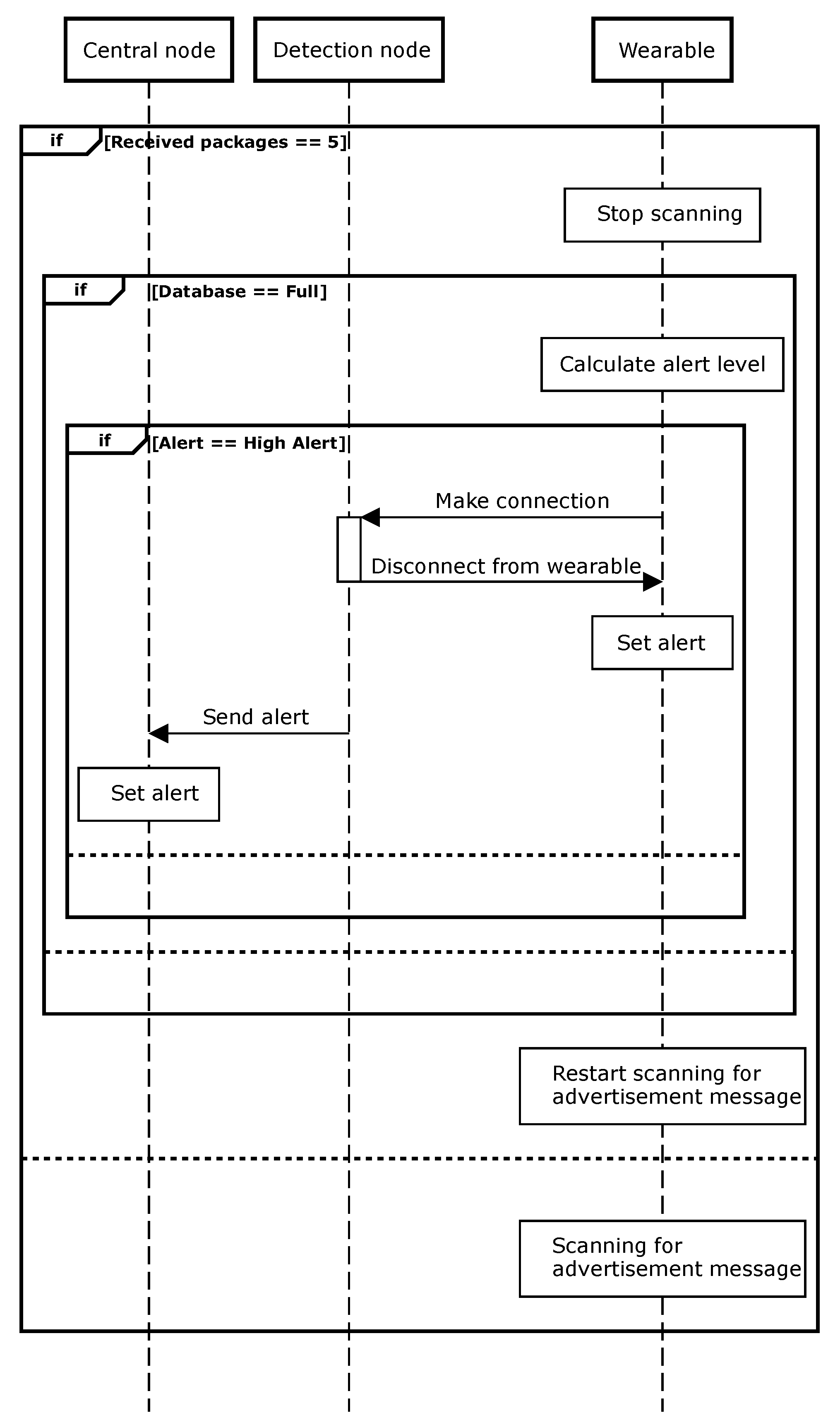
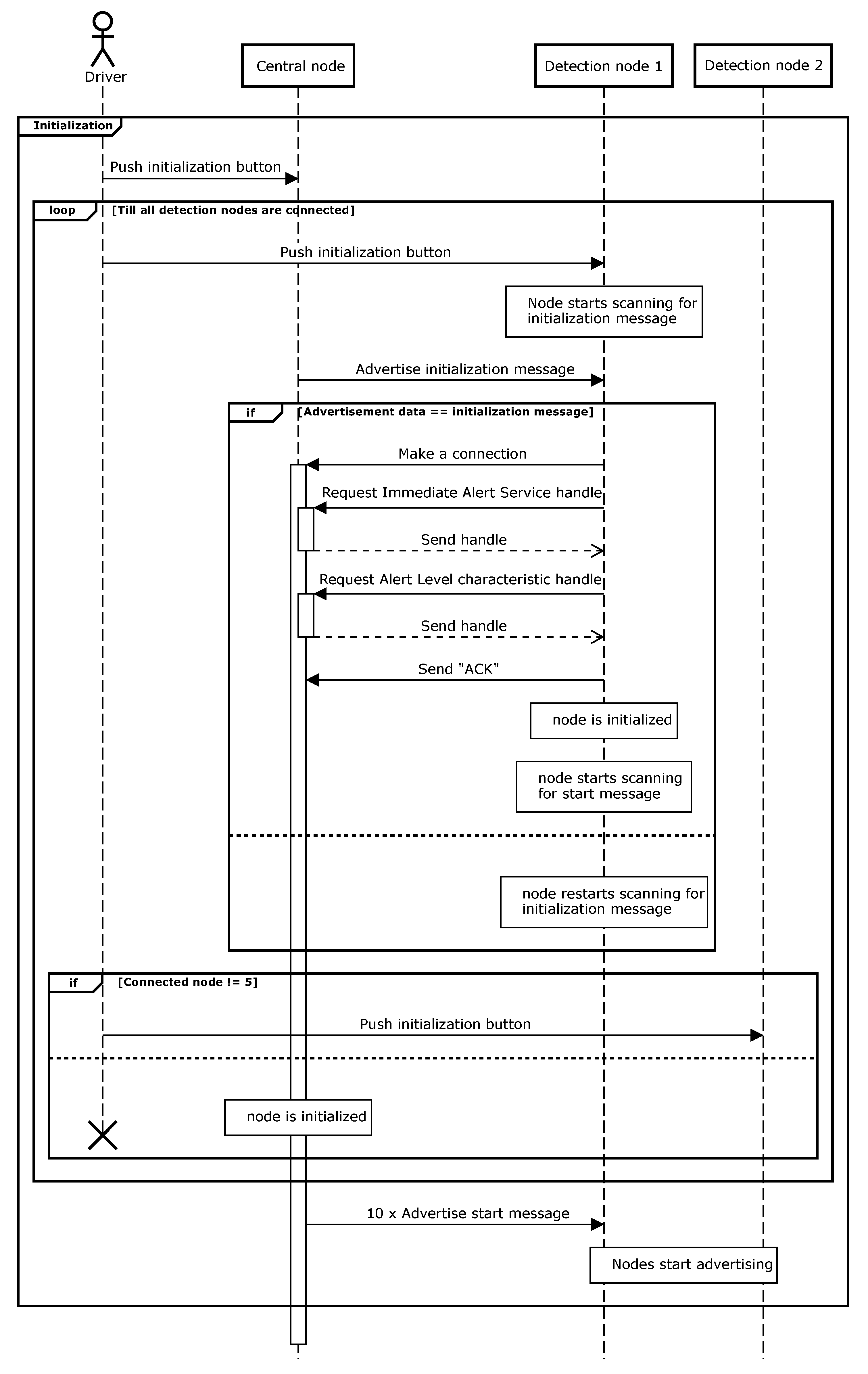
2.2.2. Detection and Central Node
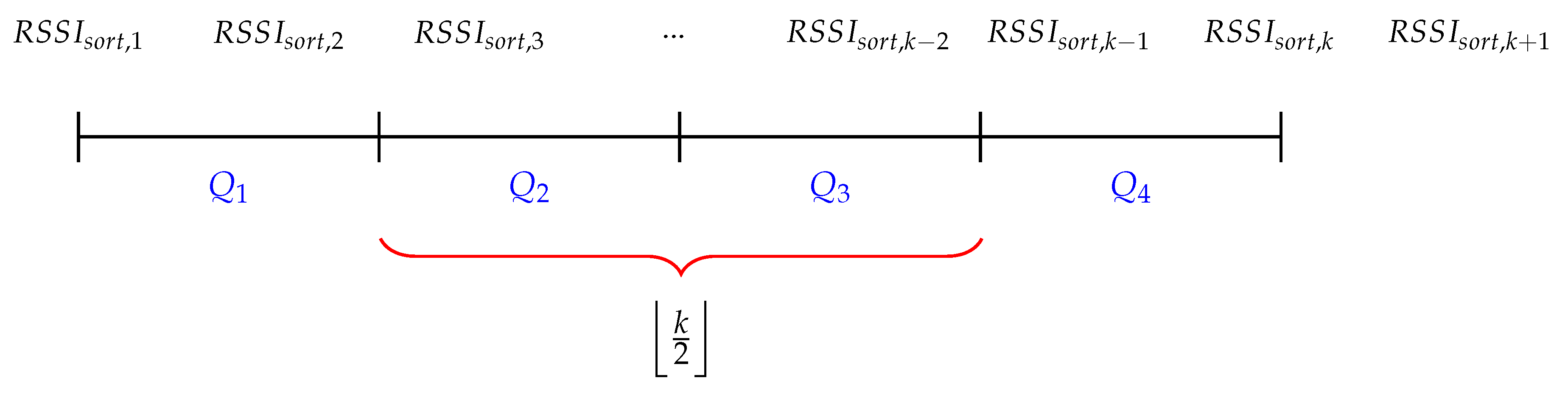
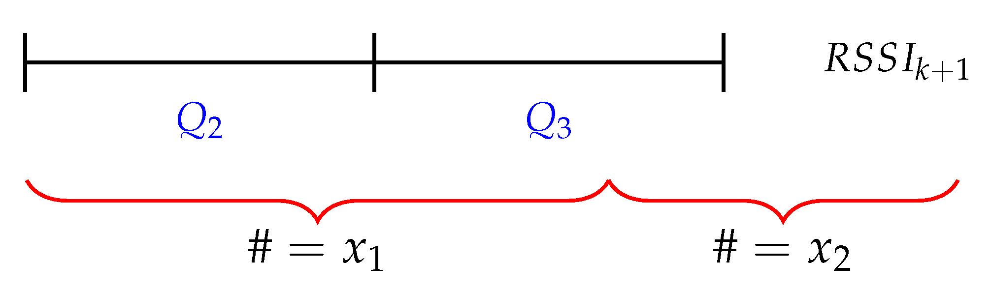
2.3. Filtering
3. Measurements
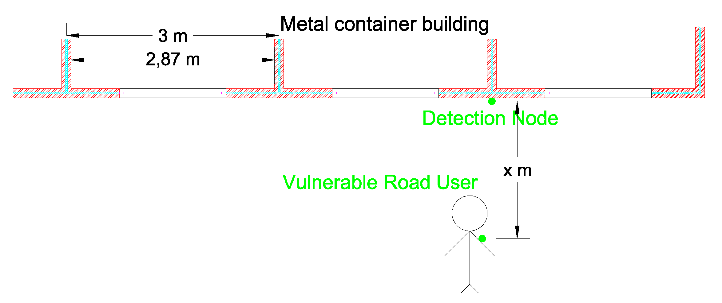
3.1. Measurement Setup
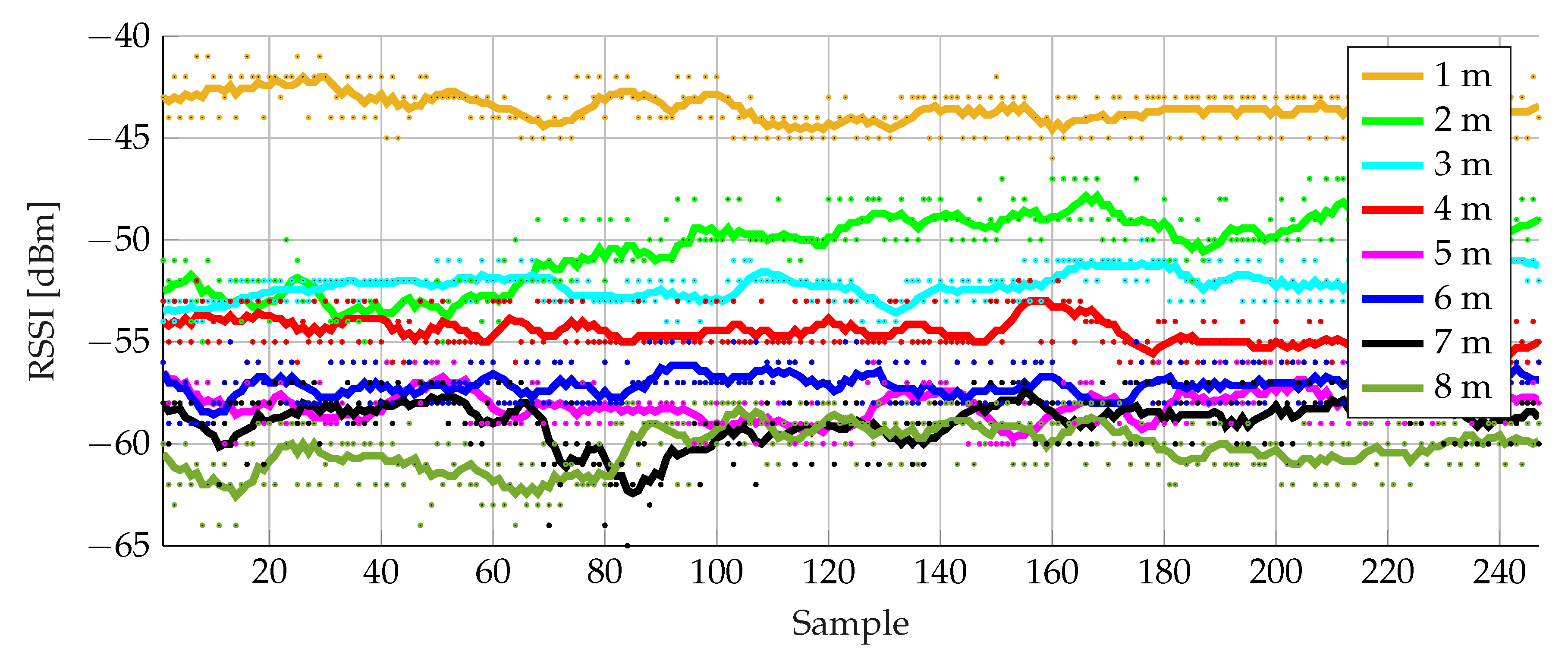
3.1.1. Static RSSI Measurement
3.1.2. Dynamic RSSI Measurement
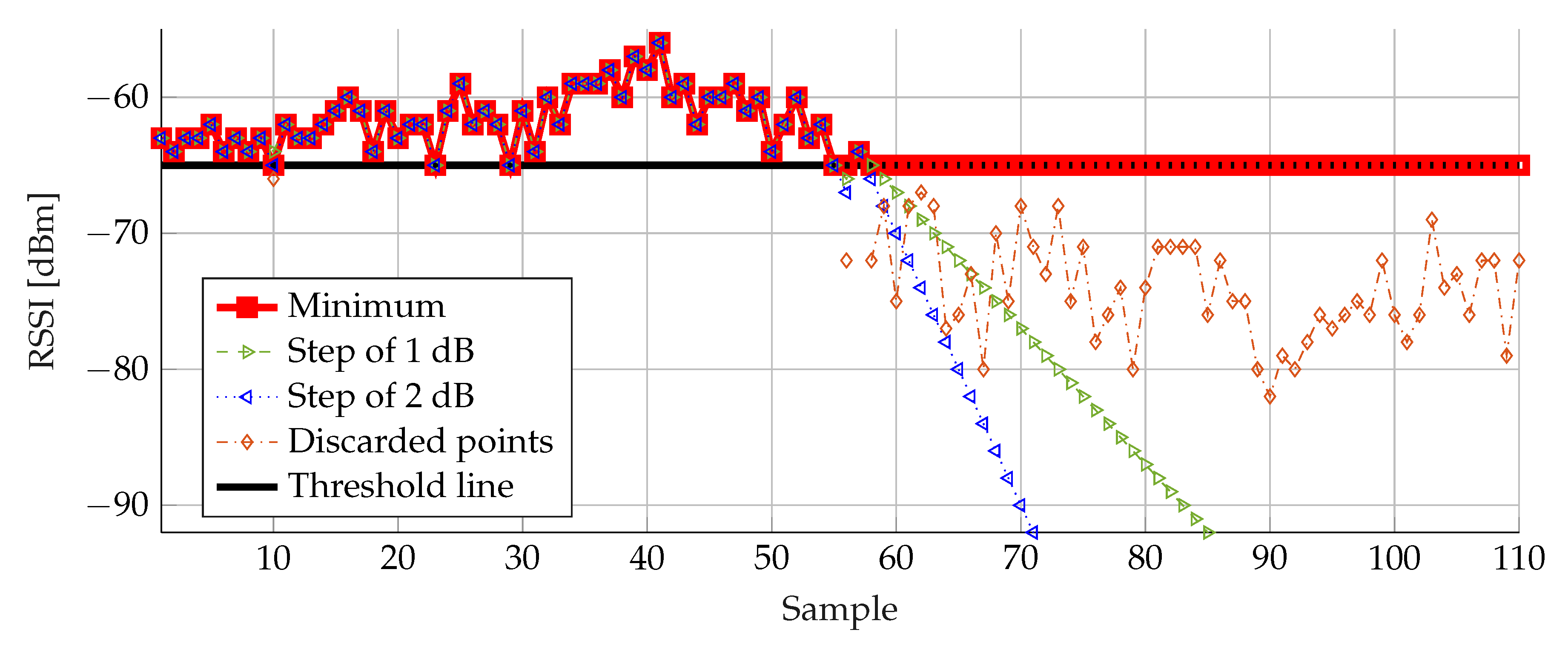
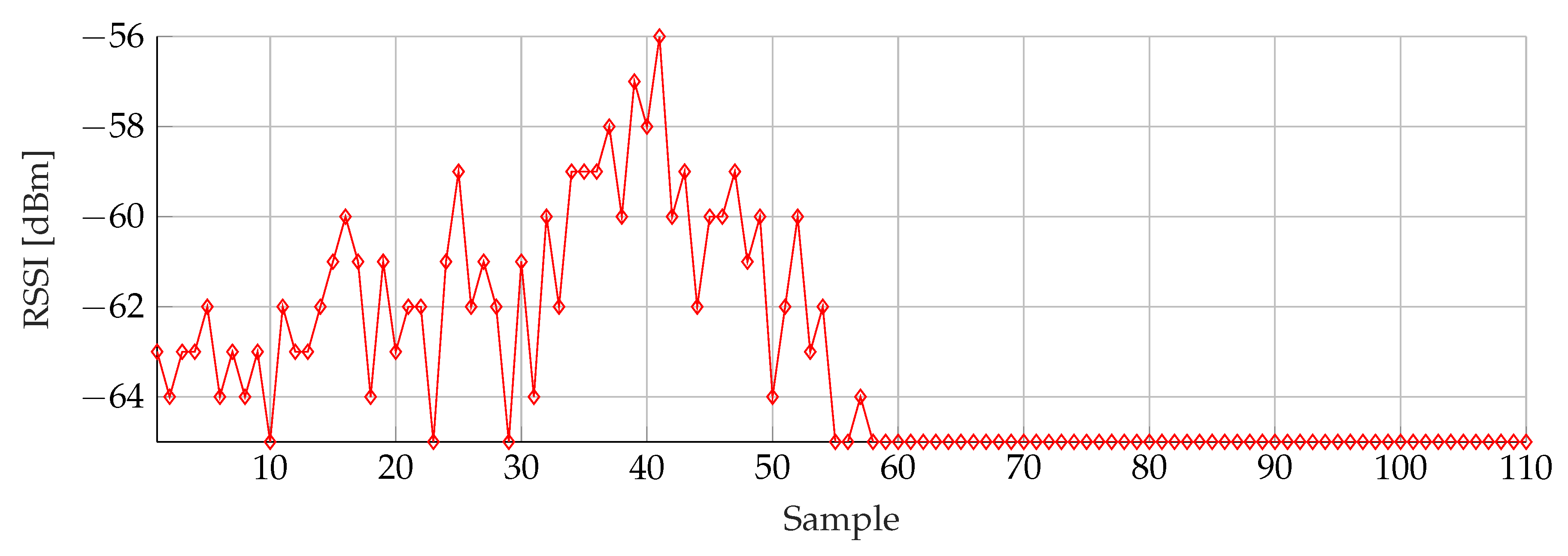
3.2. Threshold Filtering
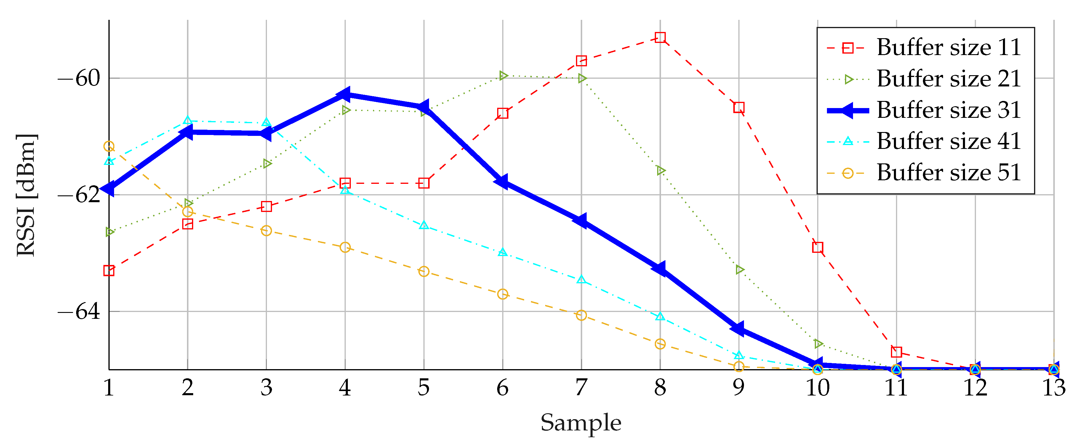
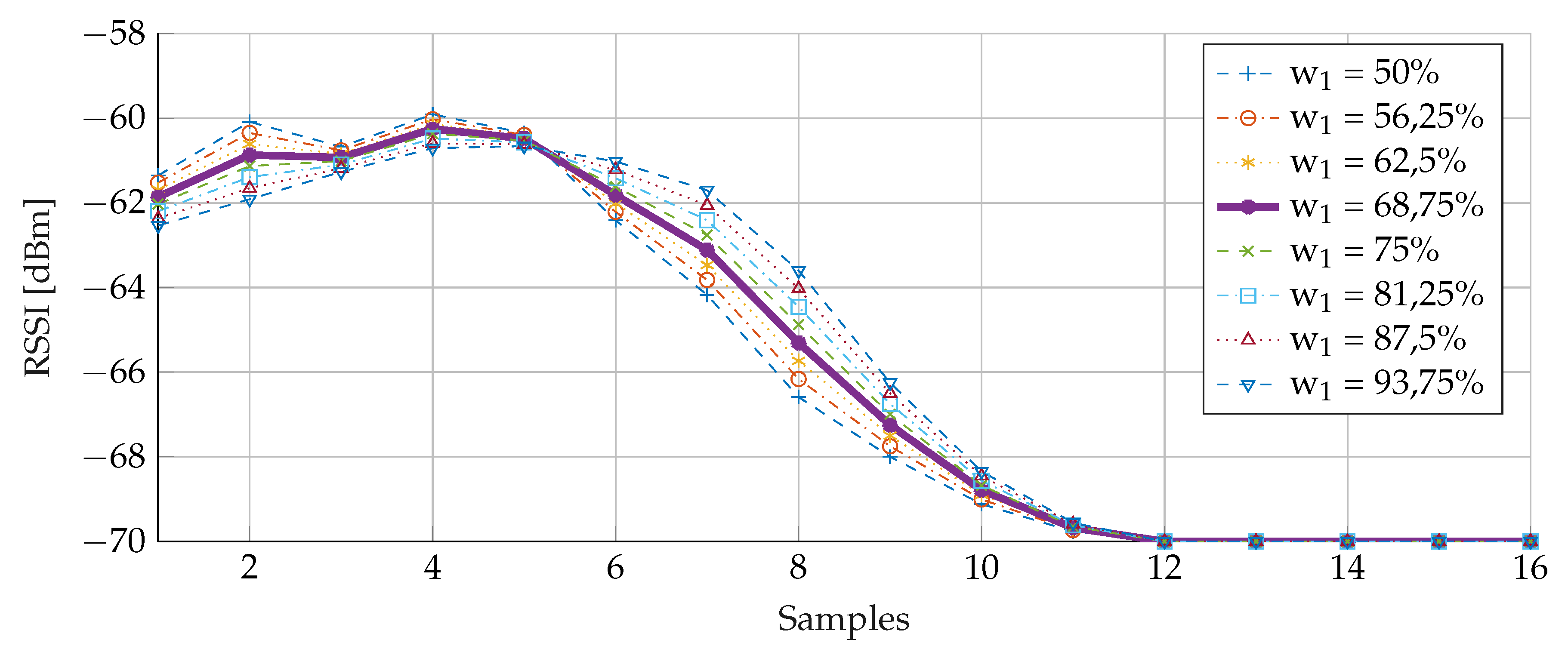
3.3. Weighted Average Filter with Sliding Window
3.4. Optimized Algorithm
4. Real-Life Measurements
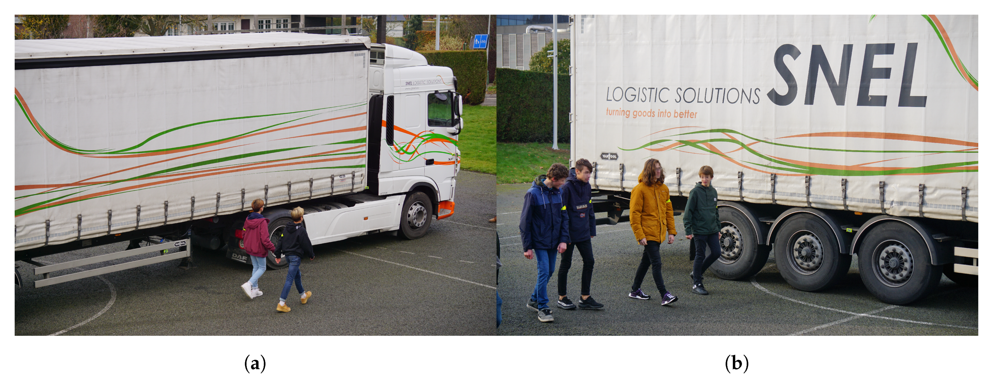
4.1. General Test
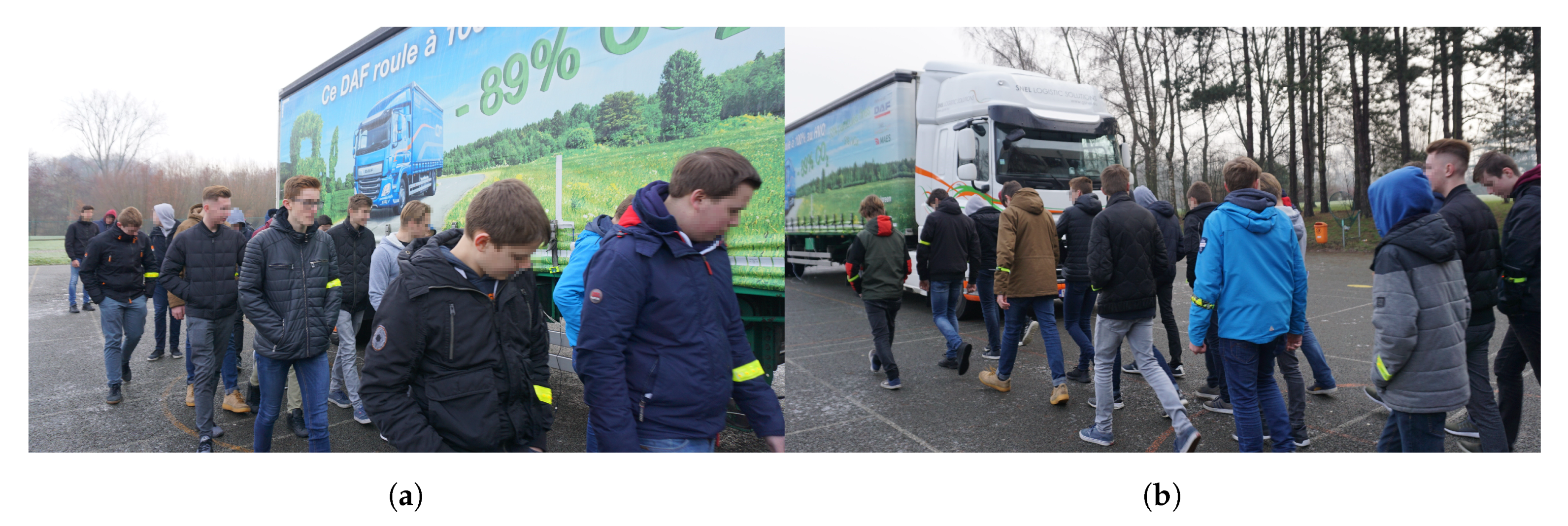
4.2. Large Group of People
4.3. Verification Measurement
5. Conclusions
Author Contributions
Funding
Acknowledgments
Conflicts of Interest
Abbreviations
| BLE | Bluetooth Low Energy |
| LED | Light Emitting Diode |
| LoS | Line-of-Sight |
| PCB | Printed Circuit Board |
| RSSI | Received Signal Strength Indicator |
| SWD | Serial Wire Debug |
References
- Veiligverkeer.be. Cijfers en Ongevallen Dode Hoek. Available online: https://www.veiligverkeer.be/inhoud/cijfers-en-ongevallen-dode-hoek/ (accessed on 7 May 2020).
- Chang, S.; Tsai, C.; Guo, J. A blind spot detection warning system based on Gabor filtering and optical flow for E-mirror applications. In Proceedings of the 2018 IEEE International Symposium on Circuits and Systems (ISCAS), Florence, Italy, 27–30 May 2018; pp. 1–5. [Google Scholar]
- Baek, J.W.; Lee, E.; Park, M.; Seo, D. Mono-camera based side vehicle detection for blind spot detection systems. In Proceedings of the 2015 Seventh International Conference on Ubiquitous and Future Networks, Sapporo, Japan, 7–10 July 2015; pp. 147–149. [Google Scholar] [CrossRef]
- Baek, S.; Kim, H.; Boo, K. Robust vehicle detection and tracking method for blind spot detection system by using vision sensors. In Proceedings of the 2014 Second World Conference on Complex Systems (WCCS), Agadir, Morocco, 10–12 November 2014; pp. 729–735. [Google Scholar] [CrossRef]
- Chen, Y.; Wu, B.; Huang, H.; Fan, C. A real-time vision system for nighttime vehicle detection and traffic surveillance. IEEE Trans. Ind. Electron. 2011, 58, 2030–2044. [Google Scholar] [CrossRef]
- Chen, C.T.; Chen, Y.S. Real-time approaching vehicle detection in blind spot area. In Proceedings of the 2009 12th International IEEE Conference on Intelligent Transportation Systems, St. Louis, MO, USA, 4–7 October 2009; pp. 1–6. [Google Scholar] [CrossRef]
- Liu, G.; Wang, L.; Zou, S. A radar-based blind spot detection and warning system for driver assistance. In Proceedings of the 2017 IEEE Second Advanced Information Technology, Electronic and Automation Control Conference (IAEAC), Chongqing, China, 25–26 March 2017; pp. 2204–2208. [Google Scholar] [CrossRef]
- VIAS. Ongevallen Met Vrachtwagens—Fase 1. Available online: https://www.vias.be/publications/Ongevallen%20met%20vrachtwagens%20%E2%80%93%20Fase%201/Ongevallen_met_vrachtwagens_%E2%80%93_Fase_1.pdf (accessed on 7 May 2020).
- VIAS. In-Depth Investigation of Crashes Involving Heavy Goods Vehicles. Available online: https://www.vias.be/publications/Ongevallen%20met%20vrachtwagens%20%E2%80%93%20Fase%202/Accidents_involving_trucks_%E2%80%93_Phase_2.pdf (accessed on 7 May 2020).
- Bulić, P.; Kojek, G.; Biasizzo, A. Data Transmission Efficiency in Bluetooth Low Energy Versions. Sensors 2019, 19, 3746. [Google Scholar] [CrossRef] [PubMed] [Green Version]
- Silicon Laboratories. BGM111 Blue Gecko Bluetooth Module Data Sheet. Available online: https://www.silabs.com/documents/public/data-sheets/BGM111_datasheet.pdf (accessed on 7 May 2020).
- Bluetooth Special Interest Group. Specification of the Bluetooth System, Covered Core Package Version 4.2. Available online: https://www.bluetooth.com/specifications/archived-specifications/ (accessed on 7 May 2020).
- ARM. Available online: https://www.arm.com/products/silicon-ip-cpu (accessed on 7 May 2020).
- TAG Connect. Available online: http://www.tag-connect.com/ (accessed on 7 May 2020).
- Silicon Laboratories. Programming Internal Flash Over the Serial Wire Debug Interface. Available online: https://www.silabs.com/documents/public/application-notes/an0062.pdf (accessed on 7 May 2020).
- J & A. Lithium-ion Polymer Battery, Specification Model: JA-803450P. Available online: https://www.olimex.com/Products/Power/BATTERY-LIPO1400mAh/resources/JA803450-Spec-Data-Sheet–J-A.pdf (accessed on 7 May 2020).
- Silicon Laboratories. Available online: https://www.silabs.com/products/development-tools/wireless/bluetooth/bluegecko-bluetooth-low-energy-module-wireless-starter-kit (accessed on 7 May 2020).
- Murata. Buzzer murata PKLCS1212E4001-R1. Available online: https://www.murata.com/en-eu/api/pdfdownloadapi?cate=cgsubSounders&partno=PKLCS1212E4001-R1 (accessed on 7 May 2020).
- Nikodem, M.; Bawiec, M. Experimental Evaluation of Advertisement-Based Bluetooth Low Energy Communication. Sensors 2019, 20, 107. [Google Scholar] [CrossRef] [PubMed] [Green Version]
- Li, G.; Geng, E.; Ye, Z.; Xu, Y.; Lin, J.; Pang, Y. Indoor Positioning Algorithm Based on the Improved RSSI Distance Model. Sensors 2018, 18, 2820. [Google Scholar] [CrossRef] [PubMed] [Green Version]
- Cannizzaro, D.; Zari, M.; Pagliari, D.J.; Patti, E.; Macii, E.; Poncino, M.; Acquaviva, A. A Comparison Analysis of BLE-based Algorithms for Localization in Industrial Environments. Electronics 2019, 9, 44. [Google Scholar] [CrossRef] [Green Version]
- Onofre, S.; Silvestre, P.M.; Pimentão, J.P.; Sousa, P. Surpassing Bluetooth Low Energy limitations on distance determination. In Proceedings of the 2016 IEEE International Power Electronics and Motion Control Conference (PEMC), Varna, Bulgaria, 25–28 September 2016; pp. 843–847. [Google Scholar] [CrossRef]


© 2020 by the authors. Licensee MDPI, Basel, Switzerland. This article is an open access article distributed under the terms and conditions of the Creative Commons Attribution (CC BY) license (http://creativecommons.org/licenses/by/4.0/).
Share and Cite
De Raeve, N.; de Schepper, M.; Verhaevert, J.; Van Torre, P.; Rogier, H. A Bluetooth-Low-Energy-Based Detection and Warning System for Vulnerable Road Users in the Blind Spot of Vehicles. Sensors 2020, 20, 2727. https://0-doi-org.brum.beds.ac.uk/10.3390/s20092727
De Raeve N, de Schepper M, Verhaevert J, Van Torre P, Rogier H. A Bluetooth-Low-Energy-Based Detection and Warning System for Vulnerable Road Users in the Blind Spot of Vehicles. Sensors. 2020; 20(9):2727. https://0-doi-org.brum.beds.ac.uk/10.3390/s20092727
Chicago/Turabian StyleDe Raeve, Nick, Matthias de Schepper, Jo Verhaevert, Patrick Van Torre, and Hendrik Rogier. 2020. "A Bluetooth-Low-Energy-Based Detection and Warning System for Vulnerable Road Users in the Blind Spot of Vehicles" Sensors 20, no. 9: 2727. https://0-doi-org.brum.beds.ac.uk/10.3390/s20092727