
Detecting Phase-Synchrony Connectivity Anomalies in EEG Signals. Application to Dyslexia Diagnosis

 , , ,
, , ,
Abstract
:1. Introduction
- Methods that characterize the statistical relationships between electrodes but in the same frequency band. In this way, Spectral Coherence (SC) provides a way to measure the synchronization between channels, which may indicate a connection from the functional point of view between the neuron clusters in the two areas involved [33]. Other connectivity measures can be computed from the phase angle differences between channels over time [21].
- Methods that characterize the statistical relationships between the activity in two channels at different frequency bands. The measure provided by these methods is commonly referred as Cross Frequency Coupling (CFC). Phase-Amplitude Coupling (PAC) is a representative and practical example for computing the CFC which has neural and physical implications [34].
- We use low level auditory stimuli to study the brain processes involved in language processing, instead of previous works that use only speech-based stimuli [22].
- Connectivity between brain areas is searched by means of phase synchronization between EEG channels, which is computed using the Circular Correlation.
- An anomaly detection approach has been implemented using a method that combines unsupervised learning by vector quantization and a Bayesian classifier. The proposed method allows working with not very large databases, overcomes the imbalance problem and reduces the overfitting.
2. Materials and Methods
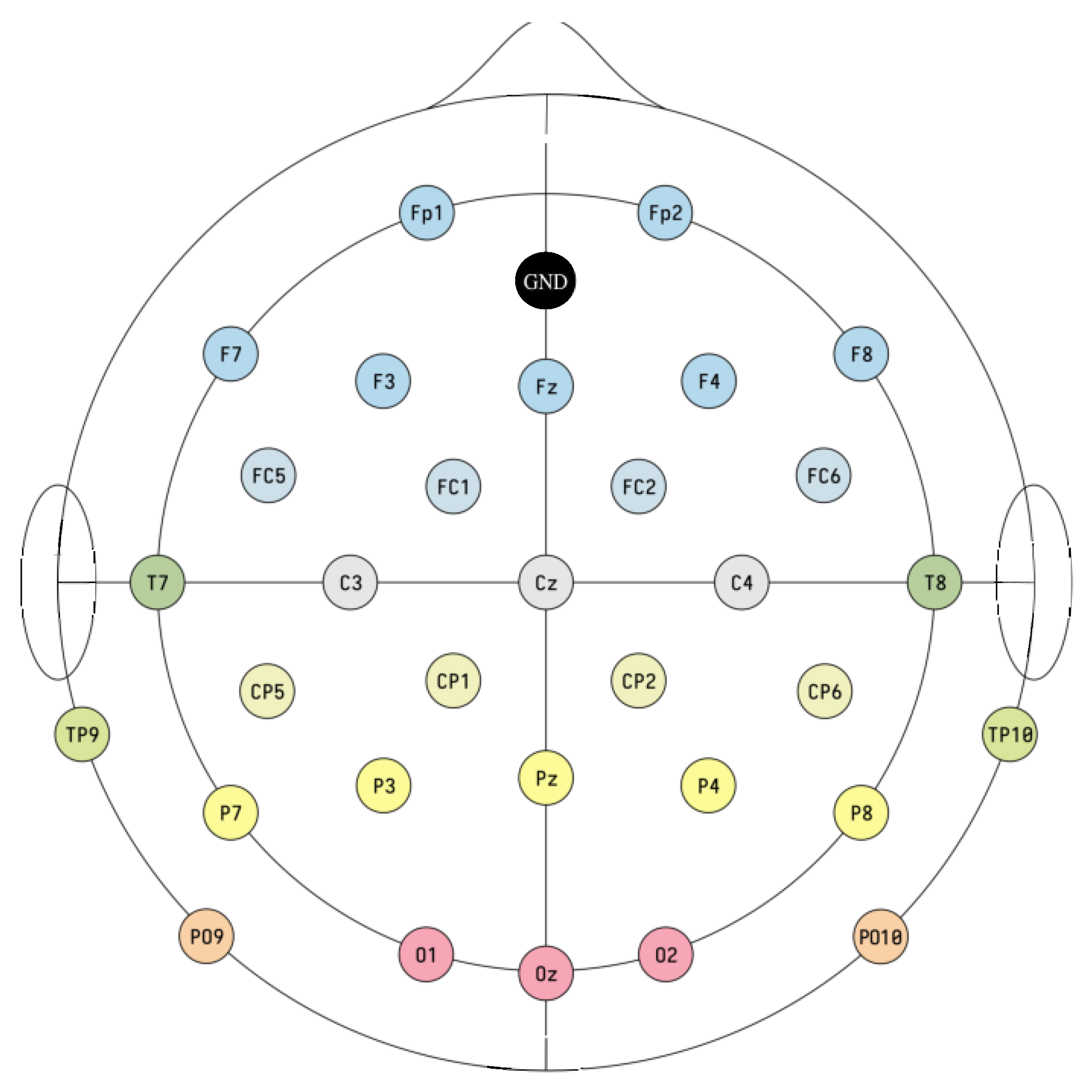
2.1. Data Acquisition
2.2. Data Preprocessing
3. Functional Connectivity from EEG Signals
3.1. Phase-Based Connectivity
Hilbert Filter
3.2. Channel Synchronization by Pearson’s Circular Correlation
4. Diagnosing Dyslexia by Outlier Detection
4.1. Outlier Detection Based on Self-Organizing Maps
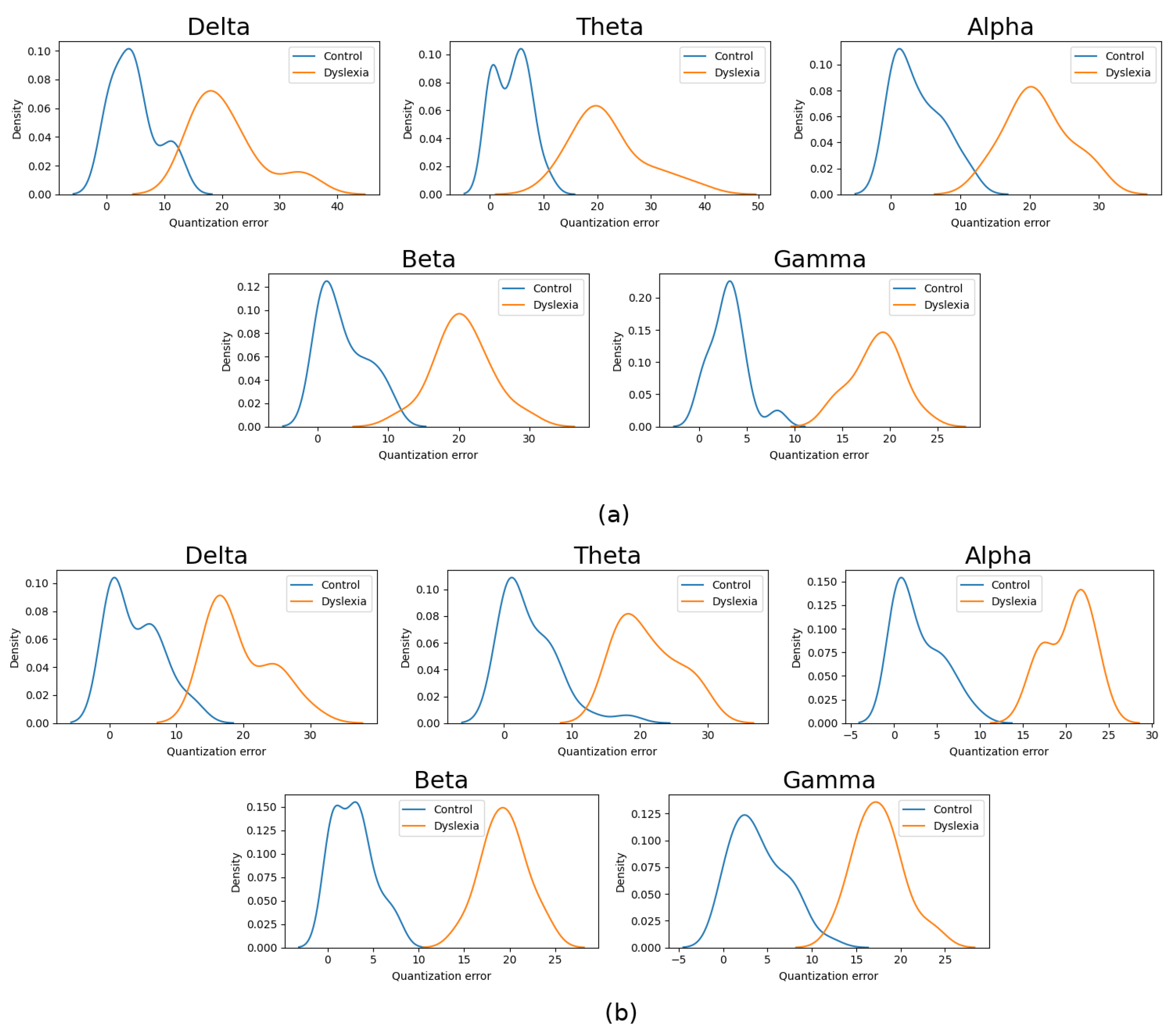
4.1.1. Band Relevance Using Quantization Error Distribution
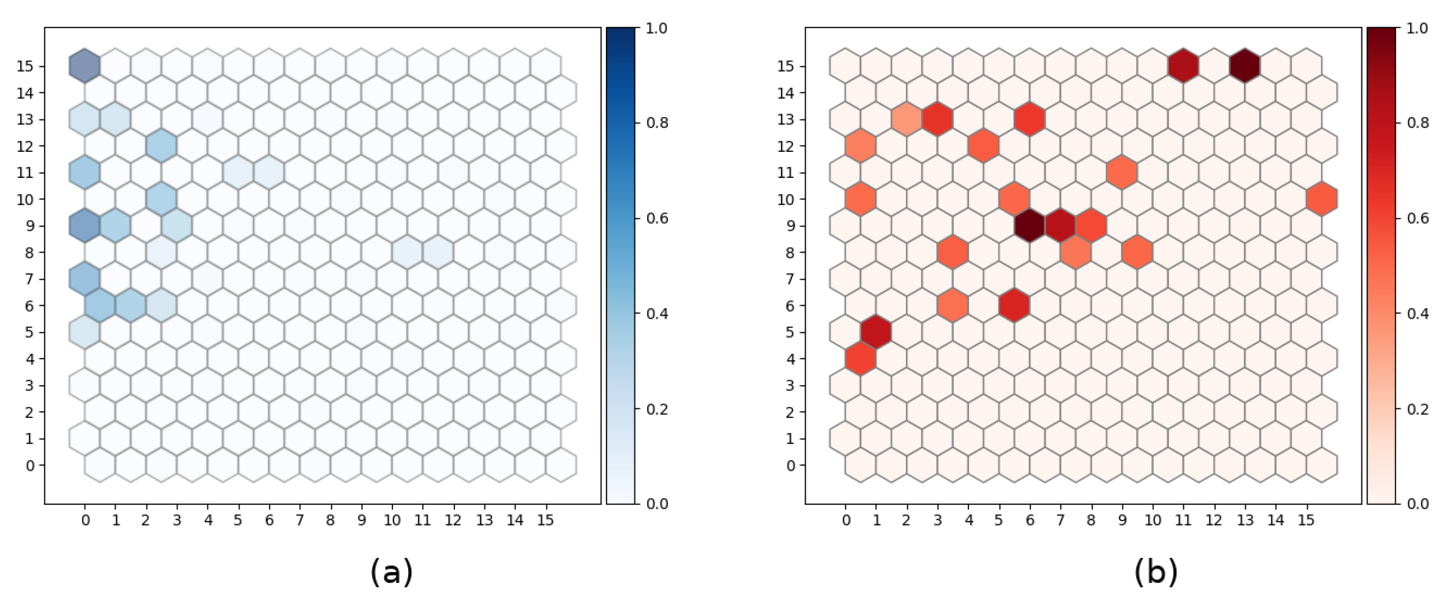
4.1.2. Uncertainly in SOM Units Activation
4.2. Bayesian Anomaly Detection for SOM
5. Results
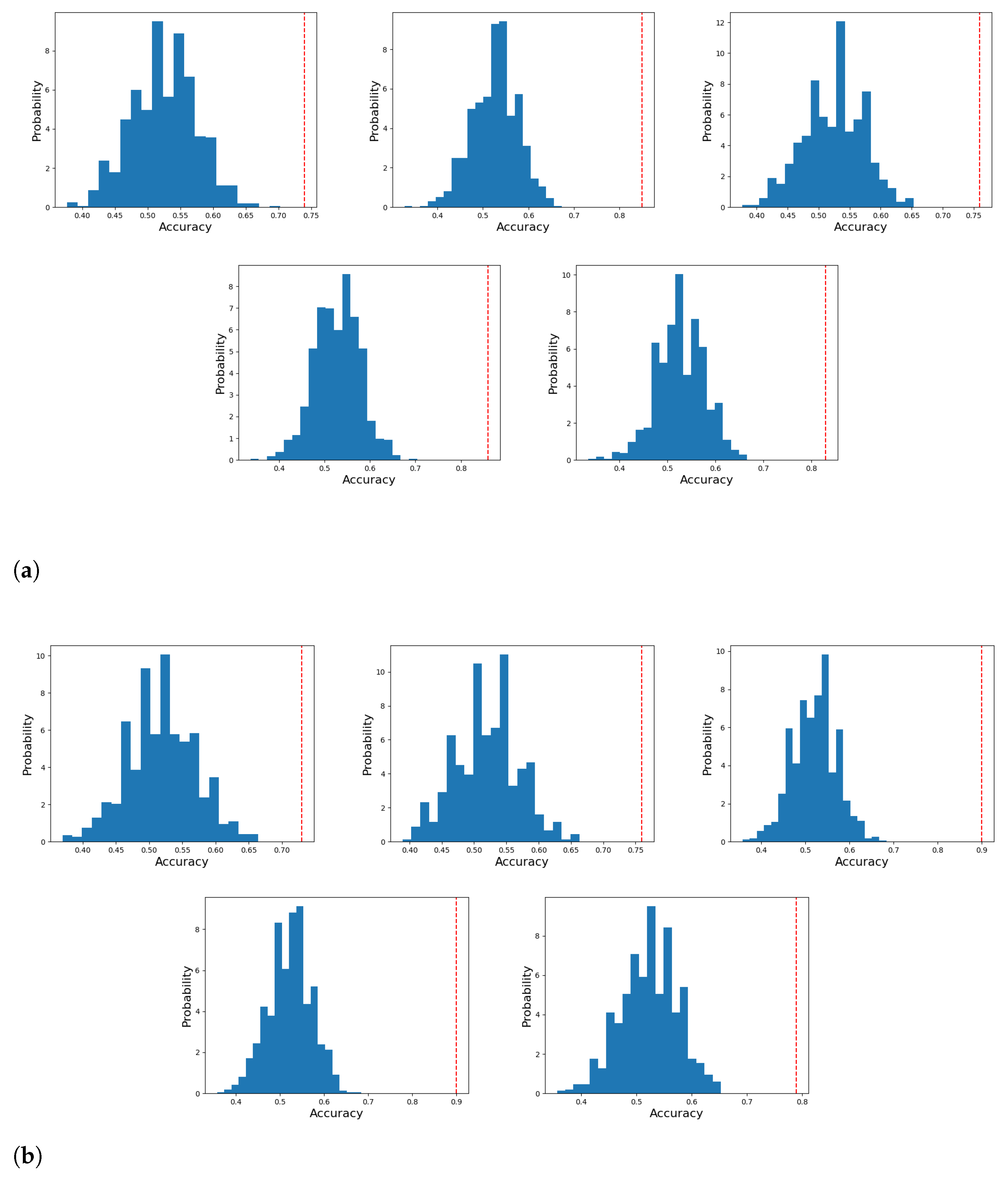
Statistical Significance
6. Discussion
7. Conclusions
Author Contributions
Funding
Institutional Review Board Statement
Informed Consent Statement
Acknowledgments
Conflicts of Interest
Abbreviations
| EEG | Electroencephalography |
| DD | Developmental Dyslexia |
| MEG | Magnetoencephalography |
| SNR | Signal to Noise Ratio |
| ICA | Independent Component Analysis |
| SC | Spectral Coherence |
| CFC | Cross Frequency Coupling |
| PAC | Phase Amplitude Coupling |
| LI | Language Impairment |
| SSD | Speech Sound Disorder |
| ADHD | Attention Deficit Hyperactivity Disorder |
| IIR | Infinite Impulse Response |
| FIR | Finite Impulse Response |
| HT | Hilbert Transform |
| PLV | Phase Locking Value |
| SOM | Self-Organizing Map |
| BUM | Best Matching Unit |
| ROC | Receiver Operating Curves |
| AUC | Area Under ROC Curve |
References
- Bell, M.A.; Cuevas, K. Using EEG to Study Cognitive Development: Issues and Practices. J. Cogn. Dev. 2012, 13, 281–294. [Google Scholar] [CrossRef] [Green Version]
- Mammone, N.; Bonanno, L.; Salvo, S.D.; Marino, S.; Bramanti, P.; Bramanti, A.; Morabito, F.C. Permutation Disalignment Index as an Indirect, EEG-Based, Measure of Brain Connectivity in MCI and AD Patients. Int. J. Neural Syst. 2017, 27, 1750020. [Google Scholar] [CrossRef] [PubMed]
- Mirzaei, G.; Adeli, A.; Adeli, H. Imaging and machine learning techniques for diagnosis of Alzheimer’s disease. Rev. Neurosci. 2016, 27, 857–870. [Google Scholar] [CrossRef]
- Gálvez, G.; Recuero, M.; Canuet, L.; Del-Pozo, F. Short-Term Effects of Binaural Beats on EEG Power, Functional Connectivity, Cognition, Gait and Anxiety in Parkinson’s Disease. Int. J. Neural Syst. 2018, 28, 1750055. [Google Scholar] [CrossRef]
- Sushkova, O.S.; Morozov, A.A.; Gabova, A.V.; Karabanov, A.V.; Illarioshkin, S.N. A Statistical Method for Exploratory Data Analysis Based on 2D and 3D Area under Curve Diagrams: Parkinson’s Disease Investigation. Sensors 2021, 21, 4700. [Google Scholar] [CrossRef]
- Adeli, H.; Zhou, Z.; Dadmehr, N. Analysis of EEG records in an epileptic patient using wavelet transform. J. Neurosci. Methods 2003, 123, 69–87. [Google Scholar] [CrossRef]
- Smith, S.J.M. EEG in the diagnosis, classification, and management of patients with epilepsy. J. Neurol. Neurosurg. Psychiatry 2005, 76, ii2–ii7. [Google Scholar] [CrossRef] [PubMed] [Green Version]
- Aileni, R.M.; Pasca, S.; Florescu, A. EEG-Brain Activity Monitoring and Predictive Analysis of Signals Using Artificial Neural Networks. Sensors 2020, 20, 3346. [Google Scholar] [CrossRef] [PubMed]
- Li, Y.; Tong, S.; Liu, D.; Gai, Y.; Wang, X.; Wang, J.; Qiu, Y.; Zhu, Y. Abnormal EEG complexity in patients with schizophrenia and depression. Clin. Neurophysiol. 2008, 119, 1232–1241. [Google Scholar] [CrossRef]
- Peterson, R.; Pennington, B. Developmental Dyslexia. Lancet 2012, 379, 1997–2007. [Google Scholar] [CrossRef] [Green Version]
- Thompson, P.A.; Hulme, C.; Nash, H.M.; Gooch, D.; Hayiou-Thomas, E.; Snowling, M.J. Developmental dyslexia: Predicting individual risk. J. Child Psychol. Psychiatry 2015, 56, 976–987. [Google Scholar] [CrossRef] [Green Version]
- Braun, U.; Muldoon, S.; Bassett, D. On Human Brain Networks in Health and Disease. eLS 2015, 1–9. [Google Scholar] [CrossRef]
- Munilla, J.; Ortiz, A.; Górriz, J.M.; Ramírez, J. Construction and Analysis of Weighted Brain Networks from SICE for the Study of Alzheimer’s Disease. Front. Neuroinform. 2017, 11, 19. [Google Scholar] [CrossRef] [PubMed]
- Ortiz, A.; Munilla, J.; Górriz, J.M.; Ramírez, J. Ensembles of Deep Learning Architectures for the Early Diagnosis of the Alzheimer’s Disease. Int. J. Neural Syst. 2016, 26, 1650025. [Google Scholar] [CrossRef] [PubMed]
- Popering, L.V.; Tahmassebi, A.; Meyer-Baese, U.; Dyrba, M.; Munilla, J.; Ortiz, A.; Meyer-Baese, A. Identifying the diffusion source of dementia spreading in structural brain networks. In Medical Imaging 2021: Biomedical Applications in Molecular, Structural, and Functional Imaging; Gimi, B.S., Krol, A., Eds.; International Society for Optics and Photonics, SPIE: Cardiff, UK, 2021; Volume 11600, pp. 58–63. [Google Scholar]
- Chaturvedi, M.; Bogaarts, J.G.; Kozak (Cozac), V.V.; Hatz, F.; Gschwandtner, U.; Meyer, A.; Fuhr, P.; Roth, V. Phase lag index and spectral power as QEEG features for identification of patients with mild cognitive impairment in Parkinson’s disease. Clin. Neurophysiol. 2019, 130, 1937–1944. [Google Scholar] [CrossRef]
- Hata, M.; Kazui, H.; Tanaka, T.; Ishii, R.; Canuet, L.; Pascual-Marqui, R.D.; Aoki, Y.; Ikeda, S.; Kanemoto, H.; Yoshiyama, K.; et al. Functional connectivity assessed by resting state EEG correlates with cognitive decline of Alzheimer’s disease—An eLORETA study. Clin. Neurophysiol. 2016, 127, 1269–1278. [Google Scholar] [CrossRef] [Green Version]
- Huang, H.; Zhang, J.; Zhu, L.; Tang, J.; Lin, G.; Kong, W.; Lei, X.; Zhu, L. EEG-Based Sleep Staging Analysis with Functional Connectivity. Sensors 2021, 21, 1988. [Google Scholar] [CrossRef]
- Daianu, M.; Jahanshad, N.; Nir, T.; Toga, A.; Jack, C.; Weiner, M.; Thompson, P. Breakdown of Brain Connectivity Between Normal Aging and Alzheimer’s Disease: A Structural k -Core Network Analysis. Brain Connect. 2013, 3, 407–422. [Google Scholar] [CrossRef] [Green Version]
- Romeo, R.R.; Segaran, J.; Leonard, J.A.; Robinson, S.T.; West, M.R.; Mackey, A.P.; Yendiki, A.; Rowe, M.L.; Gabrieli, J.D. Language Exposure Relates to Structural Neural Connectivity in Childhood. J. Neurosci. 2018, 38, 7870–7877. [Google Scholar] [CrossRef] [PubMed] [Green Version]
- Cohen, M.X. Analyzing Neural Time Series Data: Theory and Practice; MIT Press: Cambridge, MA, USA, 2014. [Google Scholar]
- Molinaro, N.; Lizarazu, M.; Lallier, M.; Bourguignon, M.; Carreiras, M. Out-of-synchrony speech entrainment in developmental dyslexia. Hum. Brain Mapp. 2016, 37, 2767–2783. [Google Scholar] [CrossRef]
- Flanagan, S.; Goswami, U. The role of phase synchronisation between low frequency amplitude modulations in child phonology and morphology speech tasks. J. Acoust. Soc. Am. 2018, 143, 1366–1375. [Google Scholar] [CrossRef]
- Di Liberto, G.; Peter, V.; Kalashnikova, M.; Goswami, U.; Burnham, D.; Lalor, E. Atypical cortical entrainment to speech in the right hemisphere underpins phonemic deficits in dyslexia. NeuroImage 2018, 175, 70–79. [Google Scholar] [CrossRef] [PubMed]
- Power, A.J.; Mead, N.; Barnes, L.; Goswami, U. Neural entrainment to rhythmic speech in children with developmental dyslexia. Front. Hum. Neurosci. 2013, 7, 777. [Google Scholar] [CrossRef] [PubMed] [Green Version]
- Gibbon, S.; Attaheri, A.; Choisdealbha, Á.N.; Rocha, S.; Brusini, P.; Mead, N.; Boutris, P.; Olawole-Scott, H.; Ahmed, H.; Flanagan, S.; et al. Machine learning accurately classifies neural responses to rhythmic speech vs. non-speech from 8-week-old infant EEG. Brain Lang. 2021, 220, 104968. [Google Scholar] [CrossRef]
- Perera, H.; Shiratuddin, M.F.; Wong, K.W.; Fullarton, K. EEG signal analysis of writing and typing between adults with dyslexia and normal controls. Int. J. Interact. Multimed. Artif. Intell. 2018, 5, 62. [Google Scholar] [CrossRef] [Green Version]
- Ortiz, A.; López, P.; Luque, J.L.; Martínez-Murcia, F.J.; Aquino-Britez, D.; Ortega, J. An anomaly detection approach for dyslexia diagnosis using EEG signals. In Proceedings of the International Work—Conference on the Interplay between Natural and Artificial Computation, Almería, Spain, 3–7 June 2019; Springer: London, UK, 2019; pp. 369–378. [Google Scholar]
- Martínez-Murcia, F.J.; Ortiz, A.; Morales-Ortega, R.; López, P.; Luque, J.L.; Castillo-Barnes, D.; Segovia, F.; Illan, I.A.; Ortega, J.; Ramirez, J.; et al. Periodogram connectivity of EEG signals for the detection of dyslexia. In Proceedings of the International Work—Conference on the Interplay between Natural and Artificial Computation, Almería, Spain, 3–7 June 2019; Springer: London, UK, 2019; pp. 350–359. [Google Scholar]
- Martinez-Murcia, F.J.; Ortiz, A.; Gorriz, J.M.; Ramirez, J.; Lopez-Abarejo, P.J.; Lopez-Zamora, M.; Luque, J.L. EEG Connectivity Analysis Using Denoising Autoencoders for the Detection of Dyslexia. Int. J. Neural Syst. 2020, 30, 2050037. [Google Scholar] [CrossRef] [PubMed]
- Riaz, F.; Hassan, A.; Rehman, S.; Niazi, I.K.; Dremstrup, K. EMD-Based Temporal and Spectral Features for the Classification of EEG Signals Using Supervised Learning. IEEE Trans. Neural Syst. Rehabil. Eng. 2016, 24, 28–35. [Google Scholar] [CrossRef]
- Boashash, B. Chapter 16—Time-Frequency Methodologies in Neurosciences. In Time-Frequency Signal Analysis and Processing, 2nd ed.; Academic Press: Oxford, UK, 2016; pp. 915–966. [Google Scholar]
- Unde, S.A.; Shriram, R. Coherence Analysis of EEG Signal Using Power Spectral Density. In Proceedings of the 2014 Fourth International Conference on Communication Systems and Network Technologies, Bhopal, India, 7–9 April 2014; pp. 871–874. [Google Scholar]
- Munia, T.T.K.; Aviyente, S. Time-Frequency Based Phase-Amplitude Coupling Measure For Neuronal Oscillations. Sci. Rep. 2019, 9, 1–15. [Google Scholar] [CrossRef] [Green Version]
- Giménez, A.; Luque, J.L.; López-Zamora, M.; Fernández-Navas, M. A self-report questionnaire on reading-writing difficulties for adults. [Autoinforme de Trastornos Lectores para AdultoS (ATLAS)]. An. Psicol./Ann. Psychol. 2015, 31, 109–119. [Google Scholar] [CrossRef] [Green Version]
- De Vos, A.; Vanvooren, S.; Vanderauwera, J.; Ghesquière, P.; Wouters, J. A longitudinal study investigating neural processing of speech envelope modulation rates in children with (a family risk for) dyslexia. Cortex 2017, 93, 206–219. [Google Scholar] [CrossRef]
- Li, R.; Principe, J.C. Blinking Artifact Removal in Cognitive EEG Data Using ICA. In Proceedings of the 2006 International Conference of the IEEE Engineering in Medicine and Biology Society, New York, NY, USA, 30 August–3 September 2006; pp. 5273–5276. [Google Scholar]
- Robertson, D.; Dowling, J. Design and responses of Butterworth and critically damped digital filters. J. Electromyogr. Kinesiol. Off. J. Int. Soc. Electrophysiol. Kinesiol. 2004, 13, 569–573. [Google Scholar] [CrossRef]
- Jiménez-Bravo, M.; Marrero, V.; Benítez-Burraco, A. An oscillopathic approach to developmental dyslexia: From genes to speech processing. Behav. Brain Res. 2017, 329, 84–95. [Google Scholar] [CrossRef] [PubMed]
- Mormann, F.; Lehnertz, K.; David, P.; Elger, C.E. Mean phase coherence as a measure for phase synchronization and its application to the EEG of epilepsy patients. Phys. D Nonlinear Phenom. 2000, 144, 358–369. [Google Scholar] [CrossRef]
- Fraiwan, L.; Lweesy, K.; Khasawneh, N.; Wenz, H.; Dickhaus, H. Automated sleep stage identification system based on time–frequency analysis of a single EEG channel and random forest classifier. Comput. Methods Programs Biomed. 2012, 108, 10–19. [Google Scholar] [CrossRef]
- Huang, N.E.; Shen, Z.; Long, S.R.; Wu, M.C.; Shih, H.H.; Zheng, Q.; Yen, N.C.; Tung, C.C.; Liu, H.H. The empirical mode decomposition and the Hilbert spectrum for nonlinear and non-stationary time series analysis. Proc. R. Soc. London Ser. A Math. Phys. Eng. Sci. 1998, 454, 903–995. [Google Scholar] [CrossRef]
- Virtanen, P.; Gommers, R.; Oliphant, T.E.; Haberland, M.; Reddy, T.; Cournapeau, D.; Burovski, E.; Peterson, P.; Weckesser, W.; Bright, J.; et al. SciPy 1.0: Fundamental algorithms for scientific computing in Python. Nat. Methods 2020, 17, 261–272. [Google Scholar] [CrossRef] [Green Version]
- Lachaux, J.P.; Rodriguez, E.; Martinerie, J.; Varela, F.J. Measuring phase synchrony in brain signals. Hum. Brain Mapp. 1999, 8, 194–208. [Google Scholar] [CrossRef] [Green Version]
- Burgess, A. On the Interpretation of Synchronization in EEG Hyperscanning Studies: A Cautionary Note. Front. Hum. Neurosci. 2013, 7, 881. [Google Scholar] [CrossRef] [PubMed] [Green Version]
- Rothmaler, K.; Ivanova, G. Circular Correlation Coefficients versus the Phase-Locking-Value. Biomed. Tech. Biomed. Eng. 2013, 58. [Google Scholar] [CrossRef]
- Jammalamadaka, S.R.; SenGupta, A. Topics in Circular Statistics, 1st ed.; World Scientific: Singapore, 2016. [Google Scholar] [CrossRef]
- Golub, T.R.; Slonim, D.K.; Tamayo, P.; Huard, C.; Gaasenbeek, M.; Mesirov, J.P.; Coller, H.; Loh, M.L.; Downing, J.R.; Caligiuri, M.A.; et al. Molecular classification of cancer: Class discovery and class prediction by gene expression monitoring. Science 1999, 286, 531–537. [Google Scholar] [CrossRef] [Green Version]
- Lawrence, S.; Giles, C.L.; Tsoi, A.C.; Back, A.D. Face recognition: A convolutional neural-network approach. IEEE Trans. Neural Netw. 1997, 8, 98–113. [Google Scholar] [CrossRef] [PubMed] [Green Version]
- Betti, A.; Tucci, M.; Crisostomi, E.; Piazzi, A.; Barmada, S.; Thomopulos, D. Fault Prediction and Early-Detection in Large PV Power Plants Based on Self-Organizing Maps. Sensors 2021, 21, 1687. [Google Scholar] [CrossRef] [PubMed]
- Cai, W.; Zhao, D.; Zhang, M.; Xu, Y.; Li, Z. Improved Self-Organizing Map-Based Unsupervised Learning Algorithm for Sitting Posture Recognition System. Sensors 2021, 21, 6246. [Google Scholar] [CrossRef]
- Vesanto, J.; Alhoniemi, E. Clustering of the self-organizing map. IEEE Trans. Neural Netw. 2000, 11, 586–600. [Google Scholar] [CrossRef] [PubMed]
- De la Hoz, E.; De La Hoz, E.; Ortiz, A.; Ortega, J.; Prieto, B. PCA filtering and probabilistic SOM for network intrusion detection. Neurocomputing 2015, 164, 71–81. [Google Scholar] [CrossRef]
- Vettigli, G. MiniSom: Minimalistic and NumPy-Based Implementation of the Self Organizing Map. Available online: https://github.com/JustGlowing/minisom/ (accessed on 10 October 2021).
- Kohonen, T. Self-Organizing Maps; Springer: London, UK, 2001. [Google Scholar]
- Kullback, S.; Leibler, R.A. On Information and Sufficiency. Ann. Math. Stat. 1951, 22, 79–86. [Google Scholar] [CrossRef]
- John, G.; Langley, P. Estimating Continuous Distributions in Bayesian Classifiers. arXiv 2013, arXiv:1302.4964. [Google Scholar]
- Bhattacharyya, S.; Khasnobish, A.; Konar, A.; Tibarewala, D.N.; Nagar, A.K. Performance analysis of left/right hand movement classification from EEG signal by intelligent algorithms. In Proceedings of the 2011 IEEE Symposium on Computational Intelligence, Cognitive Algorithms, Mind, and Brain (CCMB), Paris, France, 11–15 April 2011; pp. 1–8. [Google Scholar] [CrossRef]
- Čukić, M.; Stokić, M.; Simic, S.; Pokrajac, D. The successful discrimination of depression from EEG could be attributed to proper feature extraction and not to a particular classification method. Cogn. Neurodyn. 2020, 14, 443–455. [Google Scholar] [CrossRef] [Green Version]
- Siuly, S.; Wang, H.; Zhang, Y. Detection of motor imagery EEG signals employing Naïve Bayes based learning process. Measurement 2016, 86, 148–158. [Google Scholar] [CrossRef]
- Duin, R.P. Classifiers in almost empty spaces. In Proceedings of the 15th International Conference on Pattern Recognition, ICPR-2000, Barcelona, Spain, 3–7 September 2000; Volume 2, pp. 1–7. [Google Scholar]
- Pedregosa, F.; Varoquaux, G.; Gramfort, A.; Michel, V.; Thirion, B.; Grisel, O.; Blondel, M.; Prettenhofer, P.; Weiss, R.; Dubourg, V.; et al. Scikit-learn: Machine Learning in Python. J. Mach. Learn. Res. 2011, 12, 2825–2830. [Google Scholar]
- Hickok, G.; Poeppel, D. The Cortical Organization of Speech Processing. Nat. Rev. Neurosci. 2007, 8, 393–402. [Google Scholar] [CrossRef]
- Virtala, P.; Talola, S.; Partanen, E.; Kujala, T. Poor neural and perceptual phoneme discrimination during acoustic variation in dyslexia. Sci. Rep. 2020, 10, 1–11. [Google Scholar] [CrossRef]
- Giehl, J.; Noury, N.; Siegel, M. Dissociating harmonic and non-harmonic phase-amplitude coupling in the human brain. NeuroImage 2021, 227, 117648. [Google Scholar] [CrossRef] [PubMed]
- Colling, L.J.; Noble, H.L.; Goswami, U. Neural entrainment and sensorimotor synchronization to the beat in children with developmental dyslexia: An EEG study. Front. Neurosci. 2017, 11, 360. [Google Scholar] [CrossRef] [PubMed]
- Tamboer, P.; Vorst, H.; Ghebreab, S.; Scholte, H. Machine learning and dyslexia: Classification of individual structural neuro-imaging scans of students with and without dyslexia. Neuroimage Clin. 2016, 11, 508–514. [Google Scholar] [CrossRef] [PubMed] [Green Version]
- Dimitriadis, S.I.; Simos, P.G.; Fletcher, J.M.; Papanicolaou, A.C. Aberrant resting-state functional brain networks in dyslexia: Symbolic mutual information analysis of neuromagnetic signals. Int. J. Psychophysiol. 2018, 126, 20–29. [Google Scholar] [CrossRef] [PubMed]


| Group | Male/Female | Mean Age (Months) | Observations |
|---|---|---|---|
| Control | 17/15 | No reported reading or spelling difficulties | |
| Dyslexia | 7/9 | Formal diagnosis by a clinician expert |
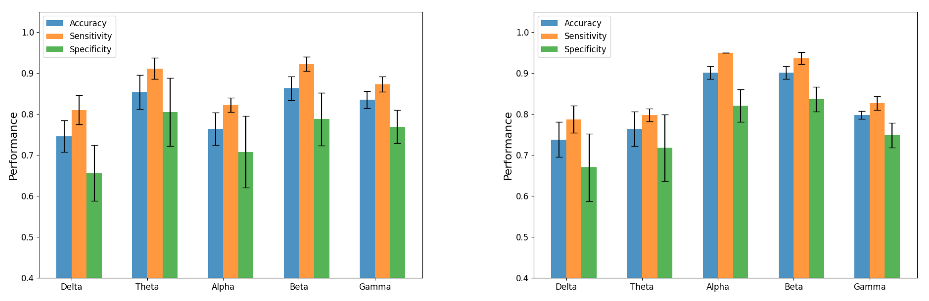
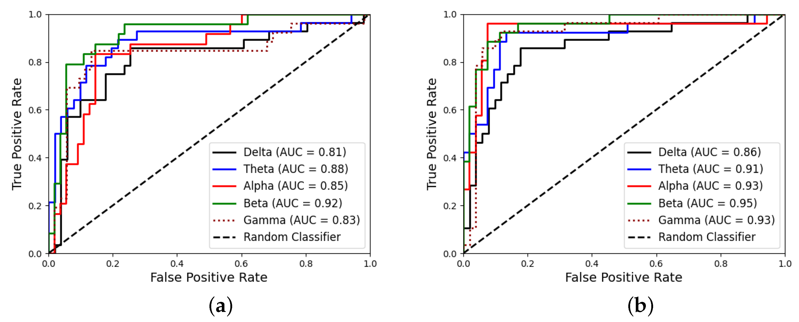
| Stimulus | Band | Accuracy | Sensitivity | Specificity | AUC |
|---|---|---|---|---|---|
| 4.8 Hz | Delta | 0.74 ± 0.03 | 0.81 ± 0.03 | 0.65 ± 0.06 | 0.81 ± 0.05 |
| Theta | 0.85 ± 0.04 | 0.91 ± 0.03 | 0.80 ± 0.08 | 0.88 ± 0.05 | |
| Alpha | 0.76 ± 0.04 | 0.82 ± 0.02 | 0.70 ± 0.09 | 0.85 ± 0.08 | |
| Beta | 0.86 ± 0.03 | 0.92 ± 0.02 | 0.78 ± 0.06 | 0.92 ± 0.08 | |
| Gamma | 0.83 ± 0.02 | 0.87 ± 0.02 | 0.76 ± 0.04 | 0.83 ± 0.05 | |
| 16 Hz | Delta | 0.73 ± 0.04 | 0.78 ± 0.03 | 0.67 ± 0.08 | 0.86 ± 0.07 |
| Theta | 0.76 ± 0.04 | 0.79 ± 0.02 | 0.71 ± 0.08 | 0.91 ± 0.05 | |
| Alpha | 0.90 ± 0.02 | 0.93 ± 0.01 | 0.82 ± 0.04 | 0.93 ± 0.09 | |
| Beta | 0.90 ± 0.02 | 0.93 ± 0.02 | 0.86 ± 0.03 | 0.95 ± 0.09 | |
| Gamma | 0.79 ± 0.01 | 0.82 ± 0.02 | 0.74 ± 0.03 | 0.93 ± 0.10 |
| Method | Channels | Acq.Time | Accuracy | Sensitivity | Specificity | AUC |
|---|---|---|---|---|---|---|
| MRI + SVC [67] | T1-MRI | * | 0.8 ± * | 0.82 ± * | 0.78 ± * | * |
| MEG + SVC + GC [68] | 253 | 3 min | 0.63 ± 4.13 | 0.64 ± 4.01 | 0.65 ± 4.15 | * |
| MEG + SVC + GE [68] | 253 | 3 min | 0.94 ± 1.78 | 0.93 ± 1.39 | 0.93 ± 2.32 | * |
| MEG + SVC + CI [68] | 253 | 3 min | 0.80 ± 1.14 | 0.80 ± 1.41 | 0.79 ± 2.17 | * |
| MEG + SVC + wIFCG [68] | 253 | 3 min | 0.97 ± 1.89 | 0.96 ± 1.89 | 0.95 ± 1.98 | * |
| EEG + SVC [27] (Writing Task) | 32 | 1 min | 0.59 ± * | 0.64 ± * | 0.53 ± * | * |
| EEG + SVC [27] (Typing Task) | 32 | 1 min | 0.78 ± * | 0.88 ± * | 0.66 ± * | * |
| EEG + OCSVC [28] | 32 | 5 min | 0.71 ± * | 0.53 ± * | 0.78 ± * | 0.79 ± * |
| EEG + DAE [30] | 32 | 5 min | 0.56 ± * | 0.76 ± * | 0.66 ± * | 0.74 ± * |
| Proposed | 32 | 5 min | 0.90 ± 0.02 | 0.93 ± 0.02 | 0.86 ± 0.03 | 0.95 ± 0.09 |
Publisher’s Note: MDPI stays neutral with regard to jurisdictional claims in published maps and institutional affiliations. |
© 2021 by the authors. Licensee MDPI, Basel, Switzerland. This article is an open access article distributed under the terms and conditions of the Creative Commons Attribution (CC BY) license (https://creativecommons.org/licenses/by/4.0/).
Share and Cite
Formoso, M.A.; Ortiz, A.; Martinez-Murcia, F.J.; Gallego, N.; Luque, J.L. Detecting Phase-Synchrony Connectivity Anomalies in EEG Signals. Application to Dyslexia Diagnosis. Sensors 2021, 21, 7061. https://0-doi-org.brum.beds.ac.uk/10.3390/s21217061
Formoso MA, Ortiz A, Martinez-Murcia FJ, Gallego N, Luque JL. Detecting Phase-Synchrony Connectivity Anomalies in EEG Signals. Application to Dyslexia Diagnosis. Sensors. 2021; 21(21):7061. https://0-doi-org.brum.beds.ac.uk/10.3390/s21217061
Chicago/Turabian StyleFormoso, Marco A., Andrés Ortiz, Francisco J. Martinez-Murcia, Nicolás Gallego, and Juan L. Luque. 2021. "Detecting Phase-Synchrony Connectivity Anomalies in EEG Signals. Application to Dyslexia Diagnosis" Sensors 21, no. 21: 7061. https://0-doi-org.brum.beds.ac.uk/10.3390/s21217061