
Non-Singleton Type-3 Fuzzy Approach for Flowmeter Fault Detection: Experimental Study in a Gas Industry

 ,
,  , ,
, ,  , , and
Abstract
:1. Introduction
2. Literature Review
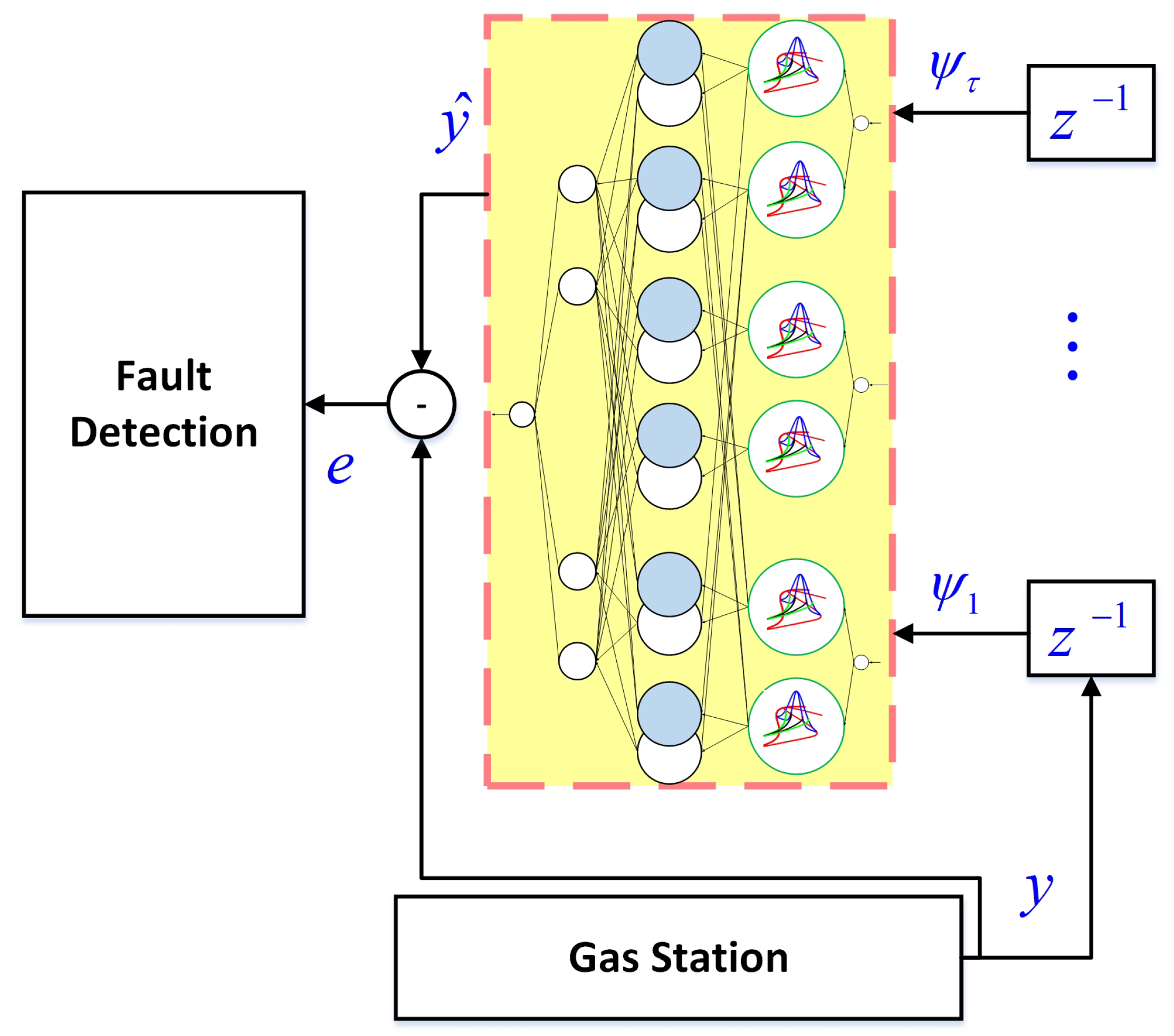
3. General View on Suggested Approach
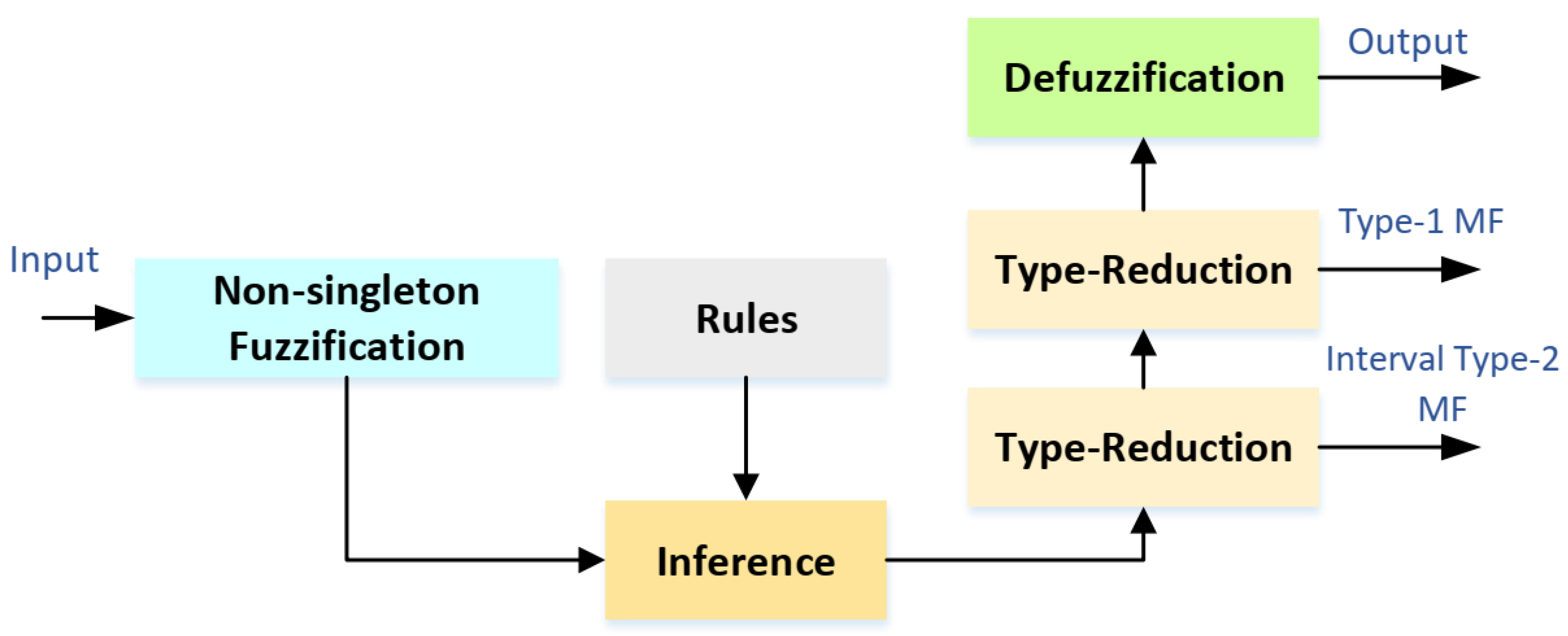
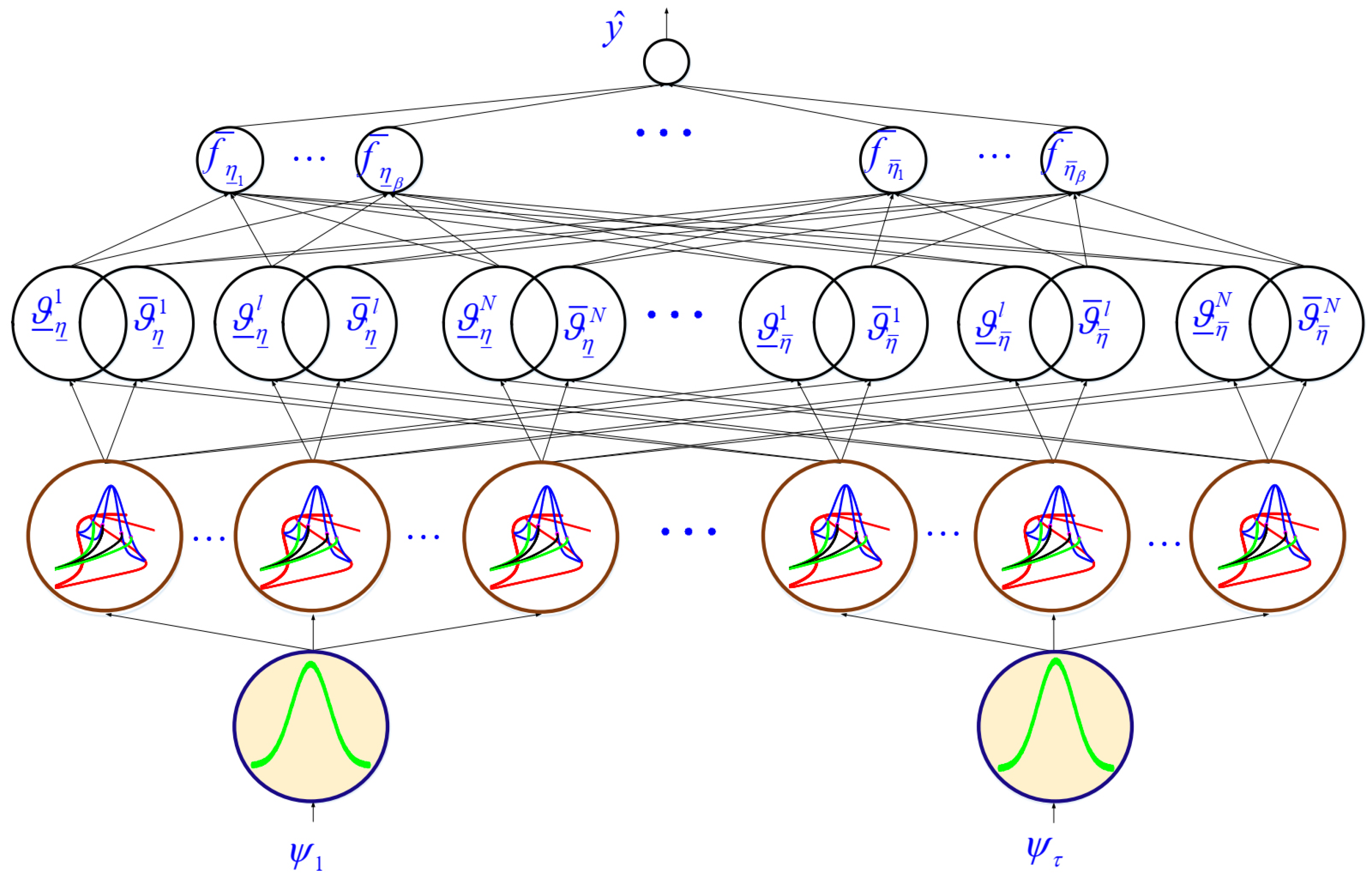
4. Non-Singleton Interval Type-3 FLS
5. Learning Algorithm
5.1. Rule Parameters
5.2. Antecedent Parameters
- (1)
- The designed NT3FLS is rewritten as:where,where, is vector of rule (consequent) parameters, is the center of MF for input , is the level of fuzzification and N is the number of MFs.
- (2)
- Initialize the vector and .
- (3)
- The sigma-points are defined as:where denotes the number of elements of vector , is covariance matrix of , is the -th column of and denotes the turning factor.
- (4)
- Compute (estimated signal) as:
- (5)
- Compute and as:whereL represents the dimension of , and is:The value of is obtained by a FLS [35].
- (6)
- and are updated as:where is
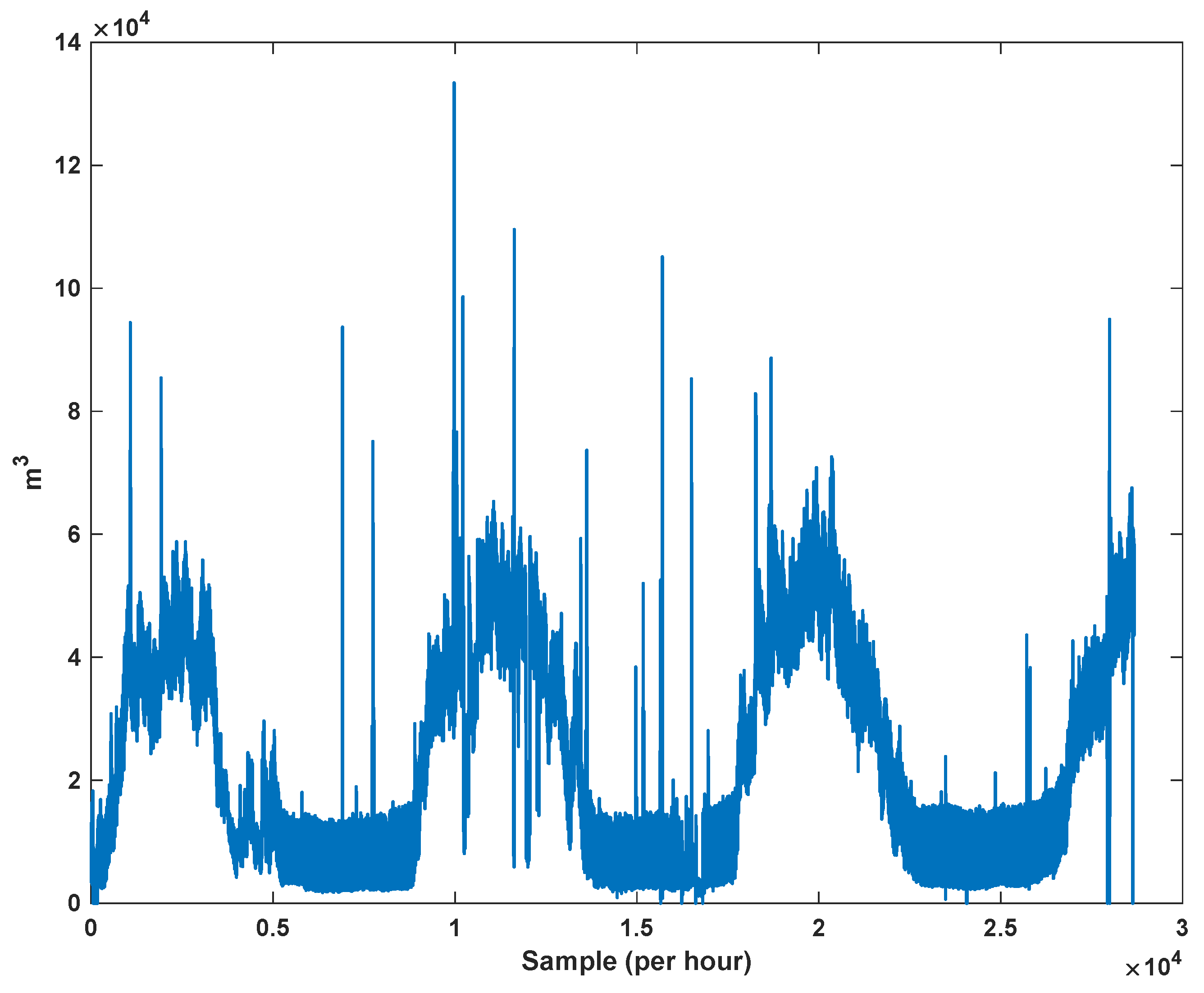
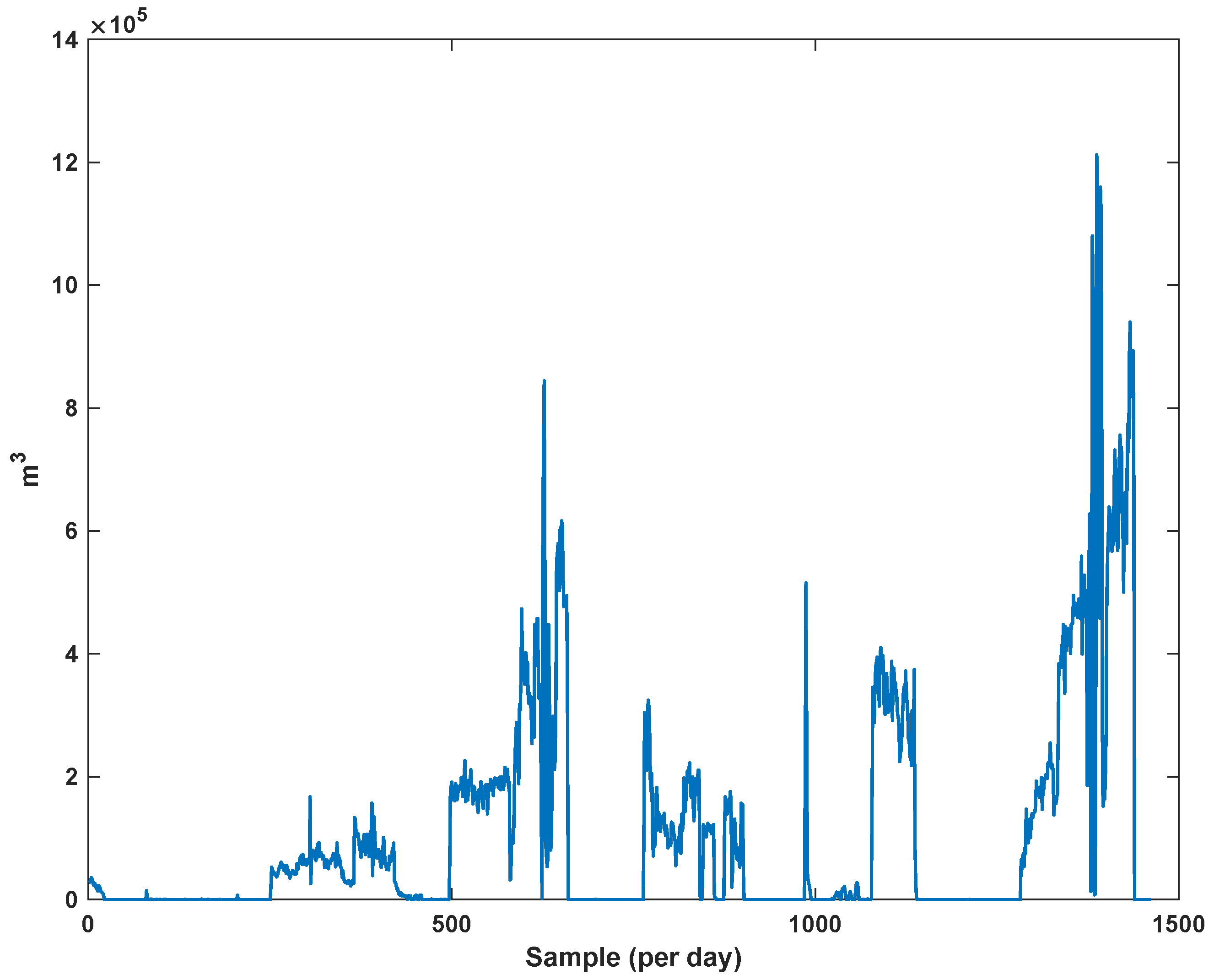
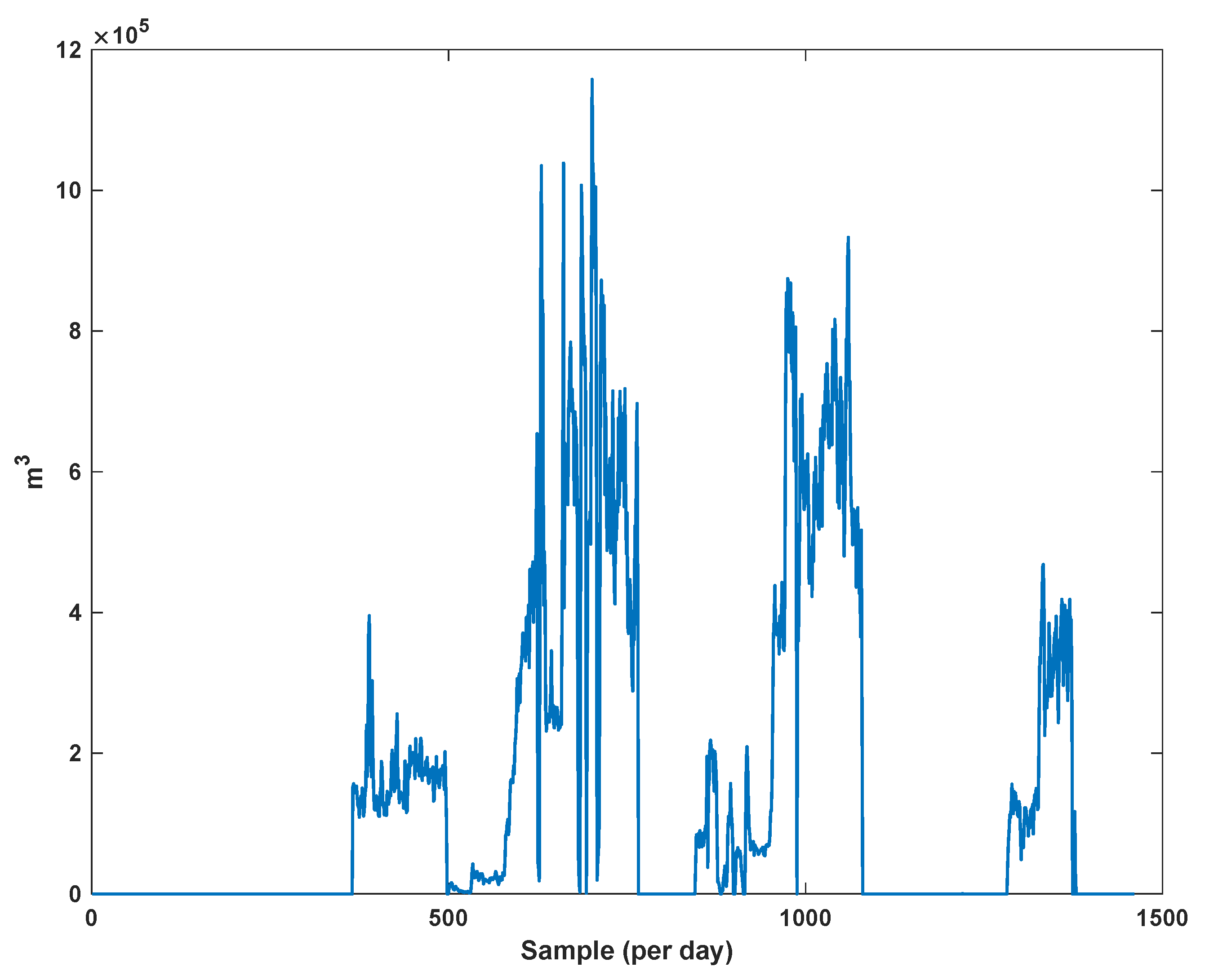
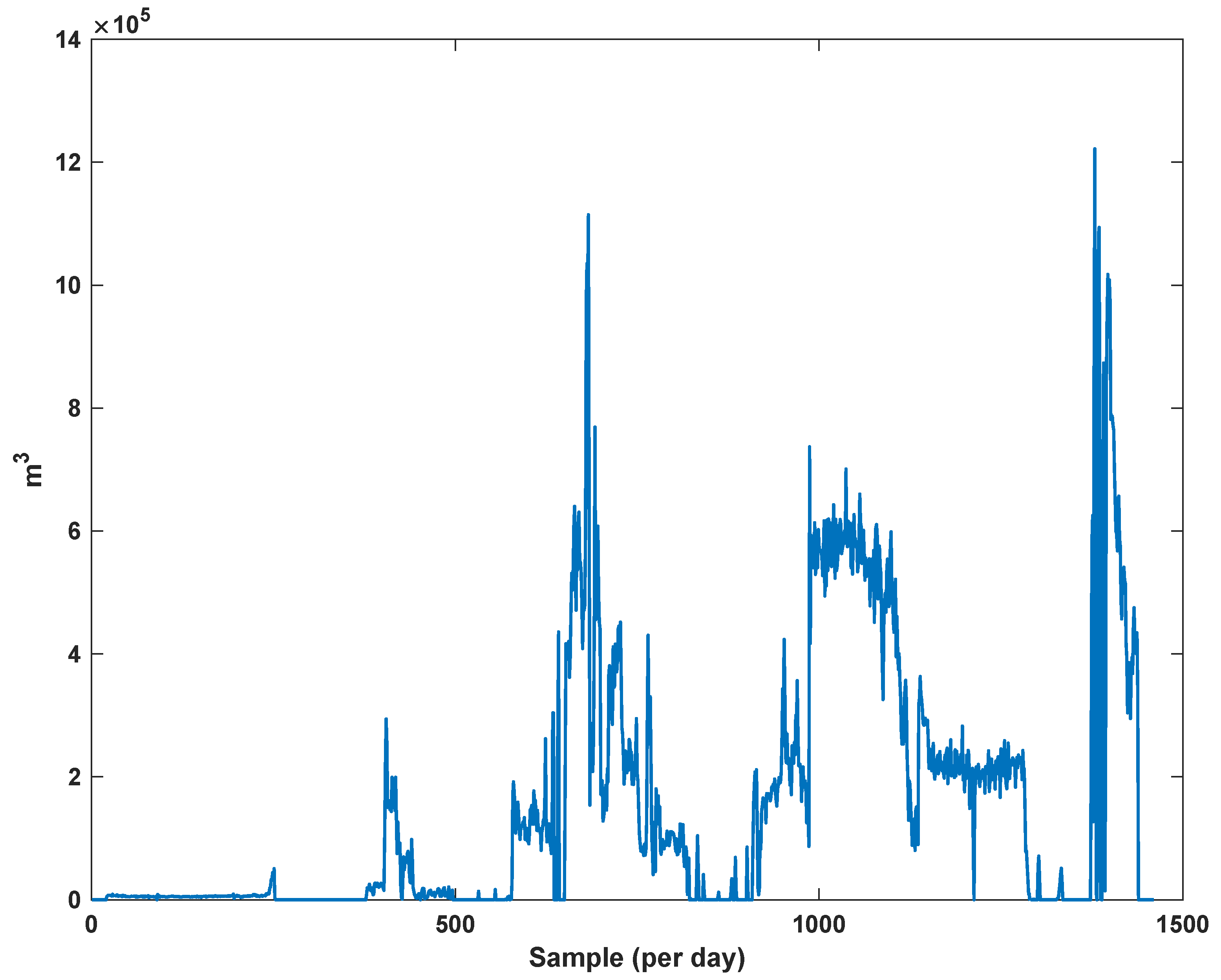
6. Data Description
7. Simulation
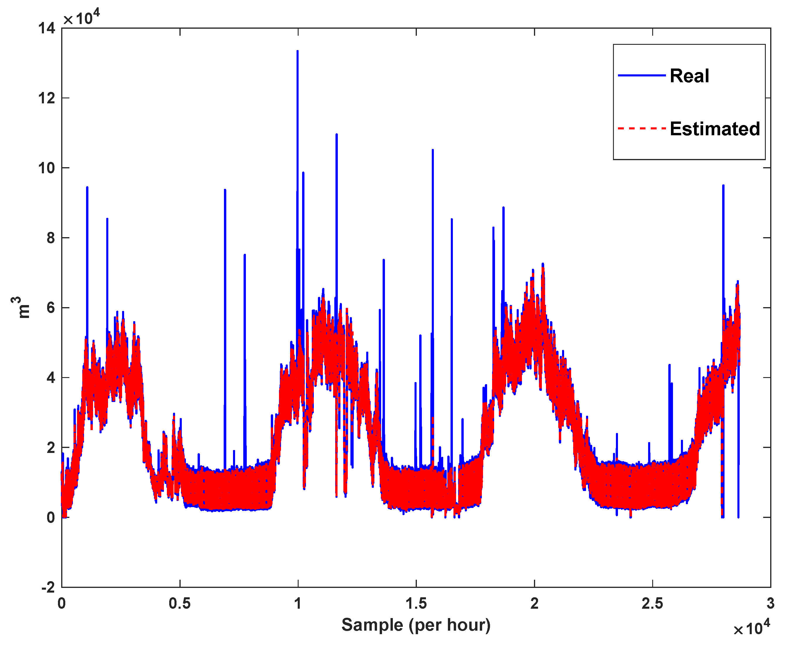
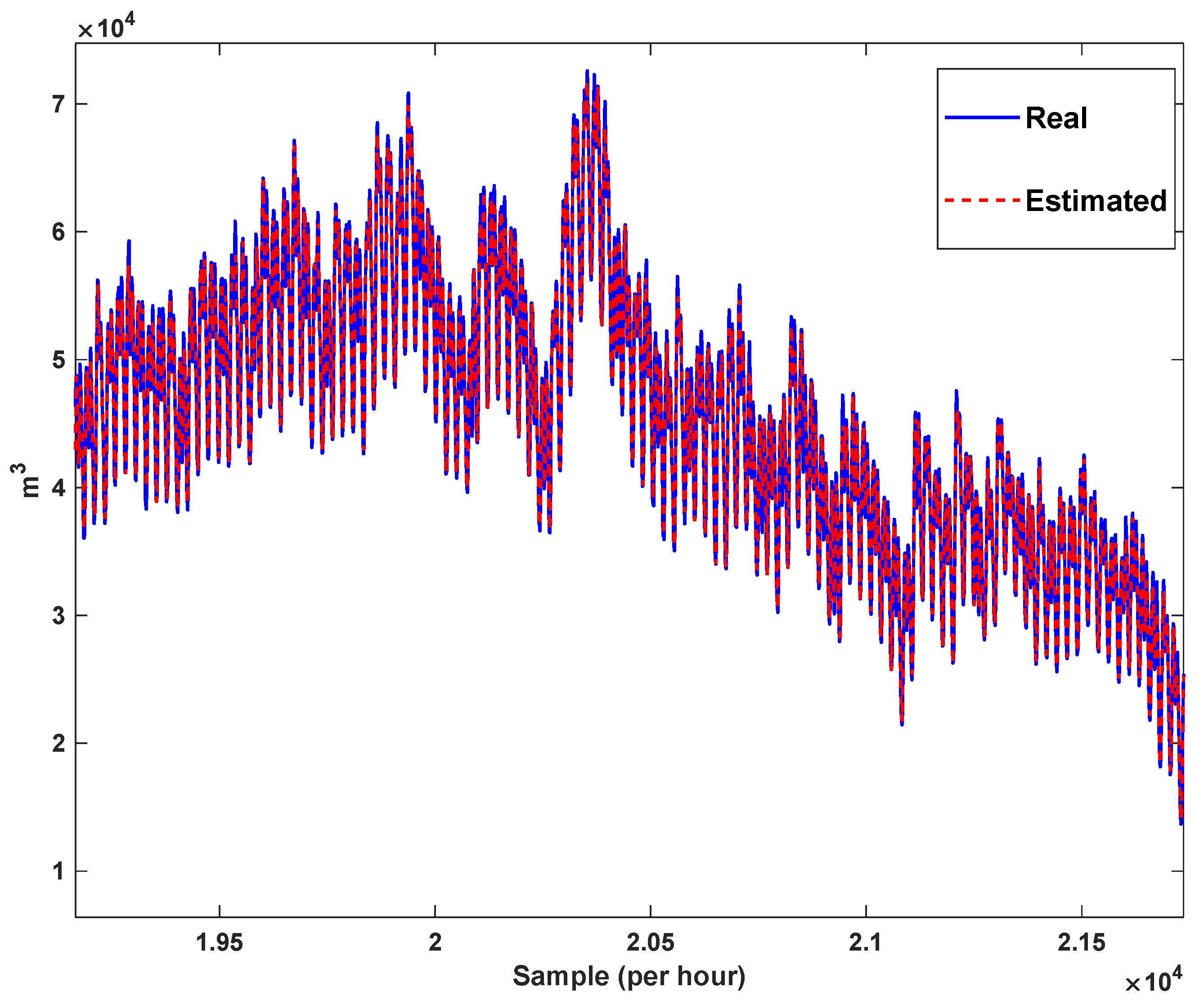
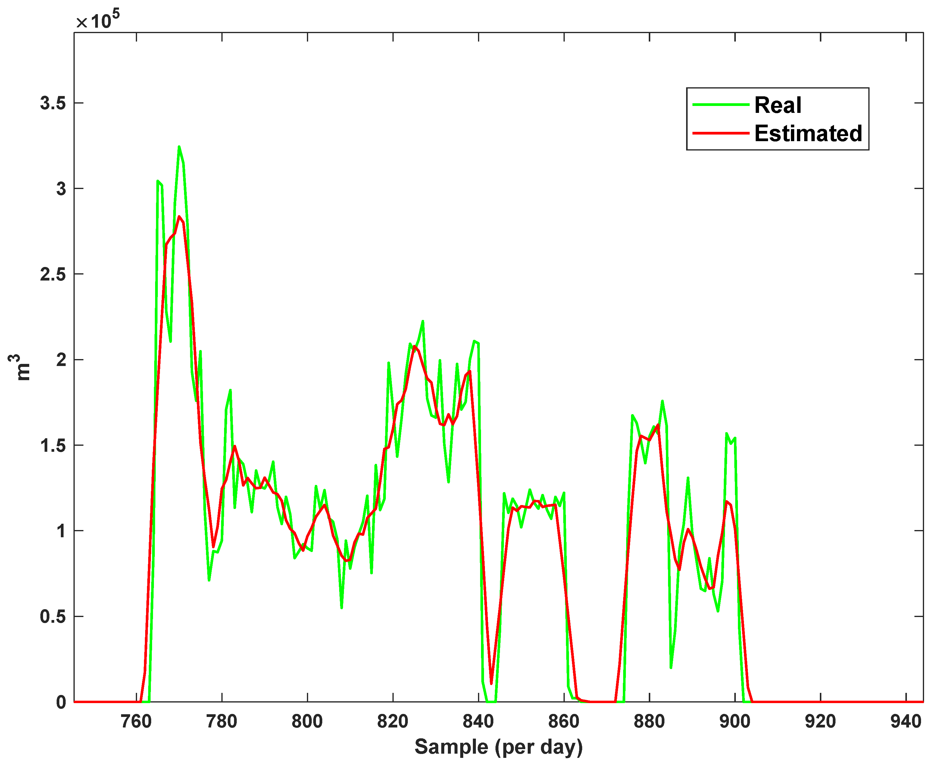
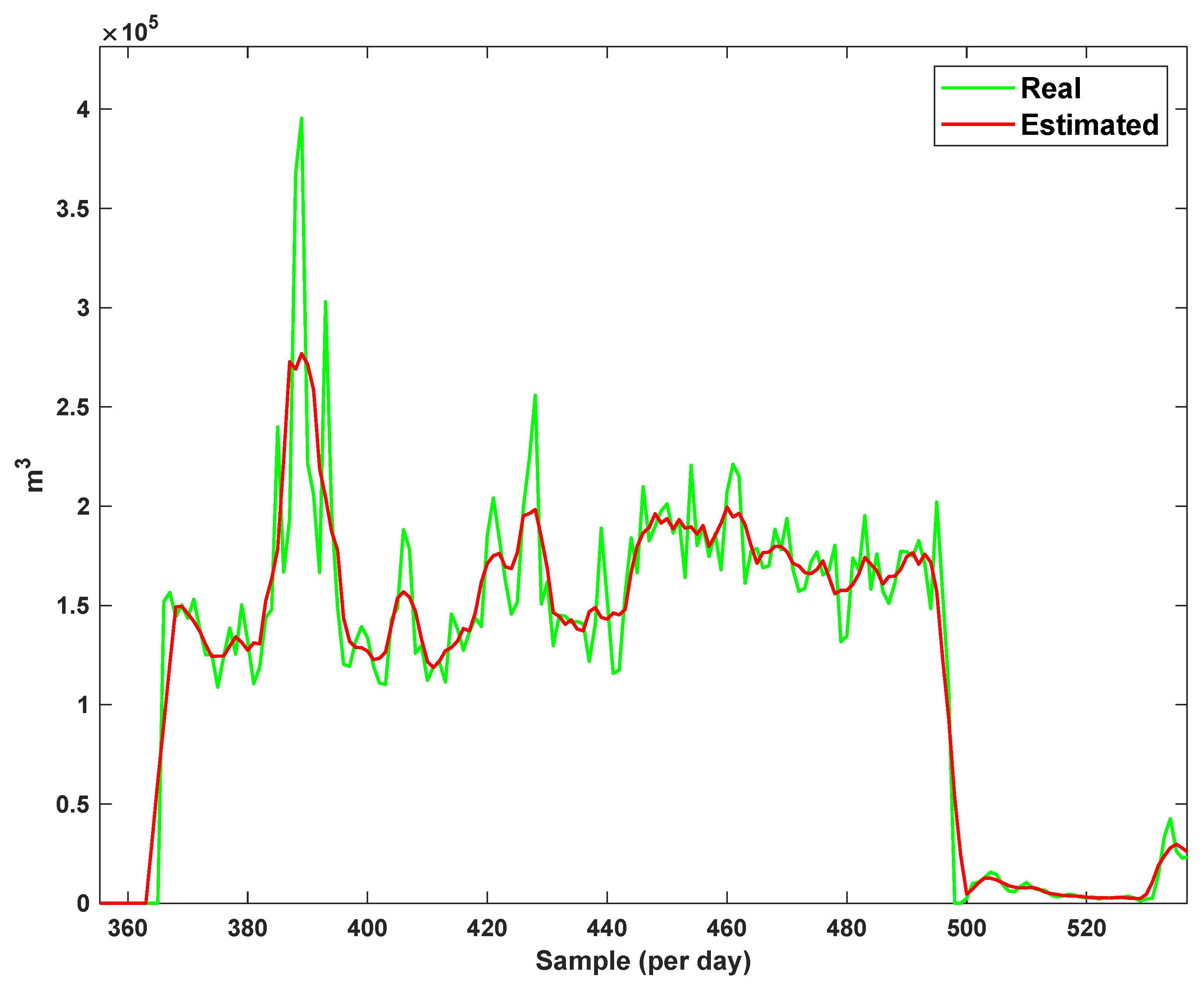
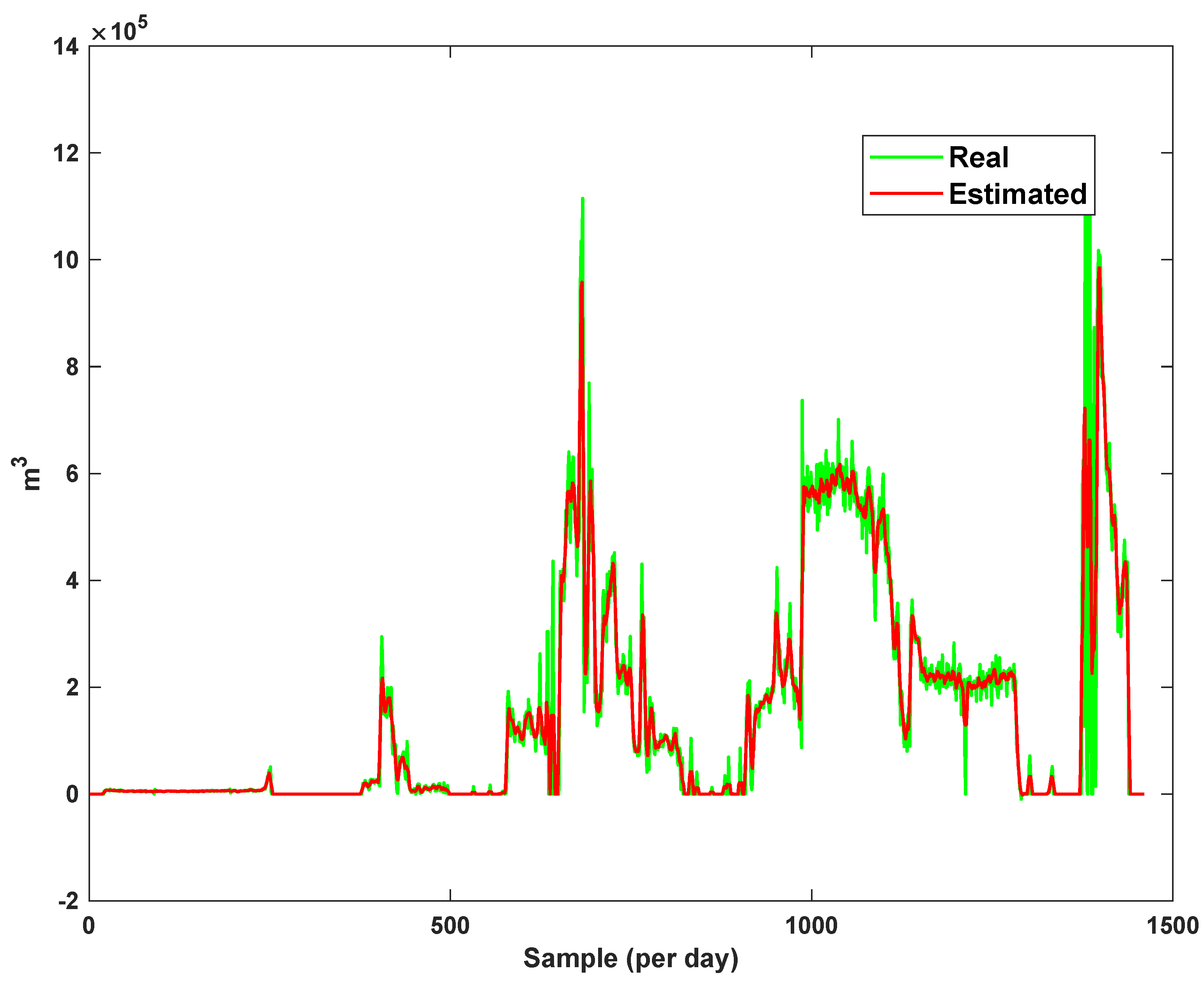
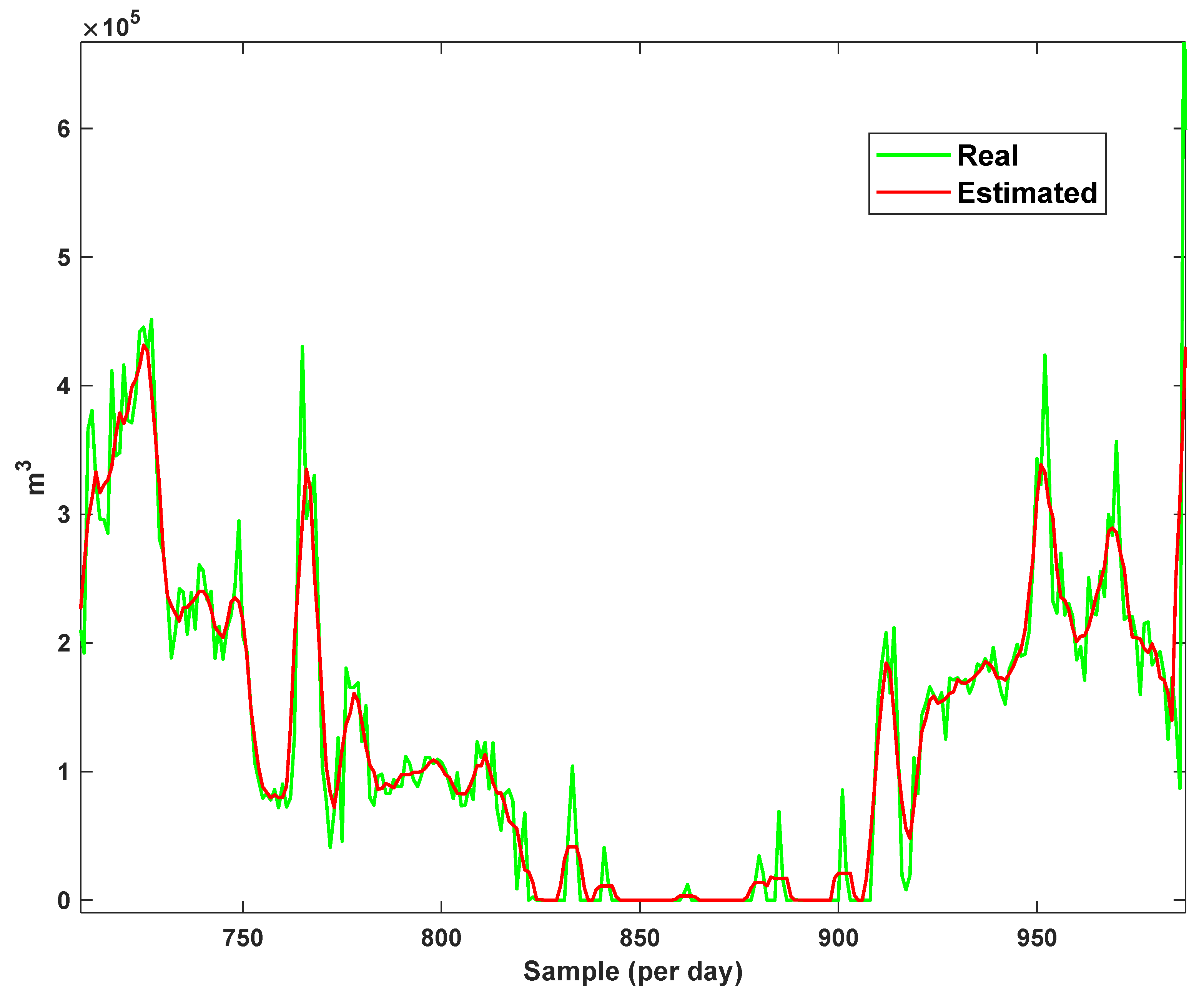
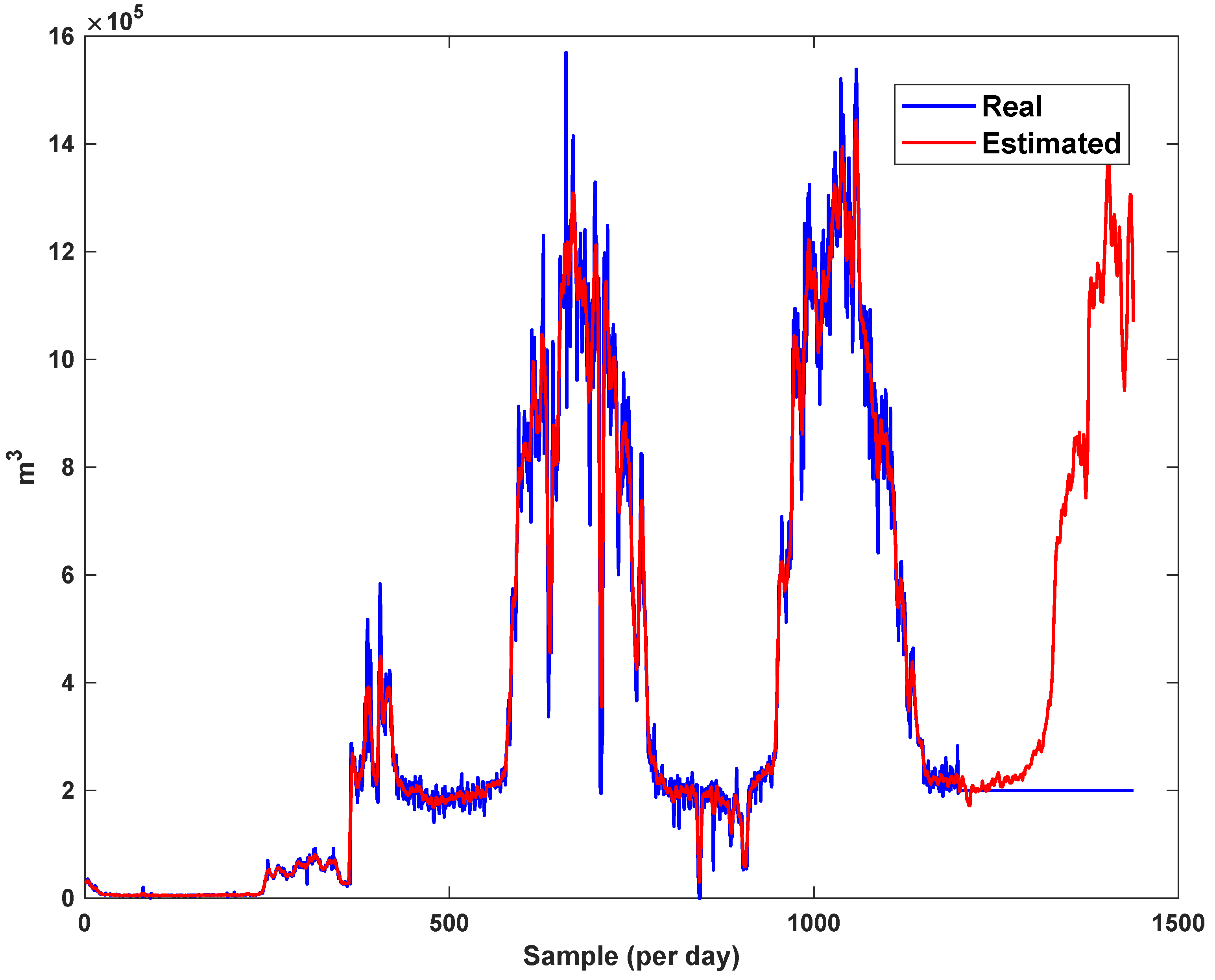
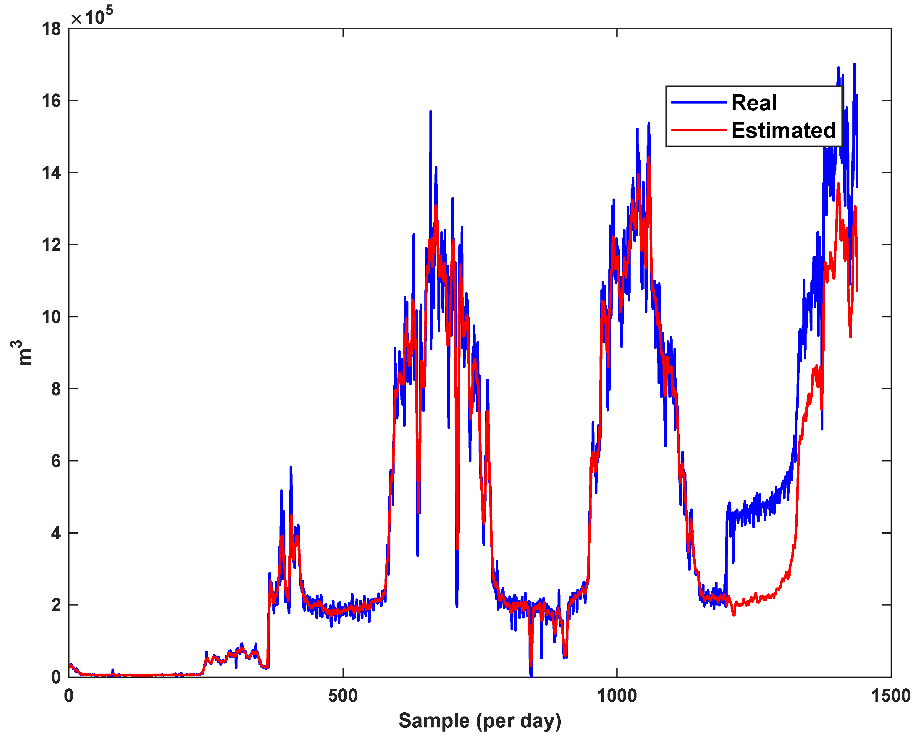
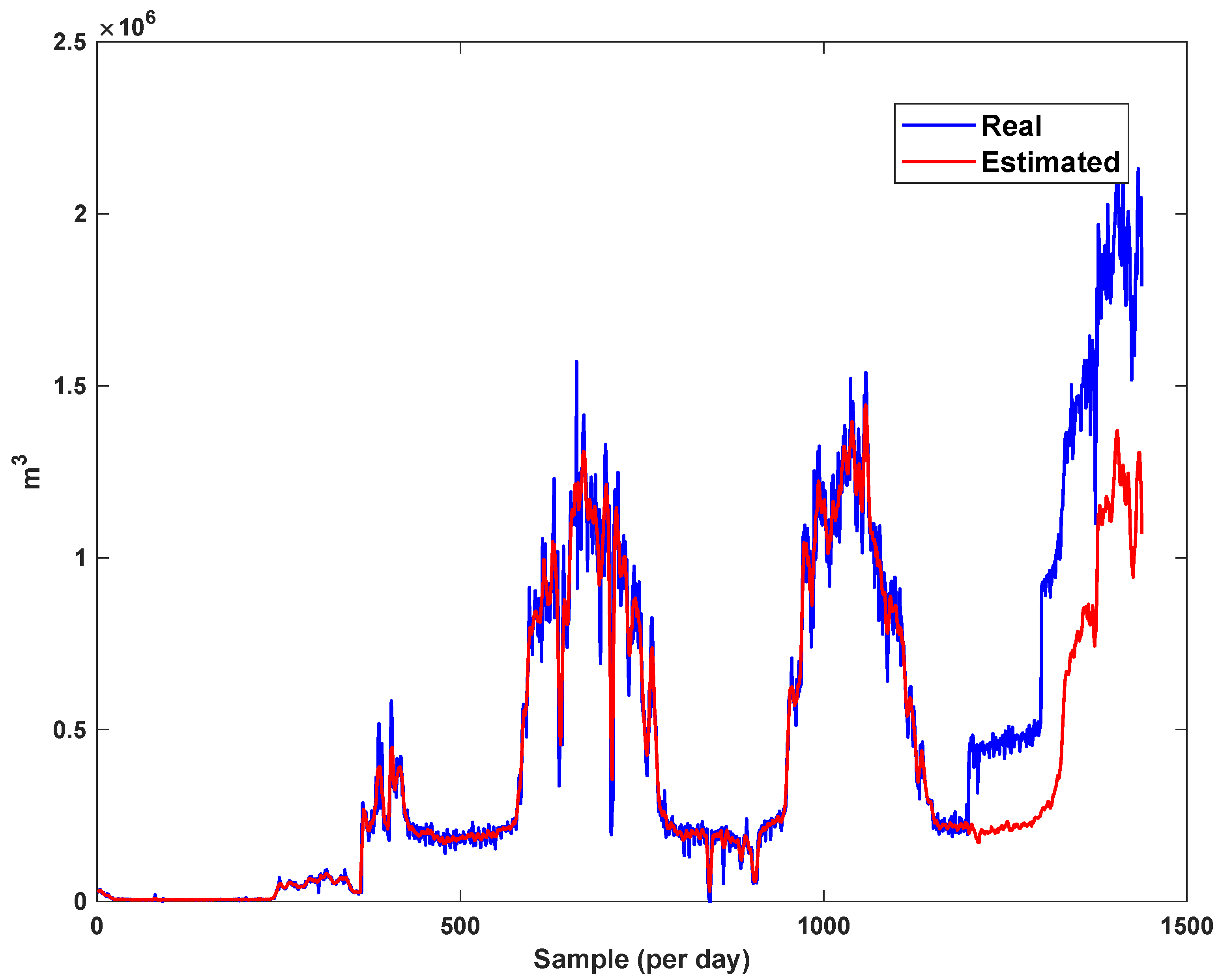
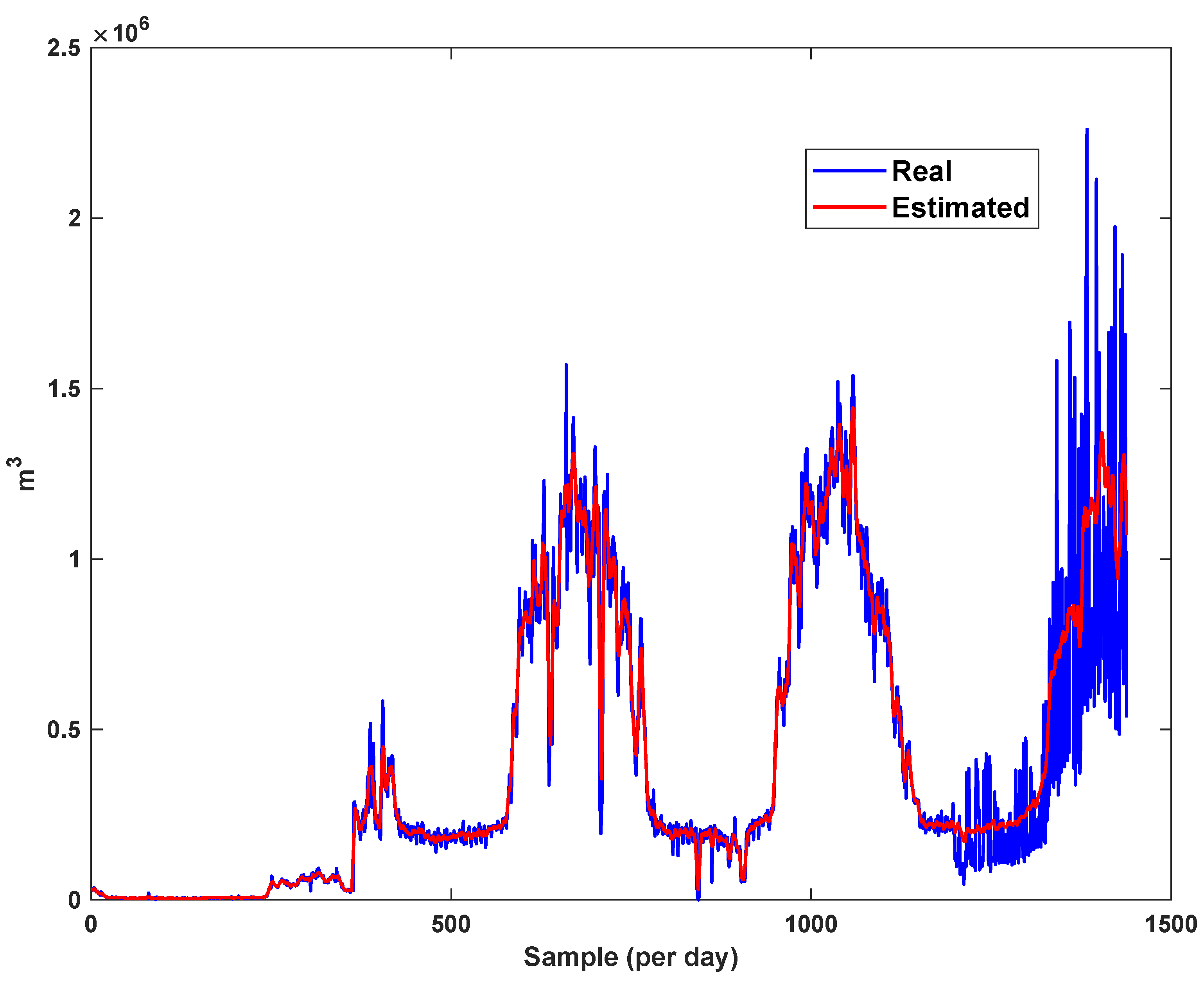
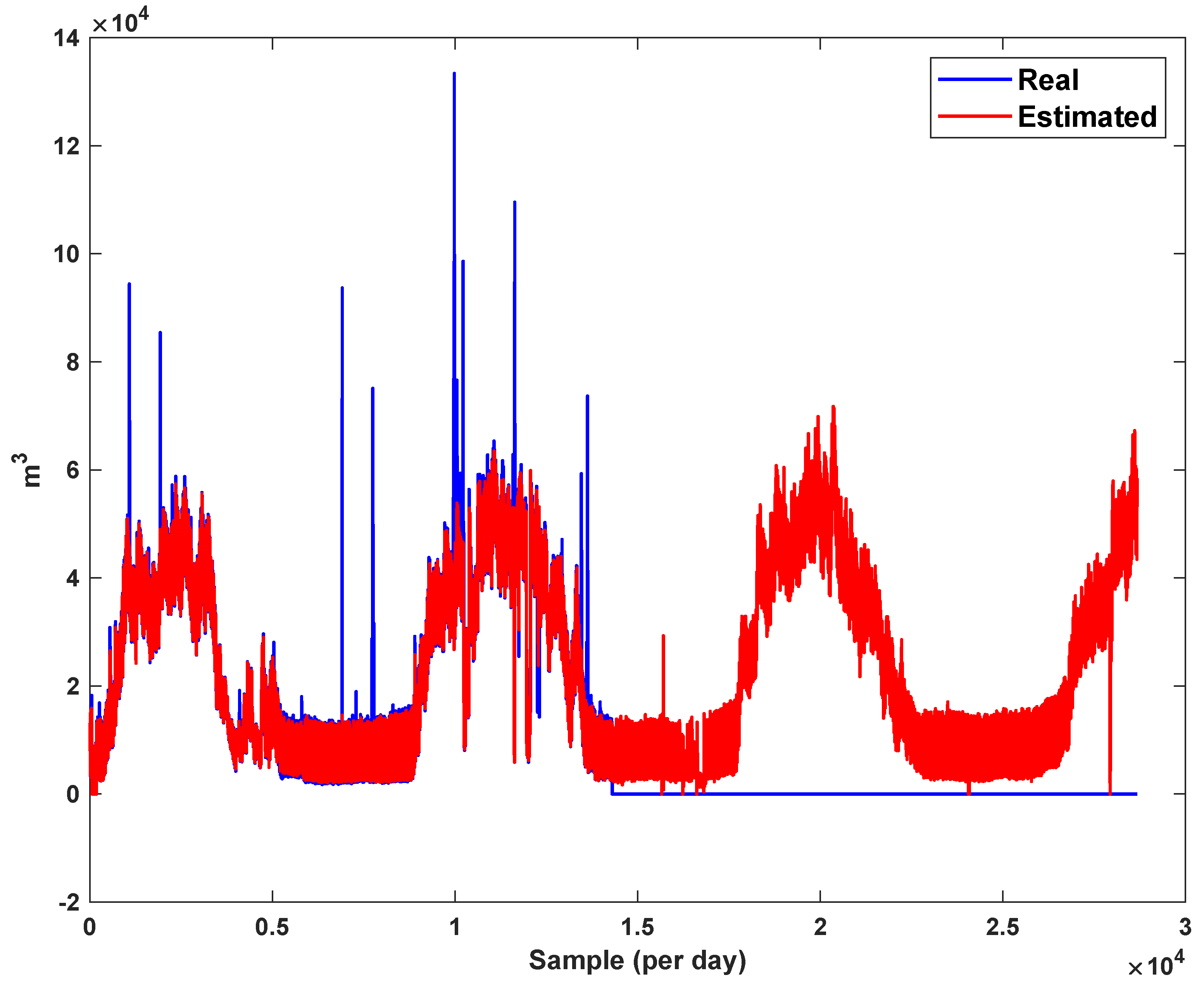
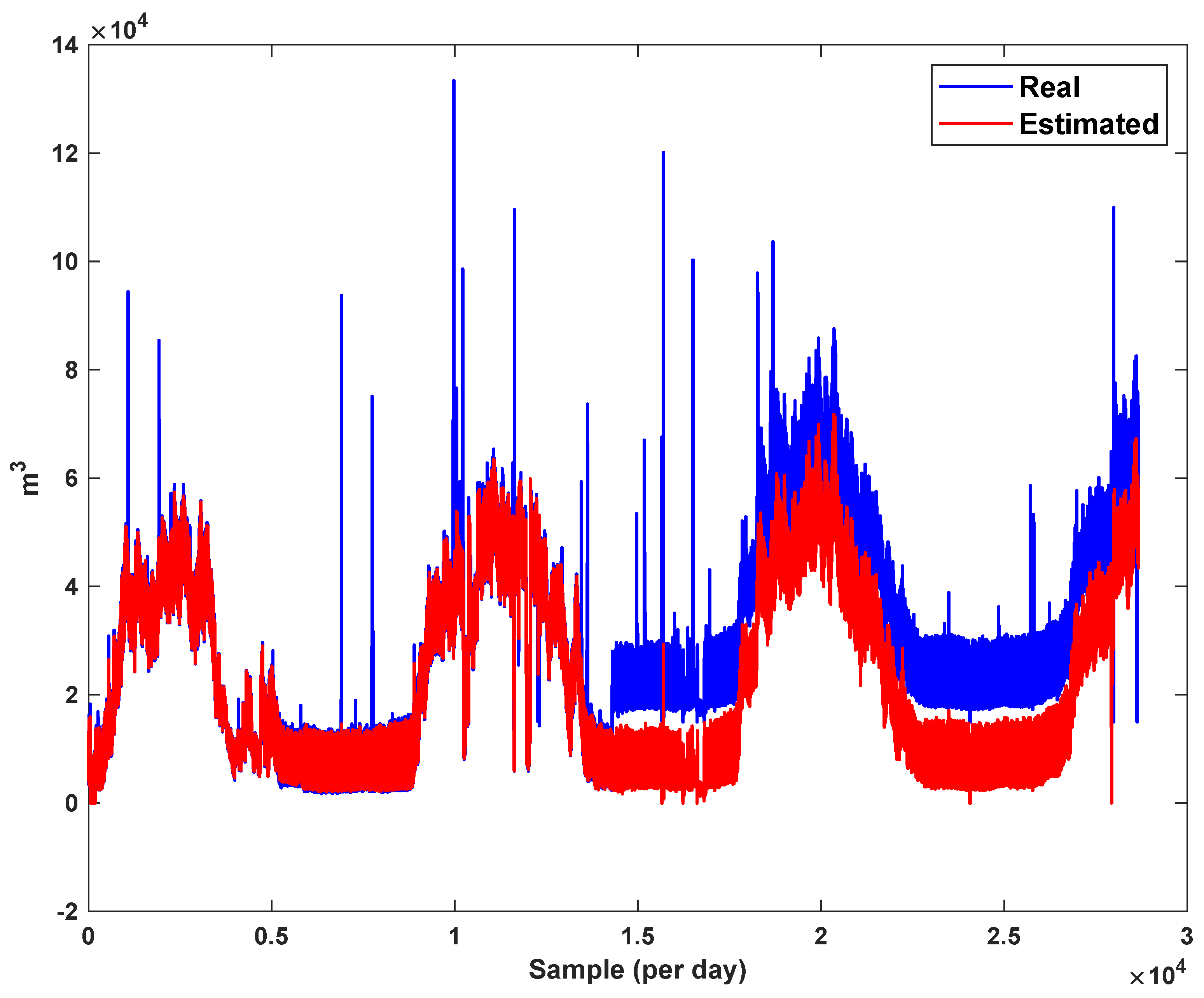
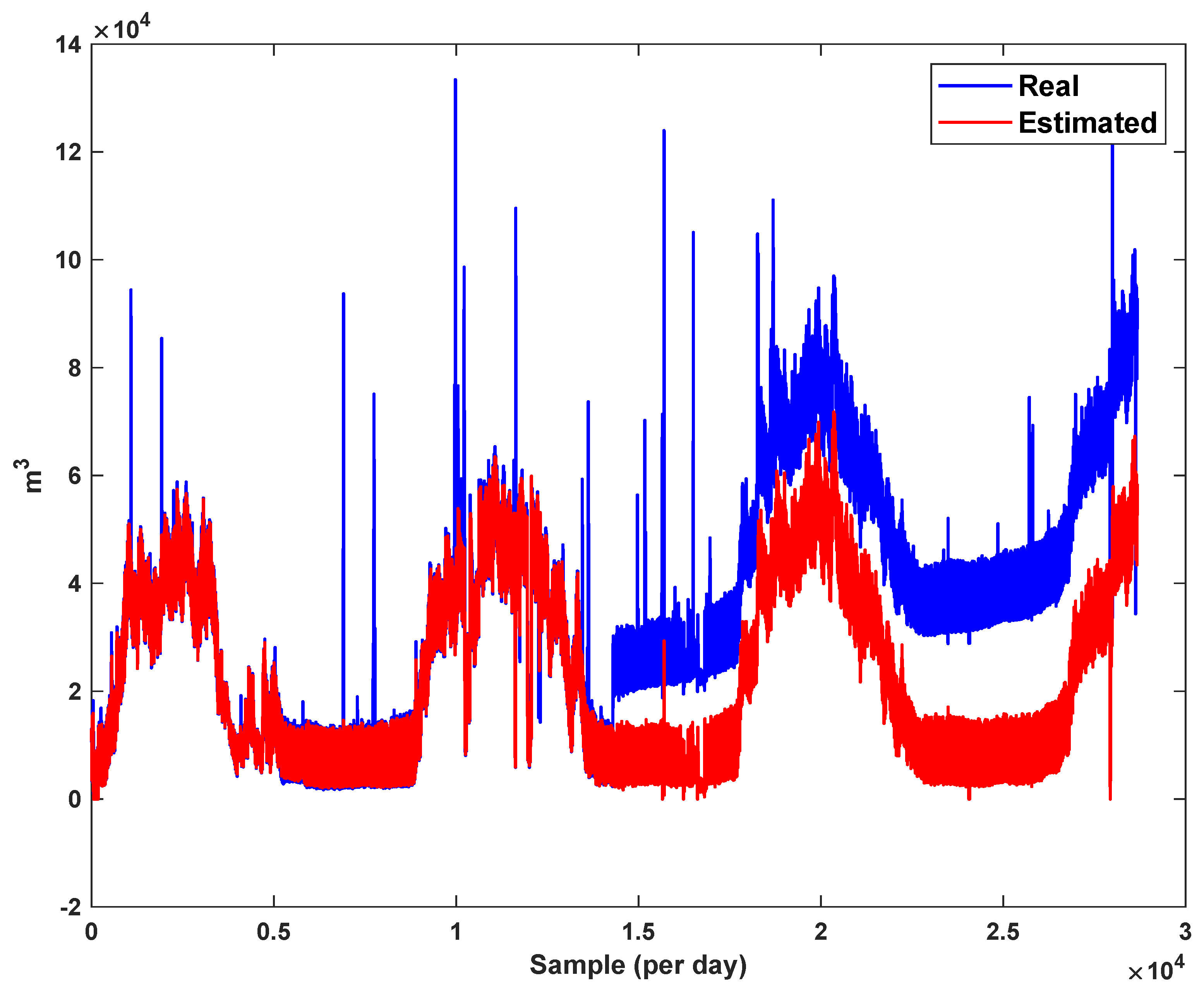
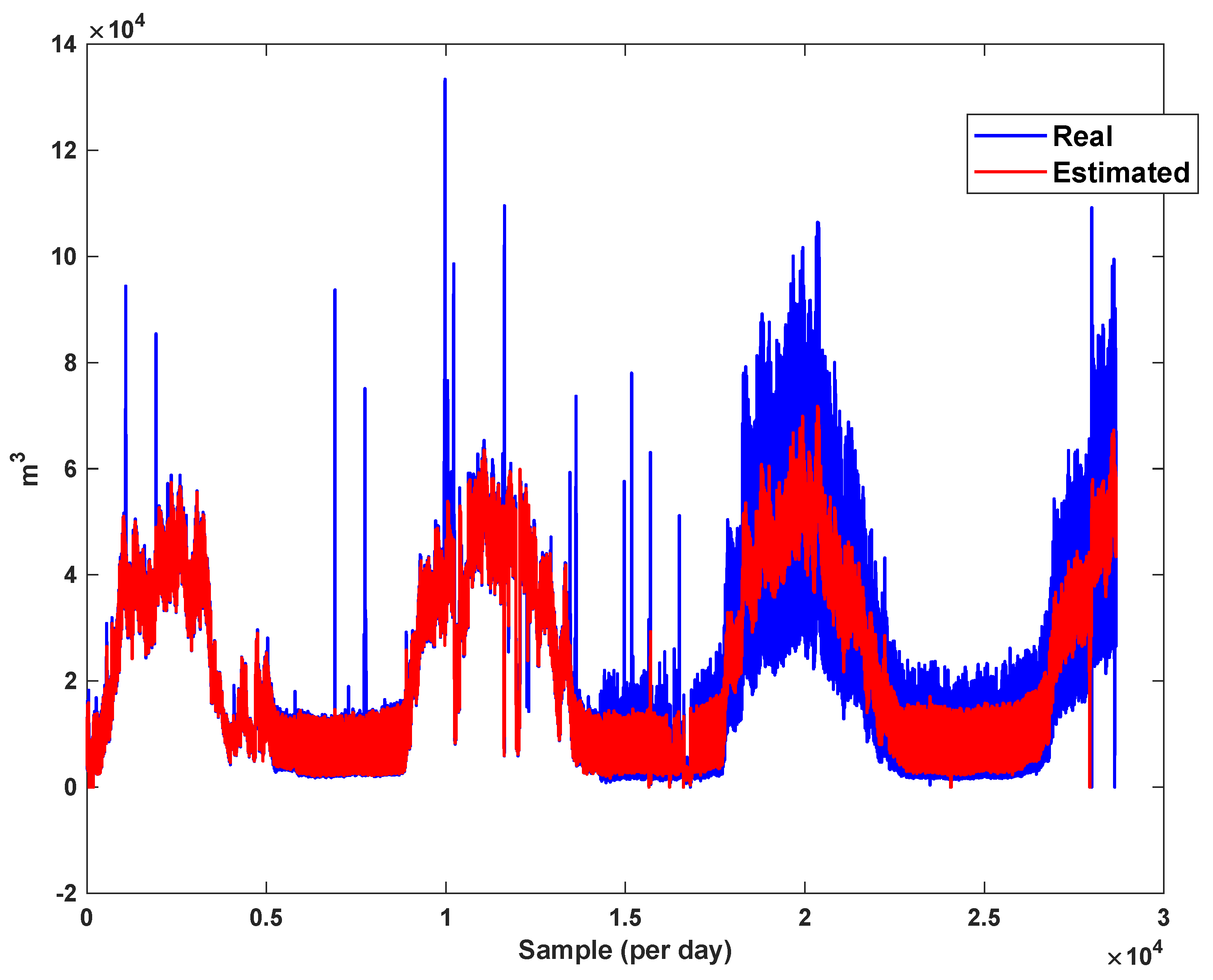
7.1. Modeling
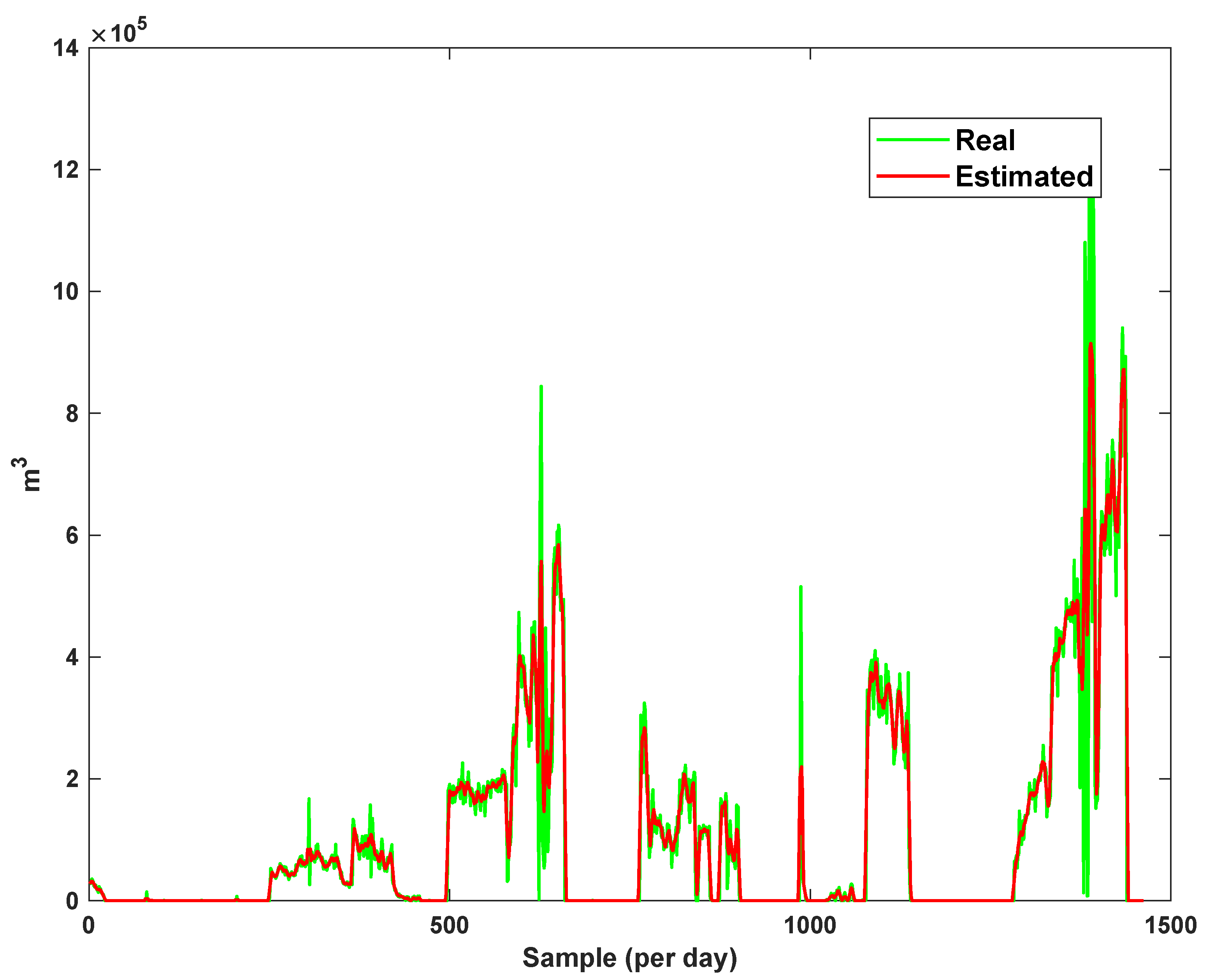
7.2. Fault Detection
8. Conclusions
Author Contributions
Funding
Institutional Review Board Statement
Informed Consent Statement
Data Availability Statement
Acknowledgments
Conflicts of Interest
References
- Tian, M.W.; Talebizadehsardari, P. Energy cost and efficiency analysis of building resilience against power outage by shared parking station for electric vehicles and demand response program. Energy 2021, 215, 119058. [Google Scholar] [CrossRef]
- Lei, Y.; Lin, J.; He, Z.; Kong, D. A method based on multi-sensor data fusion for fault detection of planetary gearboxes. Sensors 2012, 12, 2005–2017. [Google Scholar] [CrossRef] [Green Version]
- Huang, L. An improved phase difference detection method for a Coriolis flowmeter. Measurement 2021, 172, 108862. [Google Scholar] [CrossRef]
- Clavijo, N.; Melo, A.; Soares, R.M.; Campos, L.F.D.O.; Lemos, T.; Câmara, M.M.; Anzai, T.K.; Diehl, F.C.; Thompson, P.H.; Pinto, J.C. Variable Selection for Fault Detection Based on Causal Discovery Methods: Analysis of an Actual Industrial Case. Processes 2021, 9, 544. [Google Scholar] [CrossRef]
- Jiang, W.; Shen, T. Nonlinear observer-based exhaust manifold pressure estimation and fault detection for gasoline engines with exhaust gas recirculation. Int. J. Engine Res. 2021, 22, 1377–1392. [Google Scholar] [CrossRef]
- Varvani Farahani, A.; Montazeri, M. Multi-phase flow measurement in a gas refinery using decentralized Lyapunov—Based adaptive observer. Trans. Inst. Meas. Control 2021, 43, 700–716. [Google Scholar] [CrossRef]
- Medina-García, J.; Sánchez-Rodríguez, T.; Galán, J.A.G.; Delgado, A.; Gómez-Bravo, F.; Jiménez, R. A wireless sensor system for real-time monitoring and fault detection of motor arrays. Sensors 2017, 17, 469. [Google Scholar] [CrossRef] [Green Version]
- Yang, F.; Xiao, D.; Shah, S.L. Optimal sensor location design for reliable fault detection in presence of false alarms. Sensors 2009, 9, 8579–8592. [Google Scholar] [CrossRef] [Green Version]
- Mattera, C.G.; Quevedo, J.; Escobet, T.; Shaker, H.R.; Jradi, M. A method for fault detection and diagnostics in ventilation units using virtual sensors. Sensors 2018, 18, 3931. [Google Scholar] [CrossRef] [Green Version]
- Jderu, A.; Soto, M.A.; Enachescu, M.; Ziegler, D. Liquid flow meter by fiber-optic sensing of heat propagation. Sensors 2021, 21, 355. [Google Scholar] [CrossRef]
- Zhang, F.; Wang, Y.; Gao, Y. A Novel Method of Fault Detection and Identification in a Tightly Coupled, INS/GNSS-Integrated System. Sensors 2021, 21, 2922. [Google Scholar] [CrossRef]
- Zhao, H.; Luo, H.; Wu, Y. A Data-Driven Scheme for Fault Detection of Discrete-Time Switched Systems. Sensors 2021, 21, 4138. [Google Scholar] [CrossRef]
- Gamero, M.; Kim, W.S.; Hong, S.; Vorobiev, D.; Morgan, C.D.; Park, S.I. Multimodal Sensing Capabilities for the Detection of Shunt Failure. Sensors 2021, 21, 1747. [Google Scholar] [CrossRef]
- Buffa, S.; Fouladfar, M.H.; Franchini, G.; Lozano Gabarre, I.; Andrés Chicote, M. Advanced Control and Fault Detection Strategies for District Heating and Cooling Systems—A Review. Appl. Sci. 2021, 11, 455. [Google Scholar] [CrossRef]
- Cecconi, F.; Rosso, D. Soft Sensing for On-Line Fault Detection of Ammonium Sensors in Water Resource Recovery Facilities. Environ. Sci. Technol. 2021, 55, 10067–10076. [Google Scholar] [CrossRef]
- Zhang, X.; Luo, H.; Li, K.; Kaynak, O. Time-Domain Frequency Estimation with Application to Fault Diagnosis of the UAVs Blade Damage. IEEE Trans. Ind. Electron. 2021. [Google Scholar] [CrossRef]
- Tian, M.; Yan, S.; Tian, X. Discrete approximate iterative method for fuzzy investment portfolio based on transaction cost threshold constraint. Open Phys. 2019, 17, 41–47. [Google Scholar] [CrossRef]
- Gareev, A.; Minaev, E.Y.; Stadnik, D.; Davydov, N.; Protsenko, V.; Popelniuk, I.; Nikonorov, A.; Gimadiev, A. Machine-learning algorithms for helicopter hydraulic faults detection: Model based research. J. Phys. Conf. Ser. 2019, 1368, 052027. [Google Scholar] [CrossRef]
- Gareev, A.; Stadnik, D.; Popelniuk, I.; Davydov, N.; Minaev, E.; Protsenko, V.; Gimadiev, A.; Nikonorov, A. Neural networks with simulated data for the faults detection in hydraulic systems. In Proceedings of the 2020 International Conference on Information Technology and Nanotechnology (ITNT), Samara, Russia, 26–29 May 2020; pp. 1–4. [Google Scholar]
- Ontiveros-Robles, E.; Castillo, O.; Melin, P. Towards Asymmetric Uncertainty Modeling in Designing General Type-2 Fuzzy Classifiers for Medical Diagnosis. Expert Syst. Appl. 2021, 183, 115370. [Google Scholar] [CrossRef]
- Andrade, A.; Lopes, K.; Lima, B.; Maitelli, A. Development of a methodology using artificial neural network in the detection and diagnosis of faults for pneumatic control valves. Sensors 2021, 21, 853. [Google Scholar] [CrossRef]
- Yu, H.; Wang, T. A Method for Real-Time Fault Detection of Liquid Rocket Engine Based on Adaptive Genetic Algorithm Optimizing Back Propagation Neural Network. Sensors 2021, 21, 5026. [Google Scholar] [CrossRef]
- Gareev, A.; Protsenko, V.; Stadnik, D.; Greshniakov, P.; Yuzifovich, Y.; Minaev, E.; Gimadiev, A.; Nikonorov, A. Improved Fault Diagnosis in Hydraulic Systems with Gated Convolutional Autoencoder and Partially Simulated Data. Sensors 2021, 21, 4410. [Google Scholar] [CrossRef]
- Bai, M.; Liu, J.; Ma, Y.; Zhao, X.; Long, Z.; Yu, D. Long short-term memory network-based normal pattern group for fault detection of three-shaft marine gas turbine. Energies 2021, 14, 13. [Google Scholar] [CrossRef]
- Wu, Y.; Guo, H.; Song, H.; Deng, R. Fuzzy inference system application for oil-water flow patterns identification. arXiv 2021, arXiv:2105.11181. [Google Scholar]
- Alkinani, H.H.; Al-Hameedi, A.T.T.; Dunn-Norman, S. Data-driven recurrent neural network model to predict the rate of penetration: Upstream Oil and Gas Technology. Upstream Oil Gas Technol. 2021, 7, 100047. [Google Scholar] [CrossRef]
- Ge, X.; Wang, B.; Yang, X.; Pan, Y.; Liu, B.; Liu, B. Fault detection and diagnosis for reactive distillation based on convolutional neural network. Comput. Chem. Eng. 2021, 145, 107172. [Google Scholar] [CrossRef]
- Roshani, M.; Phan, G.T.; Ali, P.J.M.; Roshani, G.H.; Hanus, R.; Duong, T.; Corniani, E.; Nazemi, E.; Kalmoun, E.M. Evaluation of flow pattern recognition and void fraction measurement in two phase flow independent of oil pipeline’s scale layer thickness. Alex. Eng. J. 2021, 60, 1955–1966. [Google Scholar] [CrossRef]
- Korkerd, K.; Soanuch, C.; Gidaspow, D.; Piumsomboon, P.; Chalermsinsuwan, B. Artificial neural network model for predicting minimum fluidization velocity and maximum pressure drop of gas fluidized bed with different particle size distributions. S. Afr. J. Chem. Eng. 2021, 37, 61–73. [Google Scholar]
- Liu, Z.; Mohammadzadeh, A.; Turabieh, H.; Mafarja, M.; Band, S.S.; Mosavi, A. A New Online Learned Interval Type-3 Fuzzy Control System for Solar Energy Management Systems. IEEE Access 2021, 9, 10498–10508. [Google Scholar] [CrossRef]
- Vafaie, R.H.; Mohammadzadeh, A.; Piran, M. A new type-3 fuzzy predictive controller for MEMS gyroscopes. Nonlinear Dyn. 2021, 106, 381–403. [Google Scholar] [CrossRef]
- Cao, Y.; Raise, A.; Mohammadzadeh, A.; Rathinasamy, S.; Band, S.S.; Mosavi, A. Deep learned recurrent type-3 fuzzy system: Application for renewable energy modeling/prediction. Energy Rep. 2021, in press. [Google Scholar]
- Gheisarnejad, M.; Mohammadzadeh, A.; Farsizadeh, H.; Khooban, M.H. Stabilization of 5G telecom Converter-Based Deep Type-3 Fuzzy Machine Learning Control for Telecom Applications. IEEE Trans. Circuits Syst. II:= Express Briefs 2021. [Google Scholar] [CrossRef]
- Mohammadzadeh, A.; Sabzalian, M.H.; Zhang, W. An interval type-3 fuzzy system and a new online fractional-order learning algorithm: Theory and practice. IEEE Trans. Fuzzy Syst. 2019, 28, 1940–1950. [Google Scholar] [CrossRef]
- Qasem, S.N.; Ahmadian, A.; Mohammadzadeh, A.; Rathinasamy, S.; Pahlevanzadeh, B. A type-3 logic fuzzy system: Optimized by a correntropy based Kalman filter with adaptive fuzzy kernel size. Inf. Sci. 2021, 572, 424–443. [Google Scholar] [CrossRef]
- Moustapha, A.I.; Selmic, R.R. Wireless sensor network modeling using modified recurrent neural networks: Application to fault detection. IEEE Trans. Instrum. Meas. 2008, 57, 981–988. [Google Scholar] [CrossRef]
- Khanjani, M.; Ezoji, M. Electrical fault detection in three-phase induction motor using deep network-based features of thermograms. Measurement 2021, 173, 108622. [Google Scholar] [CrossRef]
- Kumbhar, S.G.; Sudhagar, E. An integrated approach of Adaptive Neuro-Fuzzy Inference System and dimension theory for diagnosis of rolling element bearing. Measurement 2020, 166, 108266. [Google Scholar] [CrossRef]


| Method | ||||
|---|---|---|---|---|
| Error Type | NT3FLS | RFNN [36] | SVM-NN [37] | NFLS [38] |
| Bias | 97 | 90 | 84 | 91 |
| Scaling | 98 | 88 | 85 | 92 |
| High noise | 89 | 81 | 80 | 85 |
| Hard error | 88 | 77 | 81 | 80 |
| Noise Variance | FLS | |||
|---|---|---|---|---|
| Type-1 | Type-2 | Singleton Type-3 | Non-Singleton Type-3 | |
| - | 0.2208 | 0.1365 | 0.0124 | 0.0117 |
| 0.01 | 0.3481 | 0.2470 | 0.1029 | 0.0921 |
| 0.1 | 0.8427 | 0.4578 | 0.3547 | 0.1804 |
Publisher’s Note: MDPI stays neutral with regard to jurisdictional claims in published maps and institutional affiliations. |
© 2021 by the authors. Licensee MDPI, Basel, Switzerland. This article is an open access article distributed under the terms and conditions of the Creative Commons Attribution (CC BY) license (https://creativecommons.org/licenses/by/4.0/).
Share and Cite
Wang, J.-h.; Tavoosi, J.; Mohammadzadeh, A.; Mobayen, S.; Asad, J.H.; Assawinchaichote, W.; Vu, M.T.; Skruch, P. Non-Singleton Type-3 Fuzzy Approach for Flowmeter Fault Detection: Experimental Study in a Gas Industry. Sensors 2021, 21, 7419. https://0-doi-org.brum.beds.ac.uk/10.3390/s21217419
Wang J-h, Tavoosi J, Mohammadzadeh A, Mobayen S, Asad JH, Assawinchaichote W, Vu MT, Skruch P. Non-Singleton Type-3 Fuzzy Approach for Flowmeter Fault Detection: Experimental Study in a Gas Industry. Sensors. 2021; 21(21):7419. https://0-doi-org.brum.beds.ac.uk/10.3390/s21217419
Chicago/Turabian StyleWang, Jing-he, Jafar Tavoosi, Ardashir Mohammadzadeh, Saleh Mobayen, Jihad H. Asad, Wudhichai Assawinchaichote, Mai The Vu, and Paweł Skruch. 2021. "Non-Singleton Type-3 Fuzzy Approach for Flowmeter Fault Detection: Experimental Study in a Gas Industry" Sensors 21, no. 21: 7419. https://0-doi-org.brum.beds.ac.uk/10.3390/s21217419