
A Method for Identification and Assessment of Radioxenon Plumes by Absorption in Polycarbonates


Faculty of Physics, University of Sofia “St. Kliment Ohridski”, 5 James Bourchier Blvd., 1164 Sofia, Bulgaria
*
Author to whom correspondence should be addressed.
Sensors 2021, 21(23), 8107; https://0-doi-org.brum.beds.ac.uk/10.3390/s21238107
Submission received: 27 September 2021
/
Revised: 29 November 2021
/
Accepted: 30 November 2021
/
Published: 3 December 2021
(This article belongs to the Special Issue Detection and Measurement of Radioactive Noble Gases)
Abstract
:A method for the retrospective evaluation of the integrated activity concentration of 133Xe during radioxenon plumes and the moment of the plume’s center is proposed and explored by computer modeling. The concept is to use a specimen of polycarbonate material (a stack of Makrofol N foils of thickness 120 µm and 40 µm in 1 L non-hermetic Marinelly beaker) that is placed in the environment or in a controlled nuclear or radiopharmaceutical facility. On a regular basis or incidentally, the specimen may be retrieved and gamma spectrometry in two consecutive time intervals with durations of 8 h and 16 h is performed. To assess the performance of the method, 133Xe plumes of various integrated activity concentrations and with a duration of up to 10 h are simulated and analyzed, assuming that the measurement starts with a delay of up to one day after the moment of the plume center. It is found that the deviation between the estimates by the method and their true values are within a few percent. Depending on the delay, events of integrated 133Xe activity concentration 250–1000 Bq h m−3 might be qualitatively identified. At levels >10,000 Bq h m−3, the uncertainty of the quantitative estimates might be ≤10%.
1. Introduction
Among the man-made radioactive noble gases, the isotopes of xenon (radioxenon, isotopes of interest are 135Xe, 133Xe, 133mXe and 131mXe) attract particular attention. These isotopes are released from nuclear and radiopharmaceutical facilities and from hospitals, where 133Xe is administered to patients. They are among the key radionuclides whose release from nuclear power plants (NPPs) has to be monitored [1]. In the event of a nuclear emergency, most of their inventory in the nuclear installation may be released into the environment [2]. Radioxenon plays a key role in the control of the Treaty on the Non-Proliferation of Nuclear Weapons and the Comprehensive Test Ban Treaty (CTBT) and a world monitoring network has been set up for this purpose [3]. In the environment, the concentrations of 133Xe usually exceed those of other xenon isotopes by several orders of magnitude [4], but, after a subsurface nuclear explosion, the ratio of 135Xe/133Xe may be four orders of magnitude larger compared, for instance, to a reactor release [5]. The estimated release of 133Xe from NPPs in North America and Europe ranges within 107–1011 Bq/day per one NPP unit [6], mostly as continuous emissions. The emissions from radiopharmaceutical factories are substantially higher [7] and, usually, these are “pulse” short-term releases, reaching activity of 1015 Bq in several hours, in some cases [4]. The 133Xe release after the Chernobil accident was estimated to be between 1.33 × 10¹⁷ and 6.5 × 10¹⁸ Bq [8] and the 133Xe release after the Fukushima Daiichi accident in 2011 was estimated to be of the order of 1019 Bq [9]. For comparison, after a 1 kt nuclear explosion of plutonium A-bomb, approximately 1015 Bq of 133Xe will be emitted within three hours of the explosion [10,11].
Continuous reactor releases are hardly detectable at long distances from NPPs. In contrast, radioxenon plumes with a duration of several hours and integrated over the duration of the plume 133Xe activity concentration of more than 1 kBq h m−3 may be observed tens of kilometers away from the radiopharmaceutical facilities after short-term releases of 133Xe of the order of 1013–1014 Bq [4]. At such distances, the plumes after a major nuclear emergency can be expected to have an integrated activity concentration that is 3–5 orders of magnitude greater. They are also detected at much longer distances: after the Fukushima Daiichi accident, 133Xe activity concentrations of up to 30–70 Bq m−3 were detected at distances >6500 km from the site of emergency [12,13]. The plumes at longer distances also last longer due to the plume dispersion during atmospheric transport.
Measuring 133Xe in the environment is a challenge. Thus far, there are no compact and mobile monitors that are sufficiently sensitive to be used for measurement in the environment around nuclear and radiopharmaceutical facilities. The sensitivity of the stationary monitors used in nuclear installation is not sufficient for environmental control, and, in the case of a major nuclear emergency, they may become inoperative. The radioxenon detection systems used in CTBT stations are highly sensitive, but, after a major nuclear emergency, they may reach their upper limit of detection and become inoperative. On the other hand, strategic decisions rely on information about 133Xe in the environment, especially after a nuclear emergency, accidental release from nuclear and radiopharmaceutical facilities or in the case of possible clandestine nuclear actions.
The use of the high absorption ability of noble gases by bisphenol-A based polycarbonates (BPA-PCs) [14] for 222Rn measurements was first proposed in 1999 [15] and for the measurements of 85Kr and 133Xe in 2004 [16]. Since then, many studies have focused on the further development of this “polycarbonate method” for natural [17] and man-made radioactive noble gases [18,19,20,21]. In particular, different BPA-PCs have been studied and Makrofol N® (Bayer AG) has been identified as the material that has the highest absorption ability for noble gases [22,23,24]. Thus far, the potential of this method for 133Xe measurement has been studied for long-term (days/weeks) continuous exposures [19,21]. However, accidental radioxenon releases, as well as those from radiopharmaceutical facilities, are mostly short-term “pulses”, which are registered in the close environment as radioxenon plumes with a duration of several hours [4].
In this work, we propose a method to identify, qualitatively, 133Xe plumes and to evaluate, quantitatively, the integrated 133Xe activity concentration and the moment of the plume center. The method consists of placing in the environment or within the controlled facility of polycarbonate specimens formed as a stack of Makrofol N foils of two different thicknesses, which are placed in a non-hermetic canister. The specimens can be left for a long time and taken for analysis only in the case of suspected high radioxenon release or on a regular basis, e.g., daily, for performing regular control. Then, the specimens are transported to a laboratory, which may be distant from the point of exposure, and measured via HPGe gamma spectrometry, using the 81 keV line of 133Xe. By measuring the signal (net area of the 81 keV peak spectral region of interest) in two different time intervals, the integrated activity concentration of 133Xe during the plume and the time (before the start of the measurement) of the “center of the plume” can be evaluated. By computer modeling of realistic situations, it is demonstrated that the method provides feasible results and is sufficiently sensitive in the range that is frequently encountered in the environment, e.g., around radiopharmaceutical factories [4]. The specimen can be analyzed up to one day after the plume has dissipated.
2. Materials and Methods
2.1. The Concept and Basics of the Method
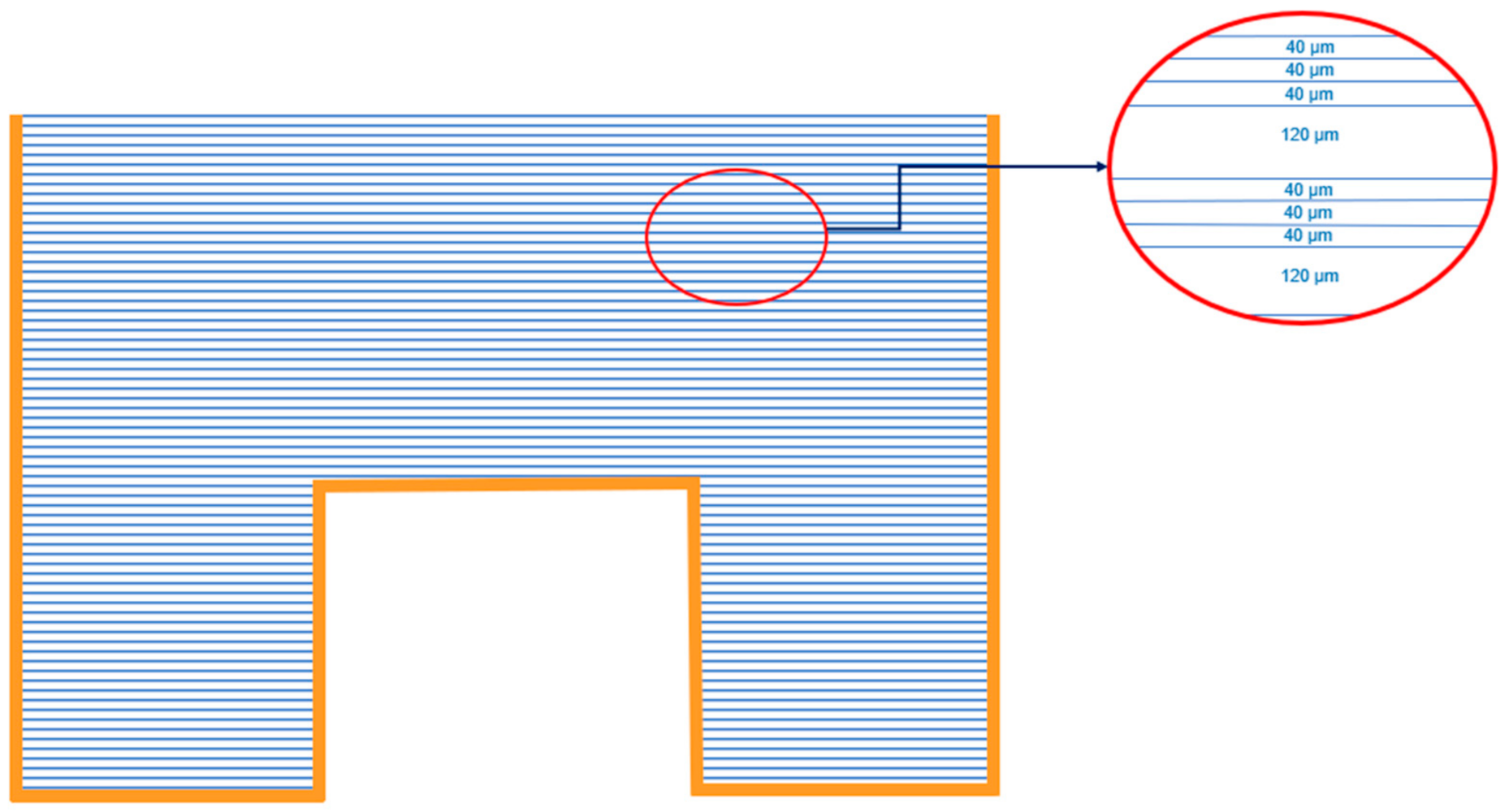
Here, we employ the concept of a “composite absorber”, consisting of a stack of absorbing foils. When the foils are not hermetically stuck together, the noble gas may penetrate freely between them. Initially, this concept was proposed and tested for radon measurement [22,26,27,28,29] and further evaluated for 133Xe, too [19]. Previous experiments with 222Rn have shown good agreement between the theoretical modeling of such “composite absorbers” and experimental results [29]. For simulation purposes, the following experimental setup is assumed, namely Makrofol N foils of thickness 40 μm and 120 μm, stuck together and placed in a canister, specifically a 1 L Marinelli beaker, as shown in Figure 2. Half of the volume of the beaker is filled with 40 μm and half of it with 120 μm, and the foils of each type can be considered evenly distributed within the volume.
The transport of a radioactive isotope of a noble gas in a polycarbonate is described by the diffusion equation with radioactive decay [18,21,30]. For the geometry of thin foils of thickness L, it is given by Equation (1) [30]:
where n is the atomic concentration of the noble gas in the polycarbonate material, x = 0 and x = L are the coordinates of the foil boundaries, D is the diffusion coefficient of xenon in the polycarbonate material, and λ is the decay constant of the isotope (in the present case, this is 133Xe). During exposure, the initial and boundary conditions are n(x, t = 0) = 0 and n(x = 0, t) = n(x = L, t) = Kn0(t), where n0 is the atom concentration of the noble gas in the ambient air and K is the “partition coefficient” (dimensionless solubility) of the gas in the material (K = ratio of the concentration in an “infinitely” thin surface layer of the material to that in the air). After exposure, the boundary conditions are zero and the initial distribution of n within the foil is that at the end of the preceding exposure. This model was found to perfectly fit the experimental data [18,21,24,30].
The exact solutions of Equation (1) have been obtained elsewhere [18,30]. According to these solutions, during exposure to a constant activity concentration cA in air (cA = λn0), the growth in activity in a stack of foils of thickness L and of total volume V can be expressed as:
where LD is the diffusion length of the considered isotope in the material () and the constants λ2k+1 are determined as follows:
Here, values of K = 17.2 and LD (133Xe) = 87.8 μm were used, according to data in Ref. [24]. In Ref. [24], LD was reported for 131mXe, and, as the diffusion coefficient for all Xe isotopes is the same, it was recalculated for 133Xe as follows:
After the end of exposure at moment T, the activity decreases due to the radioactive decay and outgazing. The process is described by expression (5) [30]:
where t is the time after the end of exposure. Notably, the thinner the foil, the faster is the decrease in the activity [19].
Let A1(t) be the activity, according to Equation (5), of a volume V filled with foils of L = L1 (in the present case, L1 = 40 µm) and A2(t) is when it is filled with foils of L = L2 (L2 = 120 µm). Then, the activity of the composite absorber of volume V, when V is filled with foils of thickness L1 and another V with foils of L2, is given by Equation (6):
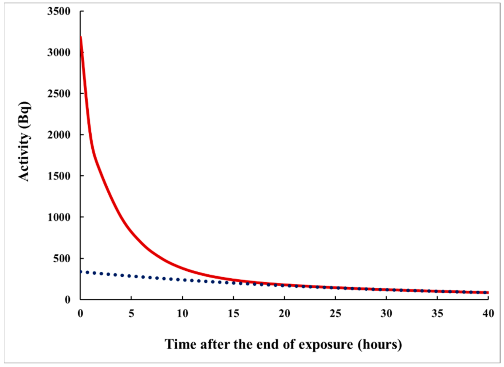
where the constants correspond to foils of thickness Li (i = 1,2). Figure 3 illustrates the time dependence of A(t).
When using HPGe gamma spectrometry, the measured signal (S) is the net-area of the 81 keV peak region of interest (ROI). In data processing, the detection efficiency (ε) and the probability (p) for 81 keV gamma emission in the 133Xe decay should be taken into account. For modeling purposes, it is assumed that the specimens taken for analysis are measured by HPGe gamma spectrometry in two consecutive time intervals: the first of duration t1 = 8 h (signal S1) and the second of duration t2 = 16 h (S2)—the duration of the whole measurement is t1 + t2 = 24 h. In the general case, the time interval when the plume has occurred is not known and some time for transportation of the specimen to the measuring laboratory may be needed. Therefore, the measurement starts with some delay τd after the end of the plume (or τ after its “center”, for rectangular plumes of duration T: τ = τd + T/2). Therefore, the modeled signals S1 and S2 in the first and the second interval are as follows:
where the activity A(t) is that given by Equation (6). Respectively, for S2, one obtains:
It could be seen in Figure 3 that, after sufficient delay (e.g., >20 h) following the end of exposure, the time dependence is determined mainly by one component of the sum (7): that with , which is the smallest constant in the set of constants (in present case, = 0.0346 h−1). This component is also dominating in the times when S2 is acquired (t > 8 h). Therefore, at the times when this component dominates, the following approximation becomes useful:
The next approximation is for a plume duration of a few hours. With the quoted λ1(2), for such plumes, λ1(2)T is much smaller than one, and 1-exp() ≈ , which, for T = 1 h, is valid within 2%; for T = 8 h, within 8%, and for T = 10 h, within 15%. Therefore,
Using the approximations (7) and (8), one obtains, if the conditions of the approximations are met,
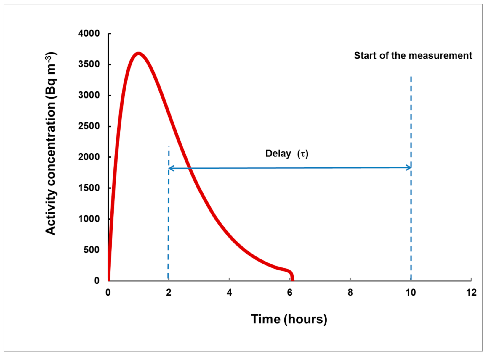
where IA = cA0T is the time-integrated concentration of 133Xe for the considered rectangular plume. In addition, for plumes of different shapes, the end of the plume is not a well-defined moment and, preferably, the delay (τ) should be measured from its center, as shown in Figure 4. The following “working hypothesis”, raised for plumes of any shape and of any duration, so far not exceeding 10 h, is at the core of the method:
- For measurement in two consecutive time intervals, (0–8 h) and (8–24 h), the observed ratio S1/S2 can be correlated with the delay τ, measured from the center of the plume, and the dependence τ = τ(S1/S2) can be used to assess the delay τ of a plume of any shape.
- The signal S2 may be expressed as:
The dependence τ(S1/S2) was obtained by simulation of rectangular plumes of different duration and different delay τ, and looking for the best fit, which can be interpolated by analytical expression. Using the same simulation data, the corrective function g(τ) was modeled by the following expression, obtained from Equation (12):
where S2(true) is that calculated by Equation (8).
When the above conditions are met and τ(S1/S2) and g(τ) are known, for any arbitrary plume, using the measured S1 and S2, the delay τ is determined from τ = τ(S1/S2) and IA is determined as follows:
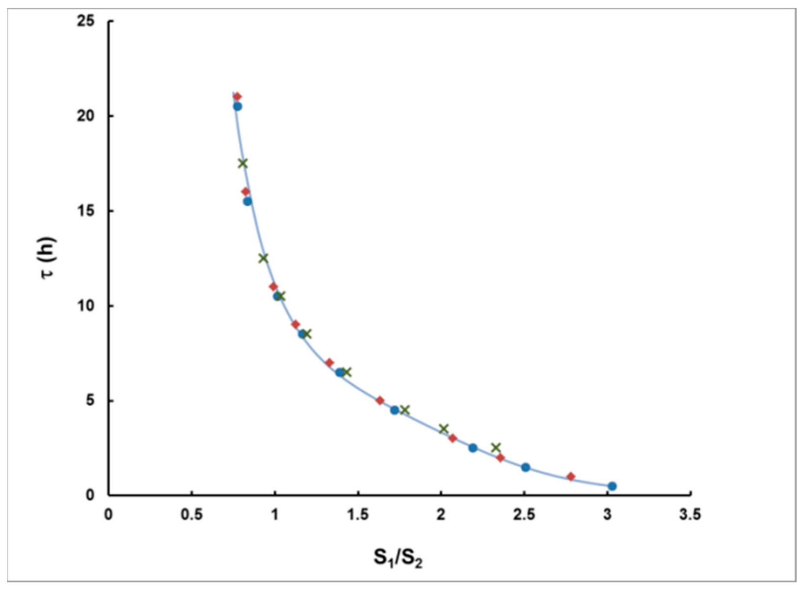
Computer modeling, based on the analytical expressions described in this paper, was carried out in order to prove that, based on this hypothesis, one may obtain reliable results for the delay τ and the integrated activity concentration IA. For different cA, T and τ, the signals S1 and S2 were calculated using the exact expressions (7) and (8). The correlation between τ and S1/S2 is illustrated in Figure 5. The dependence is practically one and the same for rectangular plumes of duration 1–5 h.
The data are very well-interpolated by the following expression (the curve in Figure 5), which is hereafter used to determine τ from S1/S2:
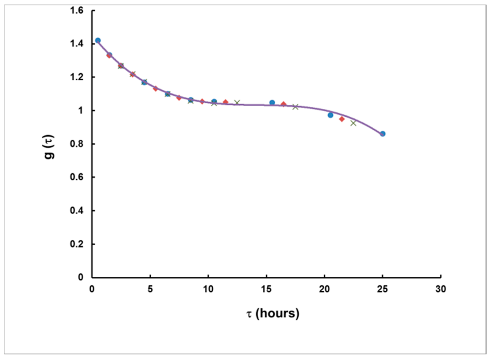
The results for g are illustrated in Figure 6. As seen, the results depend on τ, but practically not on T.
This dependence was very well-interpolated analytically, by the following polynomial:
where τ is previously obtained by Equation (15). The obtained interpolations of τ(S1/S2) and g(τ) were used in the data processing of simulated plumes of any shape and of different delay.
2.2. Estimating the Uncertainty and the Level of Plume Identification
Both IA and τ are functions of S1 and S2, which are uncorrelated variables. In real measurements, they are random numbers of “counting uncertainty” σ(S1) and σ(S2), which can be determined by the Poisson distribution of the total number of counts and the background. Using the interpolation expressions for τ(S1/S2), g(τ(S1/S2)) and replacing them in Equation (14), one obtains the function IA (S1, S2). Then, the uncertainties are calculated, using the common uncertainty propagation formulas for functions of uncorrelated variables [31]:
The level of plume identification IA(min) is the minimum level at which the signal will exceed the background at 95% probability. This problem has been considered elsewhere [32], where it has been shown that, for a “well-defined background” (assumed in our modeling), this is valid when the signal is:
3. Results
3.1. Methodological Bias in the Estimates of the of Delay and the Integrated Concentration
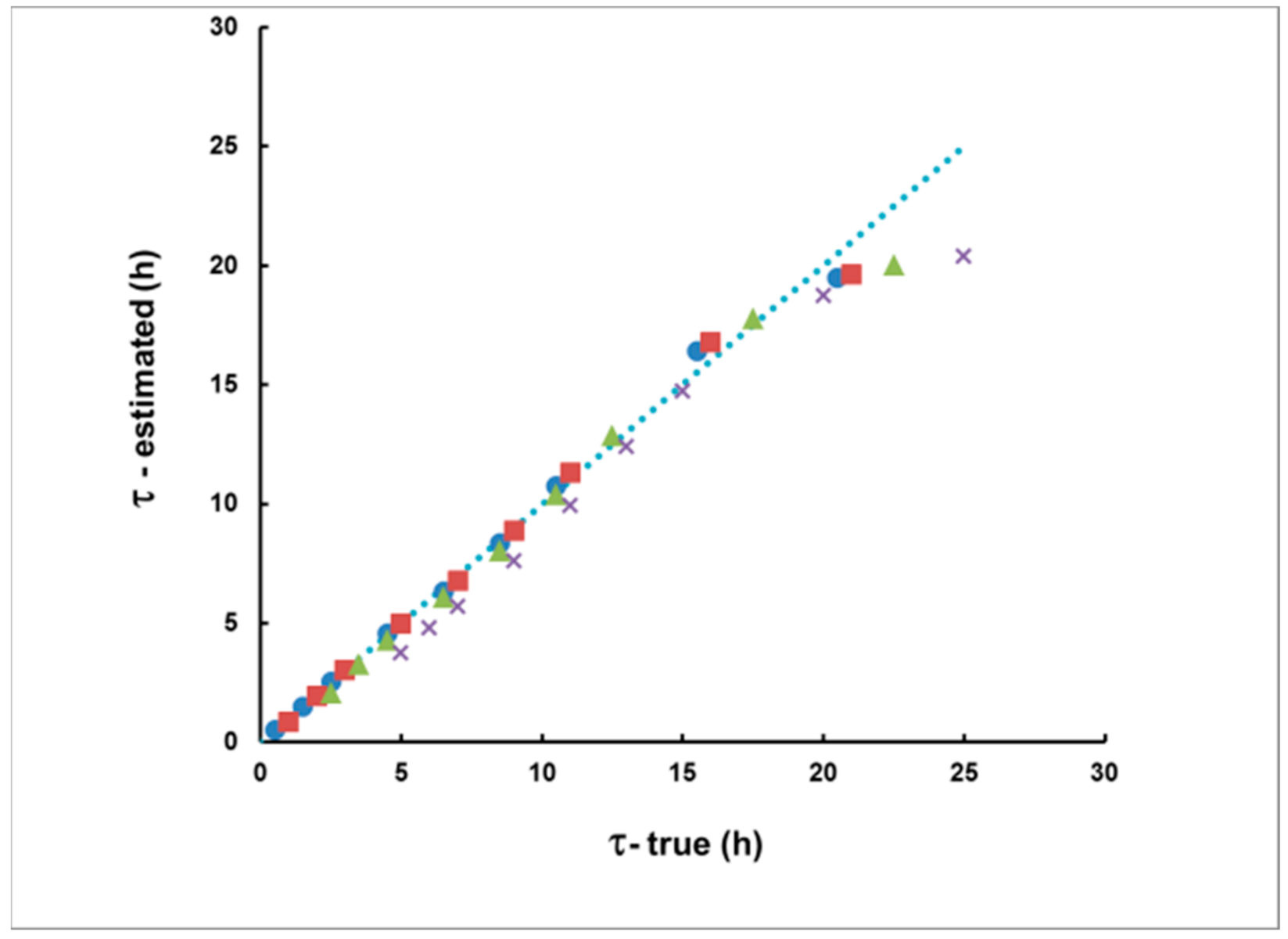
Figure 7 illustrates the agreement between the true and calculated time delay according to Equation (15). In this case, rectangular plumes with a duration of up to 10 h were considered. For time delays of up to 20 h, a very good match was observed between the true and calculated time delay values. There was a systematic bias for time delays higher than 20 h, which increased with the increase in the delay. Therefore, at this stage, the use of the proposed method should be restricted only to situations in which the measurement starts no later than 20 h after the moment of the “plume center”.
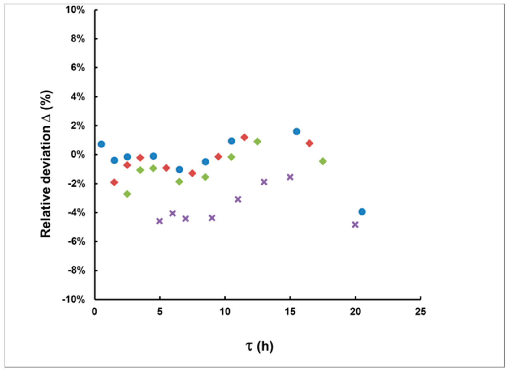
Using Equation (14) and the estimated value of the delay time, one can calculate the values of IA. Figure 8 illustrates the relative deviation of IA determined by Equation (16) from its true value for the case of rectangular plumes with a duration of up to 10 h and measurement started with a delay of up to 20 h. As seen in the figure, all relative deviations fall within 6%, while most of them fall within 2%. In most real cases, such bias will be sufficiently smaller than the uncertainty incurred by counting statistics.
3.2. Simulation of Levels of Identification and Instrumental Uncertainty
The characteristics of the gamma spectrometer employed for research and education, in our laboratory, were used in the modeling. The spectrometer was supplied with a HPGe detector (ORTEC®) of 24.9% relative efficiency and a resolution (FWHM) of 1.9 keV for the 1332 keV line of 60Co. Gamma spectrometry analysis uses the line of 133Xe with energy 81 keV (p = 0.37, see Figure 1) [25]. When the background (with a shielded detector) is measured for long time, the average counting rate in the region of interest of the 81 keV peak is approximately 1 cpm (60 imp/hour) and this value has been used in the modeling. Thus, the background counts in the first interval with a duration of 8 h will be 480 (8 × 60) and in the second interval with a duration of 16 h will be 960 (16 × 60) correspondingly.
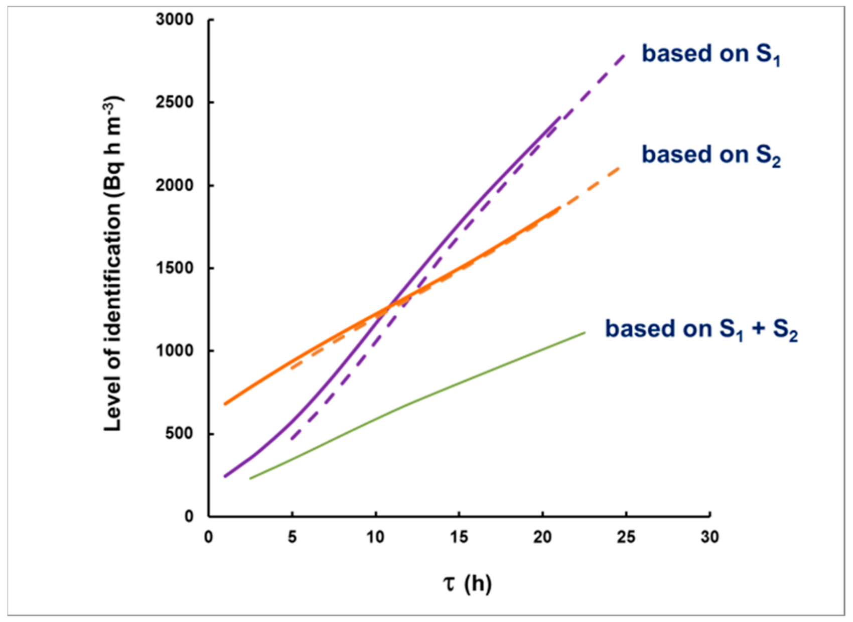
By substituting this background, one may calculate the “critical levels” Lc1, Lc2, for the corresponding intervals (see Equation (19)). The values of IA that “generate” signals S1 = LC1 or S2 = Lc2 will be “the level for qualitative identification”. This level depends on the choice of the intervals used for identification and on the time delay. The results for the level of identification after numerical simulations are illustrated in Figure 9 as dependent on the delay. As seen in this figure, if S1 + S2 is used (24 h spectrum acquisition), a plume with an integrated activity concentration greater than 1000 Bq h m−3 will lead to a signal that would exceed the background at a 95% level of confidence, and levels as low as 250 Bq h m−3 may be qualitatively identified if the measurement starts with a delay <2 h. Even measurements within the first 8 h (S1) may be conclusive for the identification of <1000 Bq h m−3, provided that the delay does not exceed 10 h. This means that most of the radioxenon plumes observed, e.g., in Ref. [4], tens kilometers away from radiopharmaceutical facilities, would be identified.
However, at levels close to the level of identification, quantitative estimates will be of great uncertainty and only qualitative identification is possible.
Assuming a well-defined background, the uncertainty in S1 and S2 due to the Poisson counting statistics will be:
We have modeled uncertainty propagation, assuming Poisson distribution of the total number of counts in the ROI for the corresponding time interval. The results are illustrated in Figure 10.
As can be seen in Figure 10, the relative uncertainty is substantially influenced by the delay time. For a delay time of 20 h, only levels greater than 20,000 Bq h m−3 can be measured within 50% relative uncertainty, while, for a delay time of 8 h, 50% relative uncertainty could be achieved even for levels of approximately 5000 Bq h m−3. The delay time of 1 h makes it possible for levels >10,000 Bq h m−3 to be evaluated with a relative uncertainty better than 10%.
3.3. Simulation of Plumes for an Arbitrary Shape
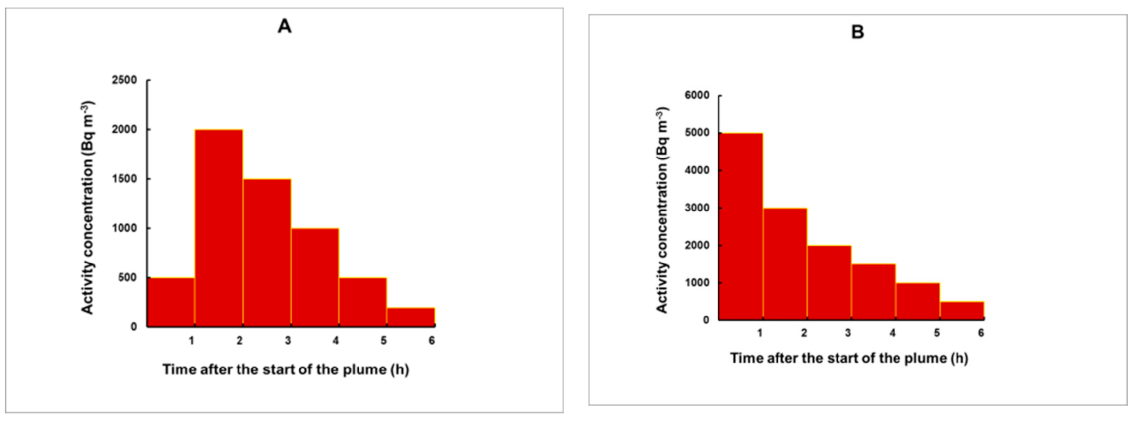
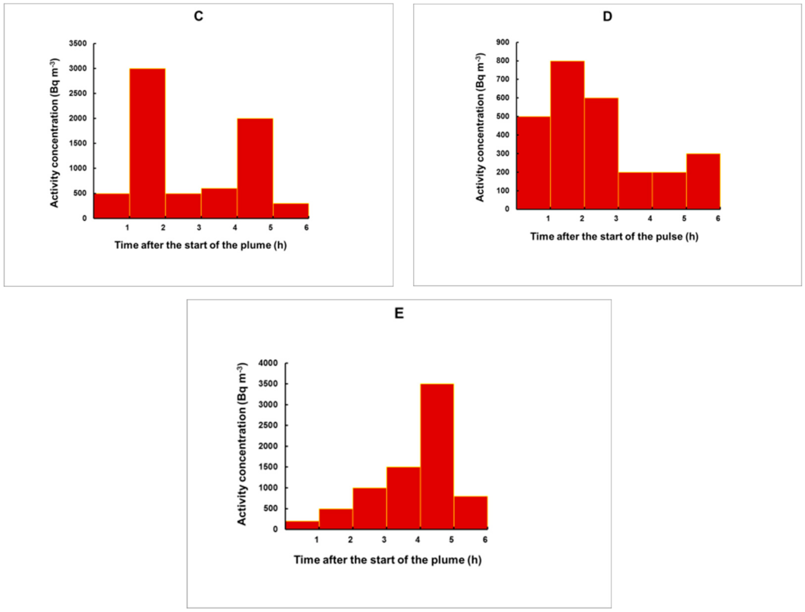
To check whether the method may work reliably for pulses with irregular shape, we simulated different plume profiles, illustrated in Figure 11.
With each plume, two “measurement delay scenarios” were considered: the first one commencing 2 h after the end of the plume and a second one commencing 8 h after the end of the plume. Because the plumes were of different shape, the delays from the plume’s center were different. The delay was calculated by Equation (15) and the integrated activity by Equation (14). The results are illustrated in Figure 12 and Figure 13.
4. Discussion and Conclusions
The present work demonstrates, by computer modeling, that, in polycarbonate specimens composed of Makrofol N foils of thickness 40 μm and 120 μm, exposed for a certain time interval in which a short-term 133Xe plume occurs, and with consecutive HPGe gamma spectrometry measurement in two time intervals, the following plume characteristics can be determined:
- The time (before the start of the gamma spectrometry measurement) at which the center of the plume was situated;
- The 133Xe activity concentration, integrated over the total duration of the plume, provided that the plume ended before the specimen was taken from the place of exposure. Otherwise, IA will refer to the time from the start of the plume until the moment when the specimen was removed for analysis.
By computer simulation of real plumes of rectangular and arbitrary shape, it was demonstrated (Figure 9) that even plumes of IA < 500 Bq h m−3 may be identified at 95% statistical significance if the measurement starts within the first 8 h after the moment of the plume center. Notably, this estimate was achieved for a gamma spectrometer of average class. The current state-of-the-art in the field of gamma spectrometry includes detectors of much better efficiency and detection systems with better suppressed background than these for the instrument whose characteristics were used. Therefore, one may anticipate that this method has the potential for better sensitivity than that estimated in the current study. Moreover, the choice of foil thickness and counting intervals in the present work was arbitrary, aiming to evaluate the feasibility of the method. Further research may model different foils and counting intervals, aiming for the optimization of the method.
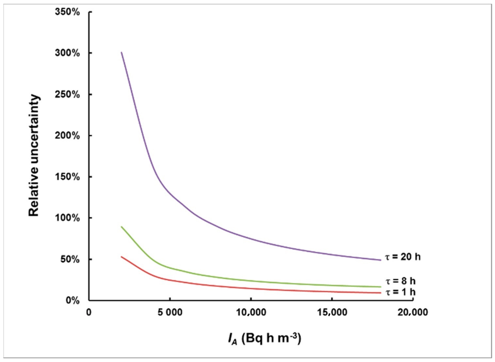
The method provides data that can be useful for the evaluation of other characteristics of the release, e.g., the total released activity. For instance, if the specimen is placed in the ventilation stack through which the activity is released, to obtain the total released activity, one simply has to multiply the determined integrated activity concentration by the air flow rate through the stack. If the specimen is exposed to the environment, the use of an atmospheric transport model along with the data from the measurement will be needed. Thus far, estimates of the released activity, especially after accidents, are associated with great uncertainties and, sometimes, only the order of magnitude of the release may be assessed. In contrast, the modeling revealed that this method may provide IA estimates of uncertainty that may be potentially less than 10% (see Figure 10). Therefore, the proposed method has the potential to facilitate a step forward in this direction.
The absorption ability of polycarbonates is not affected by most of environmental factors (pressure, fume, dust, humidity within 0–100% and even wetting of the material [33,34]). The temperature is the only environmental factor of influence, which, however, may be taken into account, provided that the temperature dependences of K and D for xenon in Makrofol N are well-known. Currently, there are data available only for room temperature (22 °C) and the current modeling is based on these data. Dedicated research to complement the data set with values for other temperatures is planned for the future.
One important challenge is to test the method experimentally. Experimental tests with 133Xe are hampered by the difficult and expensive access to certified 133Xe sources and the difficulty of creating a reference 133Xe concentration that can be precisely controlled. We plan in the future to perform such experiments using, as a surrogate of 133Xe, the isotope 222Rn, for which such tests will be much easier. Of course, this will need revision of the method to incorporate data related to 222Rn for the parameters used.
The polycarbonate material is cheap and offers a cost-efficient option to place many specimens for a long time at different locations in the environment, as well as within a controlled facility, and to use them on occasion, or periodically for regular control. Such a network of specimens may be useful after real or suspected radioxenon release from a nuclear or radiopharmaceutical facility, or to check for possible clandestine nuclear activity. The measured specimens may provide data that will complement the data from stationary monitors and may be used to refine the atmospheric transport models of the plumes. In addition, after outgazing for 10 days or more, the specimen will be suitable for use again. The analysis of the specimens may be conducted in laboratories that are far from the site of exposure, which may be very useful in the event of a nuclear emergency, where the efforts to clarify the situation become international.
Author Contributions
Conceptualization, D.P.; methodology, D.P.; software, P.S., D.P.; validation, D.P., P.S.; formal analysis, D.P.; investigation, D.P.; data curation, D.P.; writing—original draft preparation, D.P.; writing—review and editing, D.P., P.S. All authors have read and agreed to the published version of the manuscript.
Funding
This research received no external funding.
Institutional Review Board Statement
Not applicable.
Informed Consent Statement
Not applicable.
Data Availability Statement
The study did not report any data.
Acknowledgments
The authors are grateful to Tatiana Boshkova for the consultancy in HPGe gamma spectrometry, to Violina Georgieva-Duparinova for the help in preparing the illustrations and to Nadejda Gavritova-Stavreva for the help with the English editing.
Conflicts of Interest
The authors declare no conflict of interest.
References
- Commission of the European Communities. Commission recommendation of 18 December 2003 on standardised information on radioactive airborne and liquid discharges into the environment from nuclear power reactors and reprocessing plants in normal operation (notified under document No: C(2003) 4832). Off. J. Eur. Union 2004, L2, 36–46. [Google Scholar]
- Stohl, A.; Seibert, P.; Wotawa, G.; Arnold, D.; Burkhart, J.F.; Eckhardt, S.; Tapia, C.; Vargas, A.; Yasunari, T.J. Xenon-133 and caesium-137 releases into the atmosphere from the Fukushima Dai-ichi nuclear power plant: Determination of the source term, atmospheric dispersion, and deposition. Atmos. Chem. Phys. 2012, 12, 2313–2343. [Google Scholar] [CrossRef] [Green Version]
- Comprehensive Nuclear-Test-Ban Treaty Organization. Available online: https://www.ctbto.org (accessed on 15 September 2021).
- Stocki, T.J.; Armand, P.; Heinrich, P.; Ungar, R.K.; D’Amours, R.; Korpach, E.P.; Bellivier, A.; Taffary, T.; Malo, A.; Bean, M.; et al. Measurement and modelling of radioxenon plumes in the Ottawa Valley. J. Environ. Radioact. 2008, 99, 1775–1788. [Google Scholar] [CrossRef] [PubMed]
- Mitev, K.; Cassette, P. Radioactive noble gas detection and measurement with plastic scintillators. In Plastic Scintillators; Hamel, M., Ed.; Springer: Basel, Switzerland, 2021; pp. 385–423. [Google Scholar]
- Kalinowski, M.B.; Tatlisu, H. Global Radioxenon Emission Inventory from Nuclear Power Plants for the Calendar Year. Pure Appl. Geophys. 2014, 178, 2695–2708. [Google Scholar] [CrossRef]
- Saey, P.R.J.; Bean, M.; Becker, A.; Coyne, J.; D’Amours, R.; De Geer, L.-E.; Hogue, R.; Stocki, T.J.; Ungar, R.K.; Wotawa, G. A long distance measurement of radioxenon in Yellowknife, Canada, in late October 2006. Geophys. Res. Lett. 2007, 34, L20802. [Google Scholar] [CrossRef]
- International Atomic Energy Agency. Chernobyl’s Legacy: Health, Environmental and Socio-Economic Impacts and Recommendations to the Governments of Belarus, the Russian Federation and Ukraine; Kinly, D., III, Ed.; IAEA: Vienna, Austria, 2005. [Google Scholar]
- Stohl, A.; Seibert, P.; Wotawa, G. The total release of xenon-133 from the Fukushima Dai-ichi nuclear power plant accident. J. Environ. Radioact. 2012, 112, 155–159. [Google Scholar] [CrossRef] [Green Version]
- Perkins, R.W.; Casey, L.A. Radioxenons: Their Role in Monitoring a Comprehensive Test Ban Treaty; Rep. DOE/RL-96-1; Pac. Northwest Natl. Lab.: Richland, WA, USA, 1996. [Google Scholar]
- Leith, W. Geologic and Engineering Constraints on the Feasibility of Clandestine Nuclear Testing by Decoupling in Large Underground Cavities; U.S. Geol. Surv. Open File Rep.: Reston, Virginia, 2001; pp. 1–28. [Google Scholar]
- Bowyer, T.W.; Biegalski, S.R.; Cooper, M.; Eslinger, P.W.; Haas, D.; Hayes, J.C.; Miley, H.S.; Strom, D.J.; Woods, V. Elevated radioxenon detected remotely following the Fukushima nuclear accident. J. Environ. Radioact. 2011, 102, 681–687. [Google Scholar] [CrossRef]
- Sinclair, L.E.; Seywerd, H.C.J.; Fortin, R.; Carson, J.M.; Saull, P.R.B.; Coyle, M.J.; Van Brabant, R.A.; Buckle, J.L.; Desjardins, S.M.; Hall, R.M. Aerial measurement of radioxenon concentration off the west coast of Vancouver Island following the Fukushima reactor accident. J. Environ. Radioact. 2011, 102, 1018–1023. [Google Scholar] [CrossRef] [Green Version]
- Möre, H.; Hubbard, L.M. 222Rn absorption in plastic holders for alpha track detectors: A source of error. Radiat. Prot. Dosim. 1997, 74, 85–91. [Google Scholar] [CrossRef]
- Pressyanov, D.; Van Deynse, A.; Buysse, J.; Poffijn, A.; Meesen, G. Polycarbonates: A new retrospective radon monitor. In Proceedings of the IRPA Regional Congress on Radiation Protection in Central Europe, Budapest, Hungary, 23–27 August 1999; pp. 716–722. [Google Scholar]
- Pressyanov, D.S.; Mitev, K.K.; Stefanov, V.H. Measurements of 85Kr and 133Xe by absorption in Makrofol. Nucl. Instrum. Methods Phys. Res. 2004, 527, 657–659. [Google Scholar] [CrossRef]
- Pressyanov, D. Modeling a 222Rn measurement technique based on absorption in polycarbonates and track-etch counting. Health Phys. 2009, 97, 604–612. [Google Scholar] [CrossRef]
- Pressyanov, D.; Mitev, K.; Georgiev, S.; Dimitrova, I. Sorption and desorption of radioactive noble gases in polycarbonates. Nucl. Instrum. Methods Phys. Res. 2009, 598, 620–627. [Google Scholar] [CrossRef]
- Georgiev, S.; Mitev, K.; Pressyanov, D.; Boshkova, T.; Dimitrova, I. Measurement of Xe-133 in Air by Absorption in Polycarbonates—Detection Limits and Potential Applications. In Proceedings of the 2011 IEEE Nuclear Science Symposium Conference Record NP1.M-85, Valencia, Spain, 23–29 October 2011. [Google Scholar]
- Mitev, K.; Zhivkova, V.; Pressyanov, D.; Georgiev, S.; Dimitrova, I.; Gerganov, G.; Boshkova, T.; Pressyanov, D. Liquid scintillation counting of polycarbonates: A sensitive technique for measurement of activity concentration of some radioactive noble gases. Appl. Radiat. Isot. 2014, 93, 87–95. [Google Scholar] [CrossRef]
- Pressyanov, D.; Mitev, K.; Dimitrova, I.; Georgiev, S. Solubility of krypton, xenon and radon in polycarbonates. Application for measurement of their radioactive isotopes. Nucl. Instrum. Methods Phys. Res. 2011, 629, 323–328. [Google Scholar] [CrossRef]
- Tommasino, L.; Tommasino, M.C.; Viola, P. Radon-film-badges by solid radiators to complement track detector-based radon monitors. Radiat. Meas. 2009, 44, 719–723. [Google Scholar] [CrossRef]
- Mitev, K.; Cassette, P.; Georgiev, S.; Dimitrova, I.; Sabot, B.; Boshkova, T.; Tartès, I.; Pressyanov, D. Determination of 222Rn absorption properties of polycarbonate foils by liquid scintillation counting. Application to 222Rn measurements. Appl. Radiat. Isot. 2016, 109, 270–275. [Google Scholar] [CrossRef]
- Mitev, K.; Cassette, P.; Tartès, I.; Georgiev, S.; Dimitrova, I.; Pressyanov, D. Diffusion lengths and partition coefficients of 131mXe and 85Kr in Makrofol N and Makrofol DE polycarbonates. Appl. Radiat. Isot. 2018, 134, 269–274. [Google Scholar] [CrossRef]
- Laboratoire National Henri Becquerel. Available online: https://lnhb.br/donnees-nucleaires/donnees-nucleaires-tableau (accessed on 16 November 2021).
- Tommasino, L. Radon film-badges versus existing passive monitors based on track etch detectors. Nukleonika 2010, 55, 549–553. [Google Scholar]
- Tommasino, L.; Tomasino, M.C.; Espinosa, G. Radon film badges based on radon-sorption in solids. A new field for solving long-lasting problems. Rev. Mex. Fis. 2010, S56, 1–4. [Google Scholar]
- Pressyanov, D. Modeling response of radon track detectors with solid absorbers as radiators. Radiat. Meas. 2011, 46, 357–361. [Google Scholar] [CrossRef]
- Pressyanov, D.; Georgiev, S.; Dimitrova, I.; Mitev, K. Experimental study of the response of radon track detectors with solid absorbers as radiators. Radiat. Meas. 2013, 50, 141–144. [Google Scholar] [CrossRef]
- Pressyanov, D.; Georgiev, S.; Dimitrova, I.; Mitev, K.; Boshkova, T. Determination of the diffusion coefficient and solubility of radon in plastics. Radiat. Prot. Dosim. 2011, 145, 123–126. [Google Scholar] [CrossRef]
- Taylor, B.N.; Kuyatt, C.E. Guidelines for Evaluating and Expressing the Uncertainty of NIST Measurement Results. In NIST Technical Note 1297; 1994. Available online: https://emtoolbox.nist.gov/Publications/NISTTechnicalNote1297s.pdf (accessed on 20 September 2021).
- Currie, L.A. Limits for Qualitative Detection and Quantitative Determination. Anal. Chem. 1968, 40, 586–593. [Google Scholar] [CrossRef]
- Pressyanov, D.; Buysse, J.; Poffijn, A.; Van Deynse, A.; Meesen, G. Integrated measurements of 222Rn by absorption in Makrofol. Nucl. Instrum. Methods Phys. Res. 2004, 516, 203–208. [Google Scholar] [CrossRef]
- Dimitrov, D.; Pressyanov, D. The CD/DVD method as a tool for the health physics service and ventilation diagnostics in underground mines. Radiat. Prot. Dosim. 2018, 181, 30–33. [Google Scholar] [CrossRef]
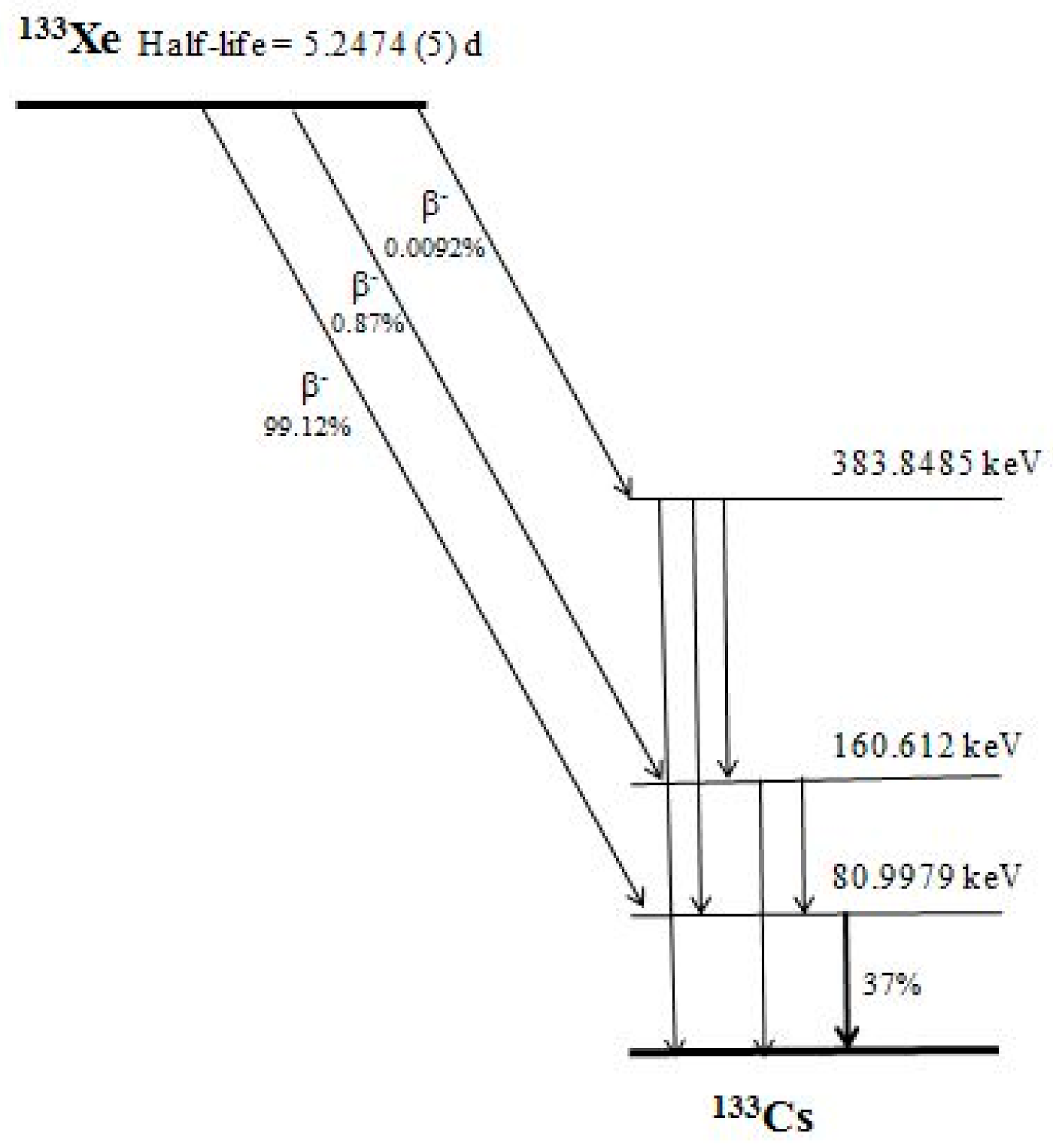
Figure 1.
Decay scheme of 133Xe. The half-life, probability of the decay modes and energy of the excited states are shown, using the data of Ref. [25]. The present method uses the gamma-line of energy 80.9972 (≈81 kev) that is of emission probability of 37%.
Figure 1.
Decay scheme of 133Xe. The half-life, probability of the decay modes and energy of the excited states are shown, using the data of Ref. [25]. The present method uses the gamma-line of energy 80.9972 (≈81 kev) that is of emission probability of 37%.

Figure 2.
Placement of Makrofol N foils in 1 L Marinelli beaker for exposure in the environment. Above one 120 μm foil, three 40 μm foils are placed and this is repeated until the volume is filled.
Figure 2.
Placement of Makrofol N foils in 1 L Marinelli beaker for exposure in the environment. Above one 120 μm foil, three 40 μm foils are placed and this is repeated until the volume is filled.

Figure 3.
The decrease in the activity in the specimen (due to radioactive decay and outgazing) after the end of exposure, according to eqn. (6). The initial activity of the specimen (at the end of exposure) is 3200 Bq. The dotted line corresponds to the “slowest component” in the sum (6), that is ~exp(). Note that the ratio A(τ)/A(t+τ) at fixed t depends on τ; therefore, τ might be correlated with S1/S2.

Figure 4.
An arbitrary example of a plume. As the “end of plume” may be not well-defined, it is preferred to use the delay from the center of the plume. The moment of this center is = (for rectangular plumes, it is T/2).
Figure 4.
An arbitrary example of a plume. As the “end of plume” may be not well-defined, it is preferred to use the delay from the center of the plume. The moment of this center is = (for rectangular plumes, it is T/2).

Figure 5.
Delay (τ) as a function of S1/S2. Simulated rectangular plumes of duration 1 h (●), 2 h (♦) and 5 h (×) are fitted by the equation (15) (the solid curve).
Figure 5.
Delay (τ) as a function of S1/S2. Simulated rectangular plumes of duration 1 h (●), 2 h (♦) and 5 h (×) are fitted by the equation (15) (the solid curve).

Figure 6.
The corrective function g as a function of τ. Points correspond to rectangular plumes of duration 1 h (●), 3 h (♦) and 5 h (×). The solid curve represents a third-degree polynomial fit to the data points (Equation (14)).
Figure 6.
The corrective function g as a function of τ. Points correspond to rectangular plumes of duration 1 h (●), 3 h (♦) and 5 h (×). The solid curve represents a third-degree polynomial fit to the data points (Equation (14)).

Figure 7.
The estimated, according to S1/S2 delay, compared with the true delay of rectangular plumes of duration 1 h (●), 2 h (■), 5 h (▲) and 10 h (×). The dotted line represents the coincidence between the estimated and true values.
Figure 7.
The estimated, according to S1/S2 delay, compared with the true delay of rectangular plumes of duration 1 h (●), 2 h (■), 5 h (▲) and 10 h (×). The dotted line represents the coincidence between the estimated and true values.

Figure 8.
The relative deviation in IA (Δ = (IA(calculated) − IA(true))/IA(true)) for delays of up to 20 h. The duration of the simulated rectangular plumes is 1 h (●), 3 h (♦), 5 h (♦) and 10 h (×).
Figure 8.
The relative deviation in IA (Δ = (IA(calculated) − IA(true))/IA(true)) for delays of up to 20 h. The duration of the simulated rectangular plumes is 1 h (●), 3 h (♦), 5 h (♦) and 10 h (×).

Figure 9.
The dependence of the “level of identification” on the delay, when using S1 (violet), S2 (orange) or S1 + S2 (green). Even for S1, the dependence on plume duration is weak (dashed line). The solid lines are for plumes of duration 2 h, and the dashed lines for 10 h.
Figure 9.
The dependence of the “level of identification” on the delay, when using S1 (violet), S2 (orange) or S1 + S2 (green). Even for S1, the dependence on plume duration is weak (dashed line). The solid lines are for plumes of duration 2 h, and the dashed lines for 10 h.

Figure 10.
Relative uncertainty in the integrated activity concentration for measurements started with a delay of 1 h, 8 h and 20 h.
Figure 10.
Relative uncertainty in the integrated activity concentration for measurements started with a delay of 1 h, 8 h and 20 h.

Figure 11.
Five different plumes used to test the method. The plumes are composed of consecutive rectangular pulses, each with a duration of 1 h. Different profiles were modelled: Fast (A) and sharp (B) increase followed by a slow decrease; profile with two pulses of higher release (C); relatively weak plume with a release mostly during the first half of the plume (D); a plume with slowly increasing concentrations with a maximum close to its end (E).


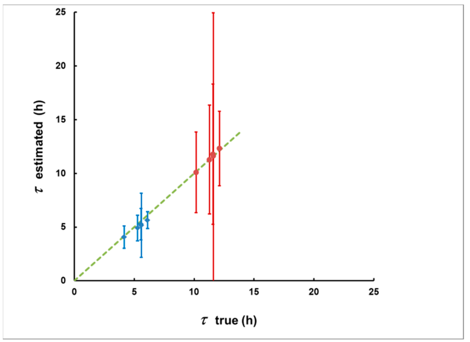
Figure 12.
The estimated delays and their uncertainties due to the “counting statistics” (error bars) for the five plumes from Figure 11 and with the two delay scenarios (the first is in blue, the second is in red). Notably, the methodological bias (the deviation of the points from the dashed line that corresponds to the coincidence of the estimated and true delay) is much smaller than the statistical uncertainty.

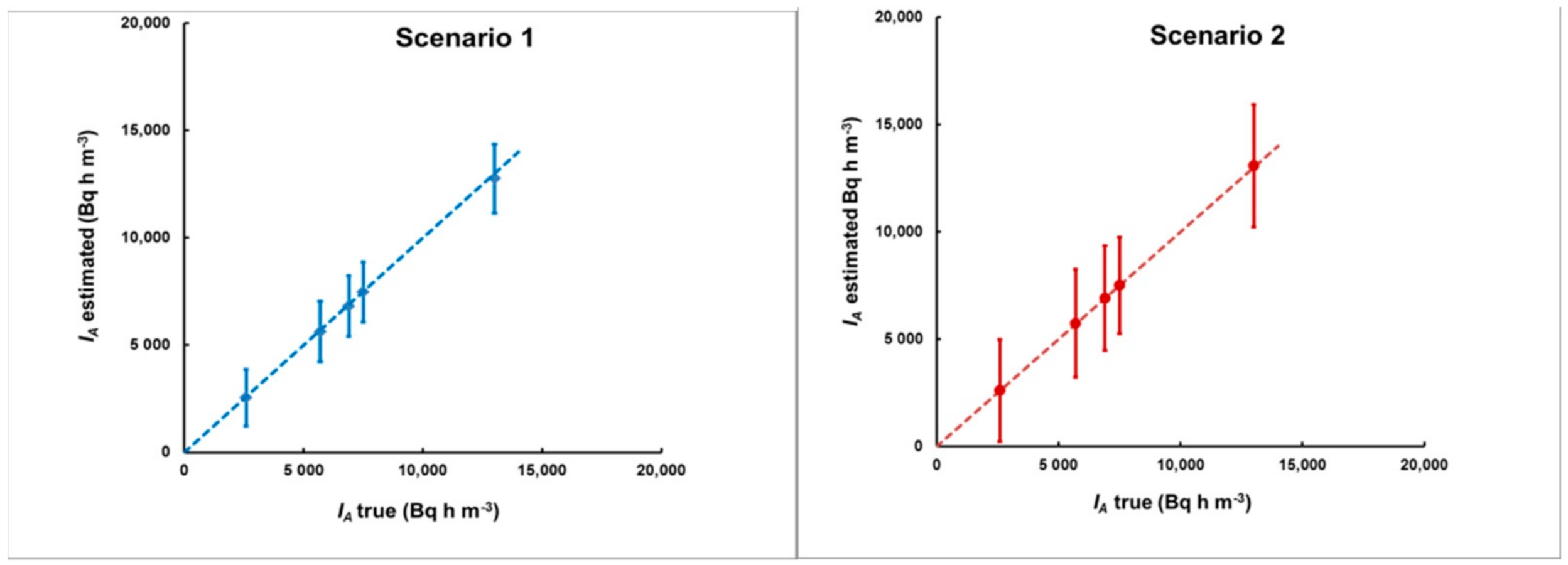
Figure 13.
The estimated integrated activity concentrations for the plumes of Figure 11 for the first (left) and the second (right) delay scenario. As with the delay estimates, here, the methodological bias (the deviation of the points from the dashed line that corresponds to “estimated = true IA”) is also much smaller than the “counting statistics uncertainty” (error bars).

Publisher’s Note: MDPI stays neutral with regard to jurisdictional claims in published maps and institutional affiliations. |
© 2021 by the authors. Licensee MDPI, Basel, Switzerland. This article is an open access article distributed under the terms and conditions of the Creative Commons Attribution (CC BY) license (https://creativecommons.org/licenses/by/4.0/).
Share and Cite
MDPI and ACS Style
Pressyanov, D.; Stavrev, P. A Method for Identification and Assessment of Radioxenon Plumes by Absorption in Polycarbonates. Sensors 2021, 21, 8107. https://0-doi-org.brum.beds.ac.uk/10.3390/s21238107
AMA Style
Pressyanov D, Stavrev P. A Method for Identification and Assessment of Radioxenon Plumes by Absorption in Polycarbonates. Sensors. 2021; 21(23):8107. https://0-doi-org.brum.beds.ac.uk/10.3390/s21238107
Chicago/Turabian StylePressyanov, Dobromir, and Pavel Stavrev. 2021. "A Method for Identification and Assessment of Radioxenon Plumes by Absorption in Polycarbonates" Sensors 21, no. 23: 8107. https://0-doi-org.brum.beds.ac.uk/10.3390/s21238107
Note that from the first issue of 2016, this journal uses article numbers instead of page numbers. See further details here.