
Performance Analysis of IoT and Long-Range Radio-Based Sensor Node and Gateway Architecture for Solid Waste Management

 , , , , , , and
Abstract
:1. Introduction
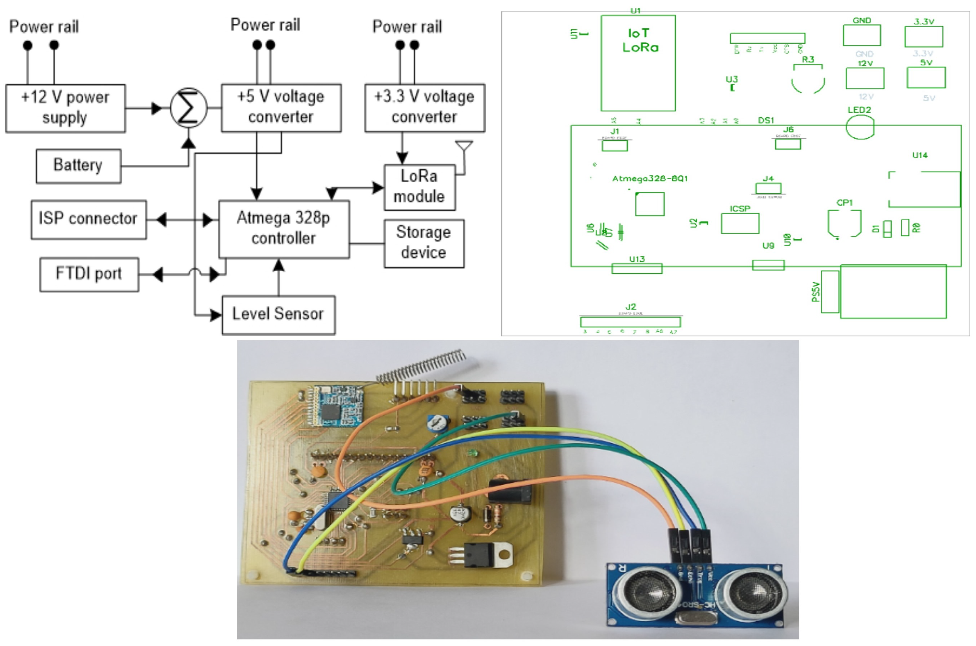
- We proposed architecture for designing and developing a customized sensor node and gateway based on LoRa technology for realizing the filling level of the bins with minimal energy consumption.
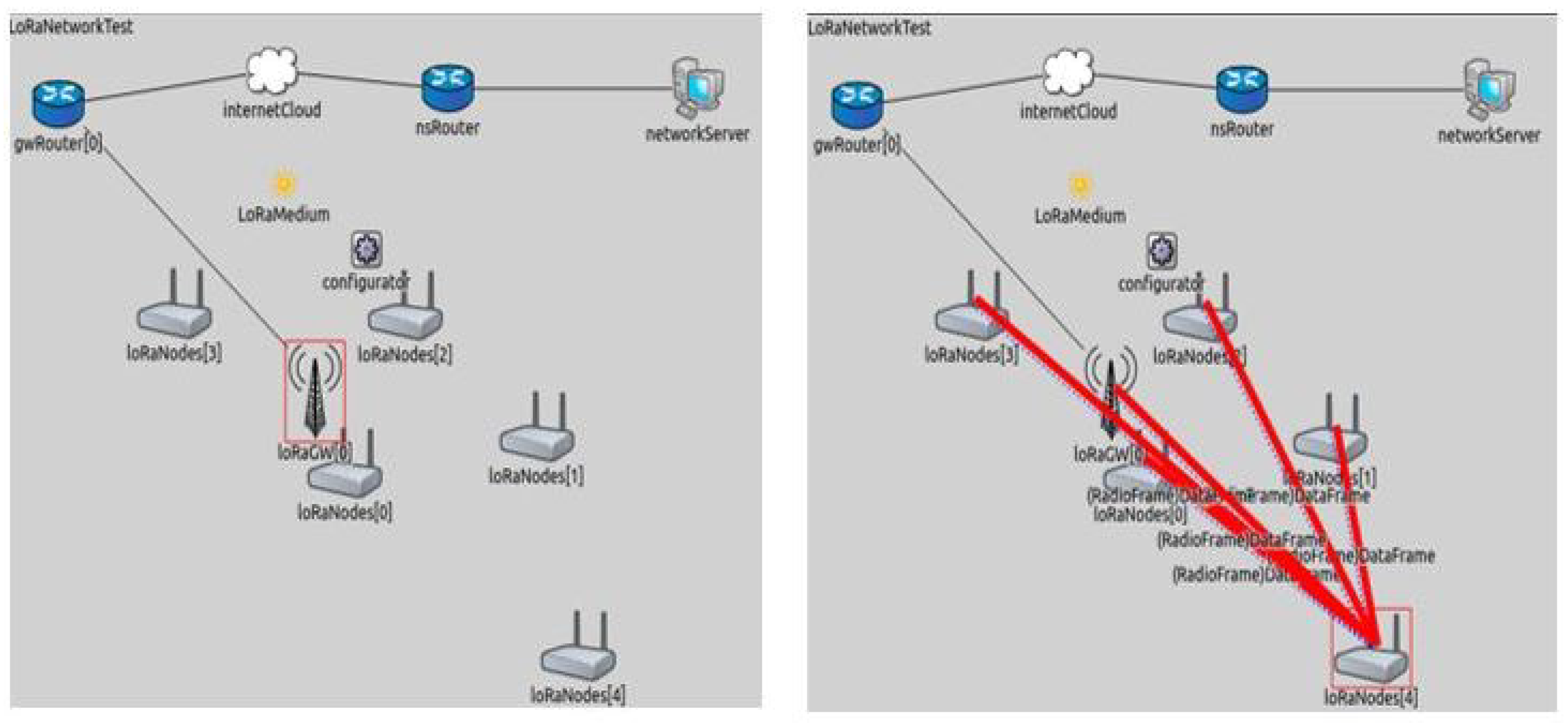
- We evaluated the energy consumption of the proposed architecture by simulating it on the Framework for LoRa (FLoRa) simulation by varying distinct fundamental parameters of LoRa communication.
- We provided the distinct evaluation metrics of the long-range data rate, time on-air (ToA), LoRa sensitivity, link budget, and battery life of sensor node.
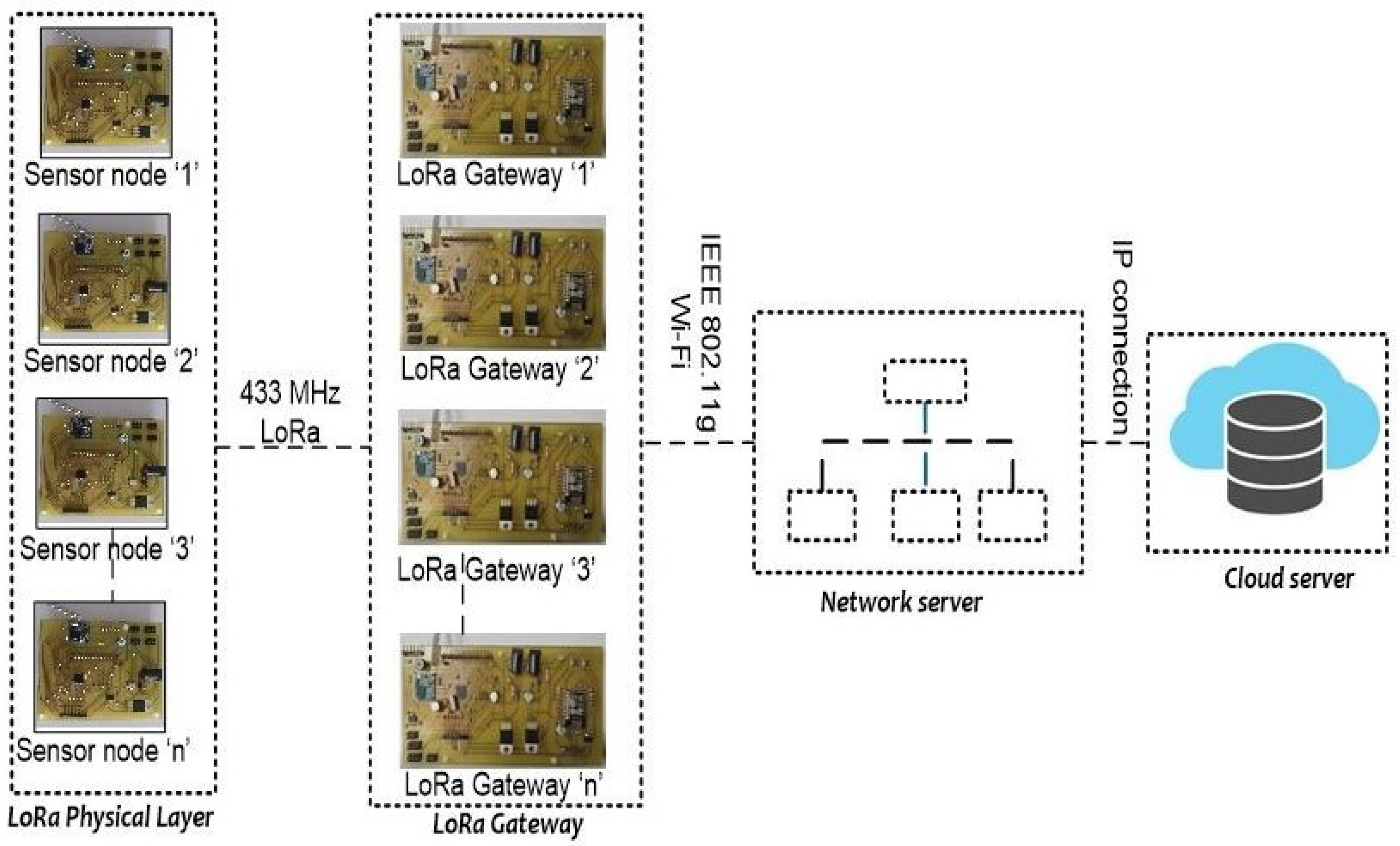
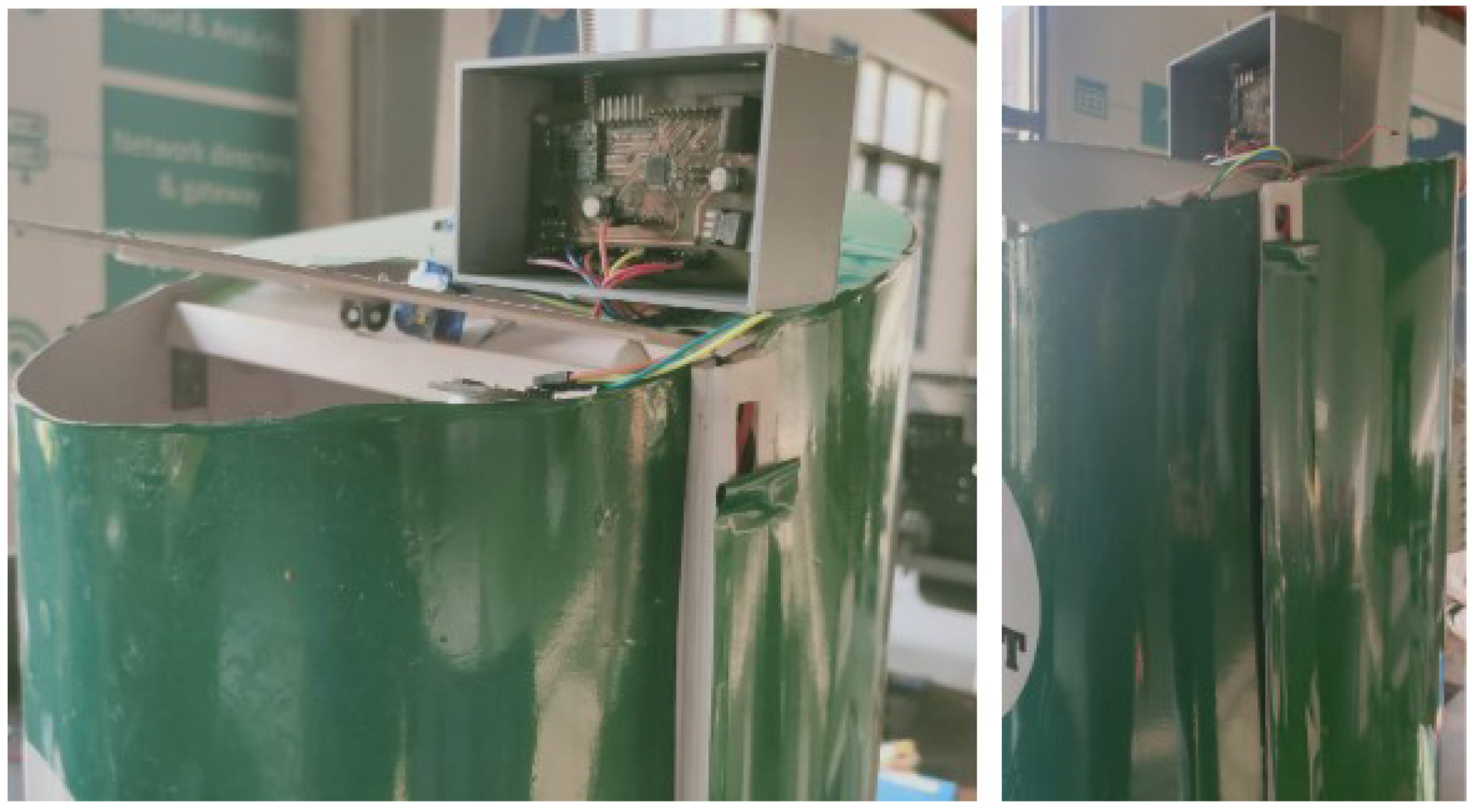
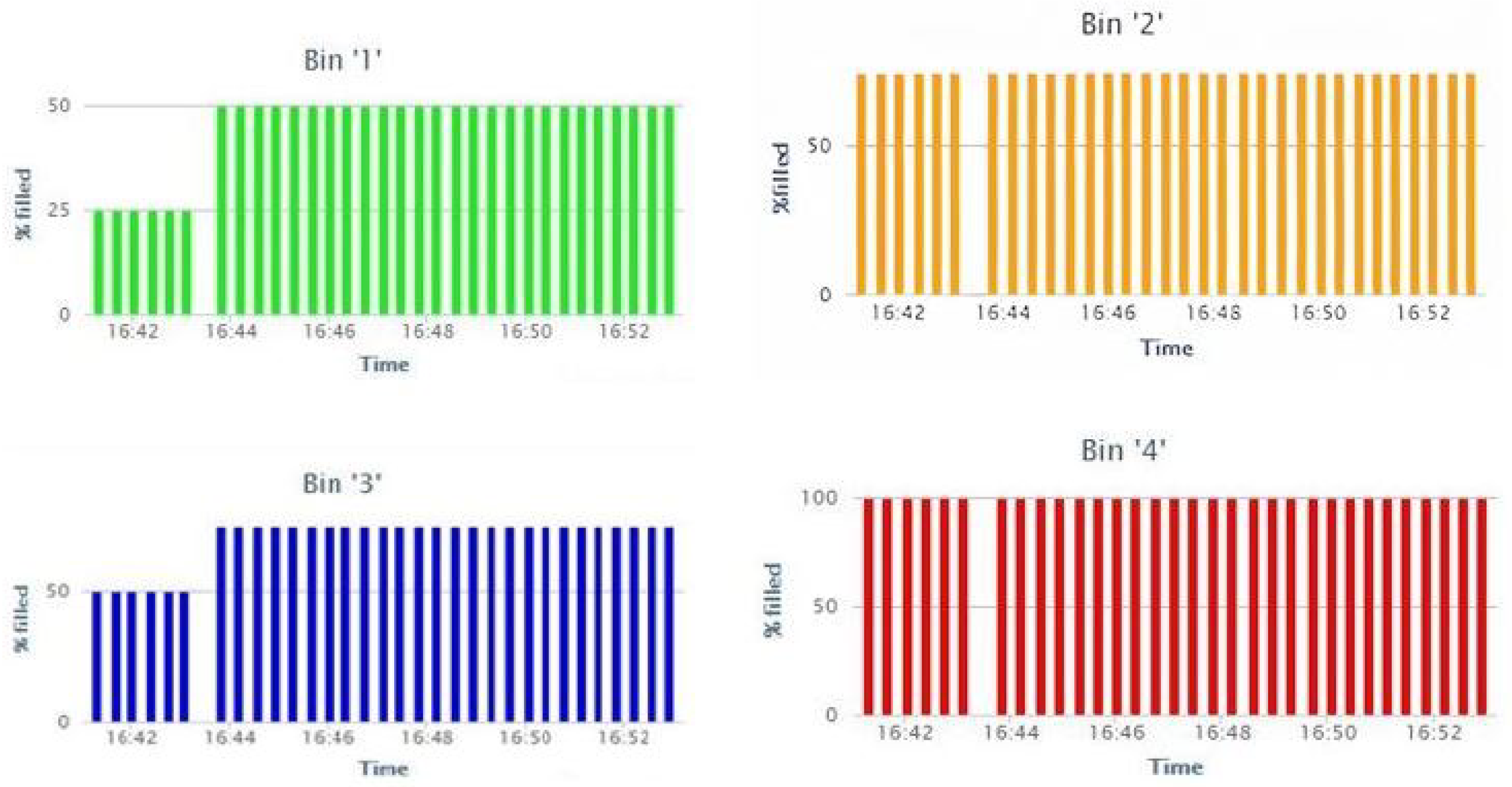
- We concluded with a real-time experimental setup, where we received the sensor data on the cloud server with a customized sensor node and gateway.
2. Related Work
3. Overview of LoRa
- SF is the number of chirps generated by each symbol, and its range is between 7 and 12. The higher the SF value, the better the receiver will eliminate the noise from the signal. The more time it takes to deliver a packet, the greater the amount it takes to transmit the packet.
- CF is the frequency of a carrier wave that is modulated to transmit signals; SX 1278 transceiver works on a carrier frequency of 433 MHz.
- BW depicts the frequency in the spectrum band, and it is chosen from these three bands: 500 kHz, 250 kHz, or 125 kHz. Large bandwidth represents speed transmission and the small bandwidth presents long-range transmission. The main parameter of the LoRa modulation is BW. The 2SF chirps that covers the entire frequency band is represented as LoRa symbol. Initially, it begins with a sequence of upward chirps, if the highest frequency band is achieved then frequency is wrapped and there will be a rise in the frequency again from the lowest frequency.
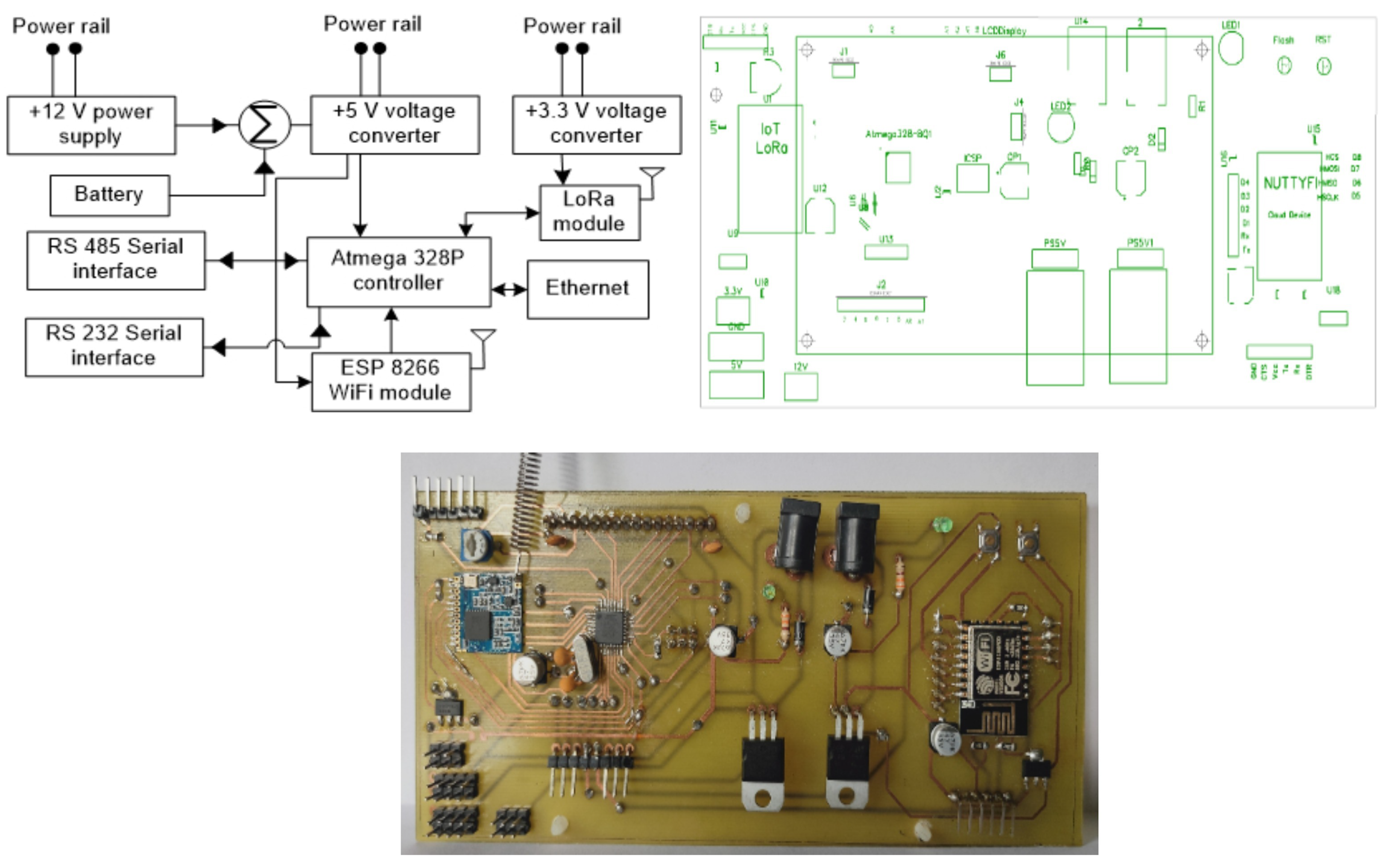
4. Hardware Implementation
5. LoRa Architecture for Waste Management
6. Performance Analysis
6.1. Energy Consumption of Nodes
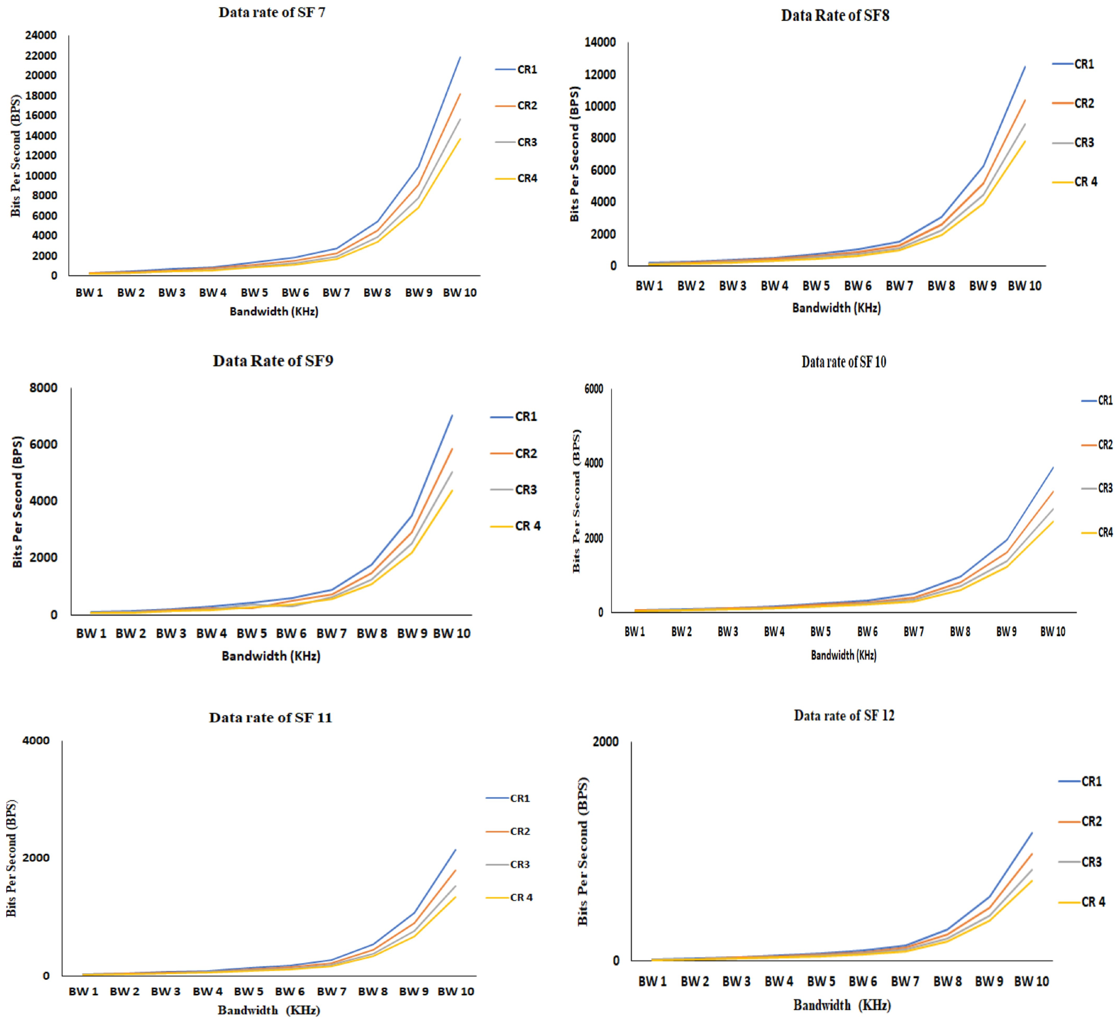
6.2. Data Rate/Bit Rate
6.3. LoRa Sensitivity
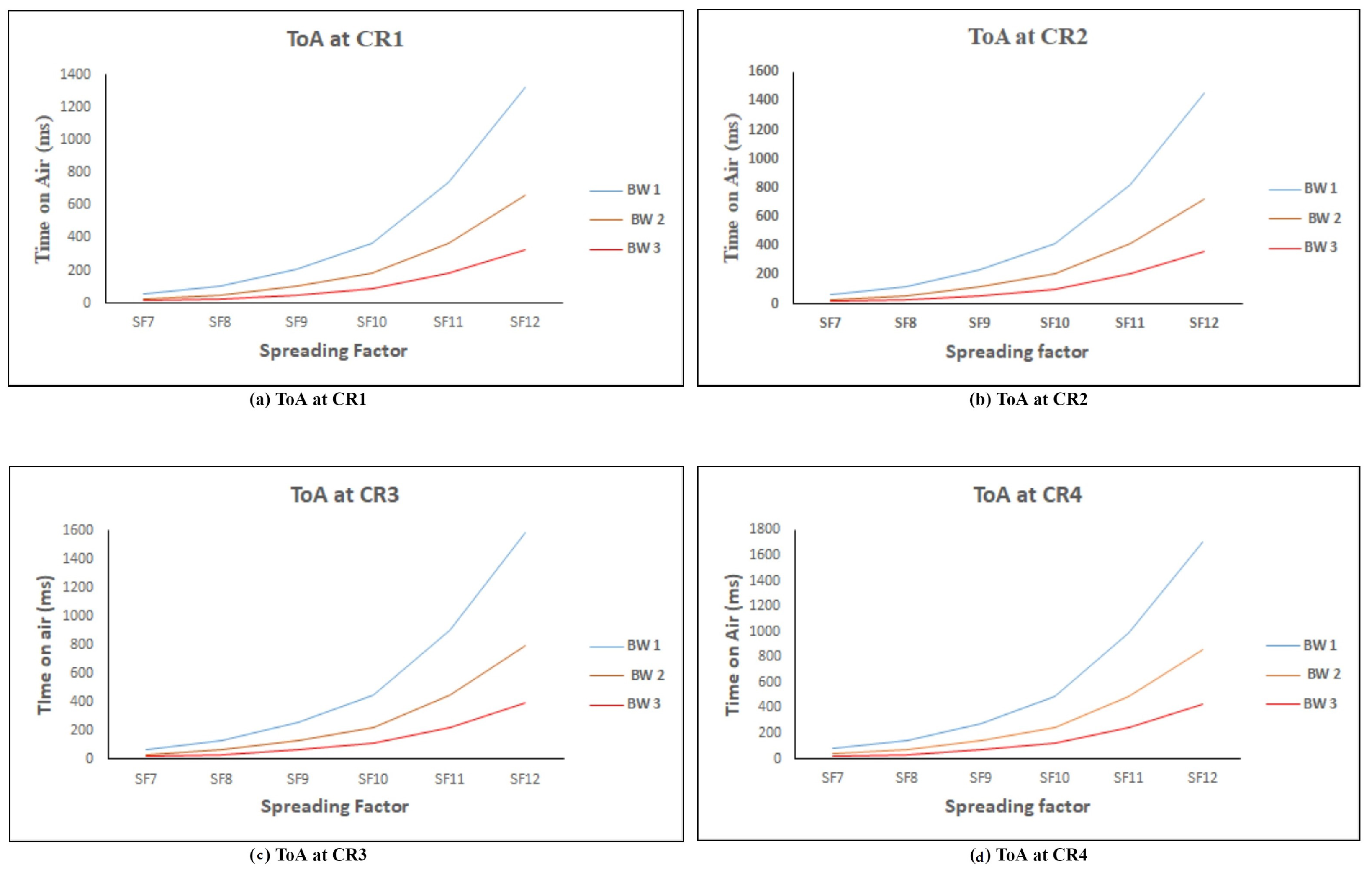
6.4. Time on Air (ToA)
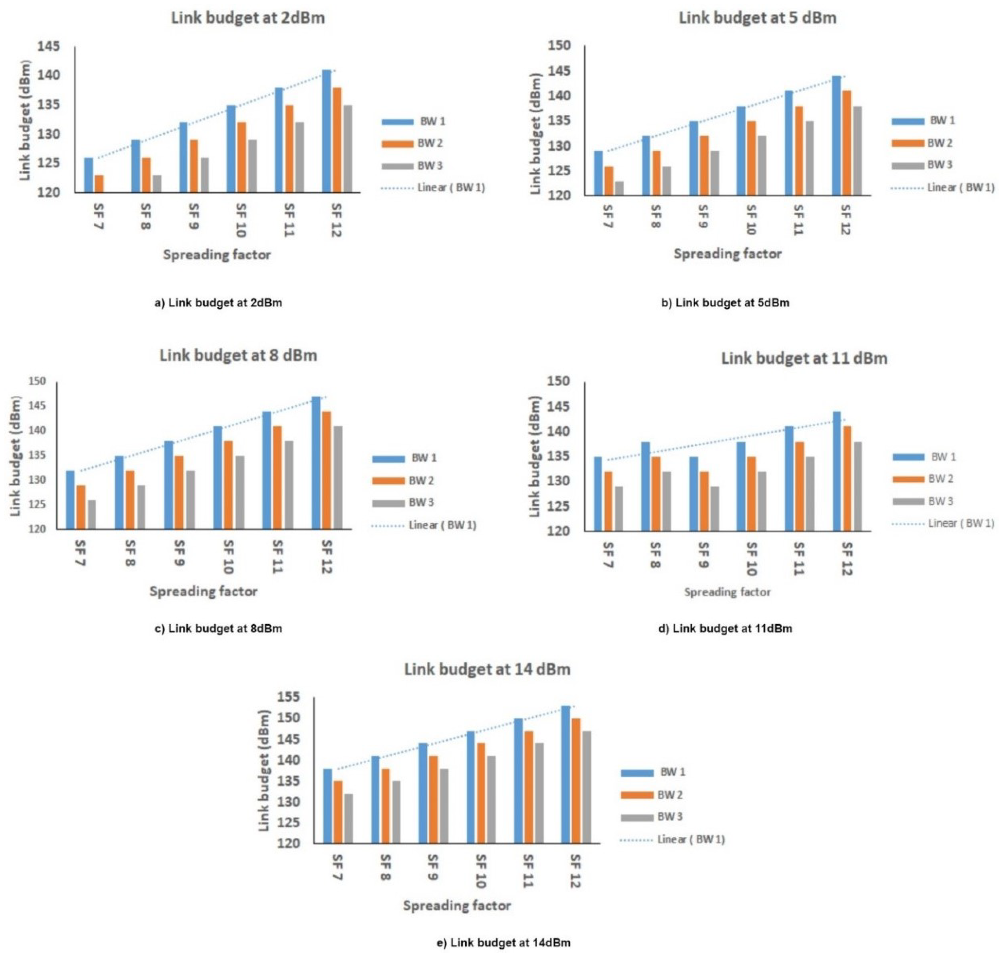
6.5. Link Budget
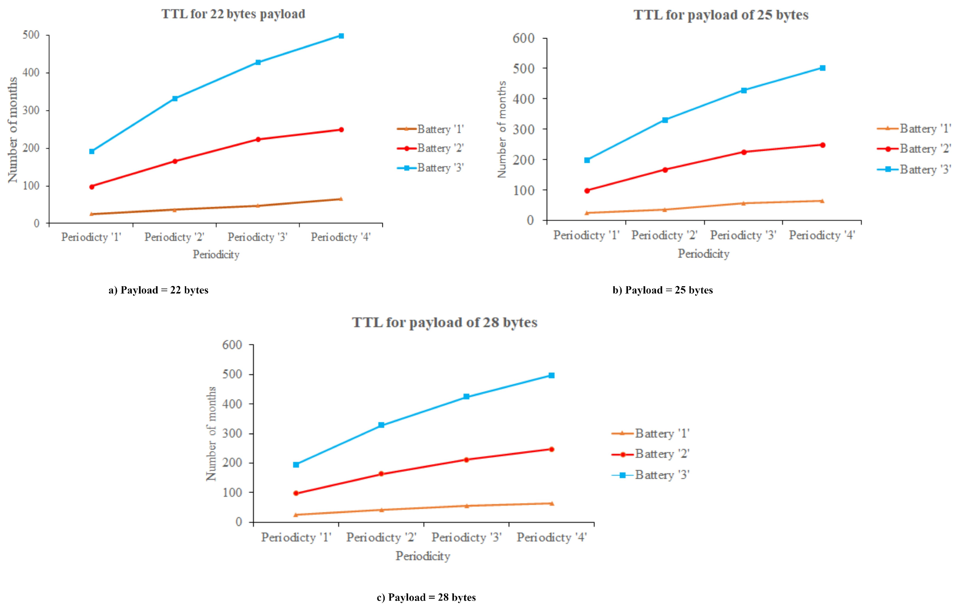
6.6. Battery Life of Sensor Node
7. Result Analysis
8. Conclusions
Author Contributions
Funding
Institutional Review Board Statement
Informed Consent Statement
Data Availability Statement
Conflicts of Interest
Abbreviations
| BW | Bandwidth |
| CF | Carrier Frequency |
| CR | Code Rate |
| CRC | Cyclic Redundancy Check |
| CSS | Chirp Spread Spectrum |
| FEC | Forward Error Correction |
| FLoRa | Framework for LoRa |
| FSPL | Free Space Path Loss |
| GSM | Global System for Mobile communication |
| GPRS | Global packet radio service |
| GPS | Global Positioning System |
| IEEE | Institute of Electrical and Electronics Engineers |
| IoT | Internet of Things |
| IP | Internet Protocol |
| LoRa | Long Range |
| LoRaWAN | LoRa Wide Area Network |
| MQTT | Message Queuing Telemetry Transport |
| PCB | Printed Circuit Board |
| RFID | Radio Frequency Identification |
| SF | Spreading Factor |
| SoC | System on a Chip |
| ToA | Time on Air |
| SNIR | Signal-to-Noise Ratio |
| VANET | Vehicular Ad Hoc Network |
| Wi-Fi | Wireless Fidelity |
| WSN | Wireless Sensor Network |
References
- THE 17 GOALS|Sustainable Development. Available online: https://sdgs.un.org/goals (accessed on 28 December 2020).
- Manager. The Weight of Cities. 2018. Available online: https://www.resourcepanel.org/reports/weight-cities (accessed on 1 January 2021).
- Kumar, S.; Smith, S.R.; Fowler, G.; Velis, C.; Kumar, S.J.; Arya, S.; Rena; Kumar, R.; Cheeseman, C. Challenges and opportunities associated with waste management in India. R. Soc. Open Sci. 2017, 4, 160764. [Google Scholar] [CrossRef] [PubMed] [Green Version]
- Sinha, R.S.; Wei, Y.; Hwang, S.-H. A survey on LPWA technology: LoRa and NB-IoT. ICT Express 2017, 3, 14–21. [Google Scholar] [CrossRef]
- Nižetić, S.; Šolić, P.; González-de-Artaza, D.L.; Patrono, L. Internet of Things (IoT): Opportunities, issues and challenges towards a smart and sustainable future. J. Clean. Prod. 2020, 274, 122877. [Google Scholar] [CrossRef] [PubMed]
- Kumar, S.; Jasuja, A. Air quality monitoring system based on IoT using Raspberry Pi. In Proceedings of the IEEE International Conference on Computing, Communication and Automation, ICCCA 2017, Greater Noida, India, 5–6 May 2017; Institute of Electrical and Electronics Engineers Inc.: Greater Noida, India, 2017; pp. 1341–1346. [Google Scholar]
- Gomez, C.; Chessa, S.; Fleury, A.; Roussos, G.; Preuveneers, D. Internet of Things for enabling smart environments: A technology-centric perspective. J. Ambient. Intell. Smart Environ. 2019, 11, 23–43. [Google Scholar] [CrossRef] [Green Version]
- Hussain, A.; Draz, U.; Ali, T.; Tariq, S.; Irfan, M.; Glowacz, A.; Daviu, J.A.A.; Yasin, S.; Rahman, S. Waste Management and Prediction of Air Pollutants Using IoT and Machine Learning Approach. Energies 2020, 13, 3930. [Google Scholar] [CrossRef]
- Jain, A.; Sharma, B.; Gupta, P. Internet of things: Architecture, security goals, and challenges—A survey. Int. J. Innov. Res. Sci. Eng. 2016, 2, 154–163. [Google Scholar]
- Longhi, S.; Marzioni, D.; Alidori, E.; Buo, G.D.; Prist, M.; Grisostomi, M.; Pirro, M. Solid waste management architecture using wireless sensor network technology. In Proceedings of the 2012 5th International Conference on New Technologies, Mobility and Security, Istanbul, Turkey, 7–10 May 2012; pp. 1–5. [Google Scholar]
- Dubey, S.; Singh, M.K.; Singh, P.; Aggarwal, S. Waste Management of Residential Society using Machine Learning and IoT Approach. In Proceedings of the International Conference Emerging Smart Computing and Informatics, ESCI 2020, Pune, India, 12–14 March 2020; pp. 293–297. [Google Scholar]
- Madakam, S.; Ramaswamy, R.; Tripathi, S. Internet of Things (IoT): A Literature Review. J. Comput. Commun. 2015, 3, 164–173. [Google Scholar] [CrossRef] [Green Version]
- Mekki, K.; Bajic, E.; Chaxel, F.; Meyer, F. A comparative study of LPWAN technologies for large-scale IoT deployment. ICT Express. 2019, 5, 1–7. [Google Scholar] [CrossRef]
- Sheng, T.J.; Islam, M.S.; Misran, N.; Baharuddin, M.H.; Arshad, H.; Islam, M.R.; Chowdhury, M.E.H.; Rmili, H.; Islam, M.T. An internet of things based smart waste management system using LoRa and tensorflow deep learning model. IEEE Access. 2020, 8, 148793–148811. [Google Scholar] [CrossRef]
- Lokhande, P.; Pawar, M.D. Garbage Collection Management System. Int. J. Eng. Comput. Sci. 2016, 5, 18800–18805. [Google Scholar] [CrossRef]
- Kumar, G.N.; Swamy, C.; Nagadarshini, K.N. Efficient garbage disposal management in metropolitan cities using VANETs. J. Clean Energy Technol. 2014, 2, 258–262. [Google Scholar]
- Lata, K.; Singh, S.S.K. IOT based smart waste management system using Wireless Sensor Network and Embedded Linux Board. Int. J. Curr. Trends Eng. Res. 2016, 2, 210–214. [Google Scholar]
- Omara, A.; Gulen, D.; Kantarci, B.; Oktug, S.F. Trajectory-Assisted Municipal Agent Mobility: A Sensor-Driven Smart Waste Management System. J. Sens. Actuator Netw. 2018, 7, 29. [Google Scholar] [CrossRef] [Green Version]
- Suryawanshi, S.; Bhuse, R.; Gite, M.; Hande, D. Waste Management System Based On IoT. Int. Res. J. Eng. Technol. 2018, 5, 1835–1837. [Google Scholar]
- Cavdar, K.; Koroglu, M.; Akyildiz, B. Design and implementation of a smart solid waste collection system. Int. J. Environ. Sci. Technol. 2016, 13, 1553–1562. [Google Scholar] [CrossRef] [Green Version]
- Karthikeyan, S.; Rani, G.S.; Sridevi, M.; Bhuvaneswari, P.T.V. IoT enabled waste management system using ZigBee network. In Proceedings of the 2nd IEEE International Conference Recent Trends ELECTRONICS Information and Communication Technology, Bangalore, India, 19–20 May 2017; pp. 2182–2187. [Google Scholar]
- Reis, P.; Caetano, F.; Pitarma, R.; Gonçalves, C. IEcoSys—An intelligent waste management system. In Advances in Intelligent Systems and Computing; Springer: Berlin/Heidelberg, Germany, 2015; pp. 843–853. [Google Scholar]
- Satria, D.; Hidayat, T. Implementation of wireless sensor network (WSN) on garbage transport warning information system using GSM module. J. Phys. Conf. Ser. 2019, 1175, 12054. [Google Scholar] [CrossRef]
- Zavare, S.; Parashare, R.; Patil, S.; Rathod, P.; Babanne, V. Smart City waste management system using GSM. Int. J. Comput. Sci. Trends Technol. 2017, 5, 74–78. [Google Scholar]
- Augustin, A.; Yi, J.; Clausen, T.; Townsley, W.M. A study of Lora: Long range & low power networks for the internet of things. Sensors 2016, 16, 1466. [Google Scholar]
- Saari, M.; bin Baharudin, A.M.; Sillberg, P.; Hyrynsalmi, S.; Yan, W. LoRa—A survey of recent research trends. In Proceedings of the 41st International Convention on Information and Communication Technology, Electronics and Microelectronics (MIPRO), Opatija, Croatia, 21–25 May 2018; pp. 872–877. [Google Scholar]
- Lozano, Á.; Caridad, J.; Paz, J.F.D.; González, G.V.; Bajo, J. Smart waste collection system with low consumption LoRaWAN nodes and route optimization. Sensors 2018, 18, 1465. [Google Scholar] [CrossRef] [Green Version]
- Cerchecci, M.; Luti, F.; Mecocci, A.; Parrino, S.; Peruzzi, G.; Pozzebon, A. A low power IoT sensor node architecture for waste management within smart cities context. Sensors 2018, 18, 1282. [Google Scholar] [CrossRef] [Green Version]
- Addabbo, T.; Fort, A.; Mecocci, A.; Mugnaini, M.; Parrino, S.; Pozzebon, A.; Vignoli, V. A LoRa-based IoT Sensor Node for Waste Management Based on a Customized Ultrasonic Transceiver. In Proceedings of the IEEE Sensors Applications Symposium, Sophia Antipolis, France, 11–13 March 2019; pp. 1–6. [Google Scholar]
- Lavric, A.; Petrariu, A.I.; Coca, E.; Popa, V. Lora traffic generator based on software defined radio technology for lora modulation orthogonality analysis: Empirical and experimental evaluation. Sensors 2020, 20, 4123. [Google Scholar] [CrossRef] [PubMed]
- Semtech Corporation. SX1272/3/6/7/8 LoRa Modem Design Guide, AN1200.13. 2013, p. 9. Available online: https://www.rs-online.com/ (accessed on 7 March 2021).
- Ortín, J.; Cesana, M.; Redondi, A. How do ALOHA and listen before talk coexist in LoRaWAN? In Proceedings of the IEEE 29th Annual International Symposium on Personal, Indoor and Mobile Radio Communications, Bologna, Italy, 9–12 September 2018; pp. 1–7. [Google Scholar]
- Balanis, C.A. Antenna Theroy: Analysis and Design; John Wiley & Sons: Hoboken, NJ, USA, 2012; p. 109. [Google Scholar]
- Sendra, S.; García, L.; Lloret, J.; Bosch, I.; Vega-Rodríguez, R. LoRaWAN network for fire monitoring in rural environments. Electronics 2020, 9, 531. [Google Scholar] [CrossRef] [Green Version]
- Semtech Corporation. SX1276/77/78/79—137 MHz to 1020 MHz Low Power Long Range Transceiver. 2016. Available online: https://www.scribd.com/document/399165229/SX1276-1278 (accessed on 7 March 2021).
- Atmel Corporation. Data Sheet ATmega328P. 2015, pp. 1–294. Available online: http://ww1.microchip.com/downloads/en/DeviceDoc/Atmel-7810-Automotive-Microcontrollers-ATmega328P_Datasheet.pdf (accessed on 9 March 2021).
- ESP8266 Wi-Fi MCU I Espressif Systems. 2020. Available online: https://www.espressif.com/en/products/socs/esp8266 (accessed on 9 March 2021).
- Magrin, D.; Centenaro, M.; Vangelista, L. Performance evaluation of LoRa networks in a smart city scenario. In Proceedings of the IEEE International Conference on Communications, Paris, France, 21–25 May 2017; pp. 1–7. [Google Scholar]
- OMNeT++ Discrete Event Simulator. Available online: https://omnetpp.org/ (accessed on 18 February 2021).
- Home|FLoRa—A Framework for LoRa Simulations. Available online: https://flora.aalto.fi/ (accessed on 18 February 2021).
- Slabicki, M.; Premsankar, G.; Francesco, M.D. Adaptive configuration of LoRa networks for dense IoT deployments. In Proceedings of the NOMS 2018–2018 IEEE/IFIP Network Operations and Management Symposium, Taipei, Taiwan, 23–27 April 2018; pp. 1–9. [Google Scholar]
- Petajajarvi, J.; Mikhaylov, K.; Roivainen, A.; Hanninen, T.; Pettissalo, M. On the coverage of LPWANs: Range evaluation and channel attenuation model for LoRa technology. In Proceedings of the 14th International Conference on ITS Telecommunications, Copenhagen, Denmark, 2–4 December 2015; pp. 55–59. [Google Scholar]
- LoRaTool. Available online: https://www.loratools.nl (accessed on 1 April 2021).
- Lundin, A.C.; Ozkil, A.G.; Schuldt-Jensen, J. Smart cities A case study in waste monitoring and management. In Proceedings of the 50th Hawaii International Conference on System Sciences, Waikoloa, HI, USA, 4–7 January 2017; pp. 1392–1401. [Google Scholar]
- Ziouzios, D.; Dasygenis, M. A smart bin implementantion using LoRa. In Proceedings of the 2019 4th South-East Europe Design Automation, Computer Engineering, Computer Networks and Social Media Conference (SEEDA-CECNSM 2019), Piraeus, Greece, 20–22 September 2019; Institute of Electrical and Electronics Engineers Inc.: Piraeus, Greece, 2019. [Google Scholar]
- Beliatis, M.J.; Mansour, H.; Nagy, S.; Aagaard, A.; Presser, M. Digital waste management using LoRa network a business case from lab to fab. In Proceedings of the Global Internet Things Summit, GIoTS 2018, Bilbao, Spain, 4–7 June 2018; pp. 1–6. [Google Scholar]
- Khoa, T.A.; Phuc, C.H.; Lam, P.D.; Nhu, L.M.B.; Trong, N.M.; Phuong, N.T.H.; Dung, N.V.; Nguyen, N.; Ta, H.N.; Duc, D.N.M. Waste Management System Using IoT-Based Machine Learning in University. Wirel. Commun. Mob. Comput. 2020, 2020, 6138637. [Google Scholar]


| Characteristic | Specification |
|---|---|
| Frequency | 433 MHz |
| Network topology | Point-to-Multipoint, Point-to-Point, Mesh, and Peer-to-Peer |
| Modulation | FSK/GFSK/MSK/LoRa |
| Data rate | <300 kbps |
| Sensitivity | −136 dBm |
| Output power | +20 dB |
| Operating voltage | 1.8 V to 3.6 V |
| Current | Tx: 120 mA, Rx: 10.8 mA |
| RSSI | 127 dB |
| Link budget | 168 dB |
| Characteristic | Specification |
|---|---|
| Controller | 8-bit microcontroller |
| Architecture | RISC |
| Programming | In-system programming |
| Serial interface | Master/slave SPI |
| PWM channels | 6 |
| Pin 6 analog pins | 14 digital pins |
| Operating voltage | 2.7 V to 5.5 V |
| Current | Active state: 1.5 mA at 3 V–4 MHz, |
| Power-down state: 1 µA at 3 V |
| Parameter | Feature |
|---|---|
| Processor | Tensilica L106 32-bit processor |
| IEEE standard | 802.11 b/g/n |
| Frequency | 2.4 GHz |
| Data rate | 72 Mbps |
| Network Protocols | Ipv4, TCP/UDP, HTTP |
| Tx power | 20 dBm (802.11 b), 17 dBm (802.11 g) & 14 dBm (802.11 n) |
| Rx sensitivity | −91 dBm (802.11 b), −75 dBm (802.11 g) & −71 dBm (802.11 n) |
| Operating voltage | 2.5 V to 3.6 V |
| Current | Average: 80 mA |
| Node | Tx Power = 2 dBm | Tx Power = 5 dBm | Tx Power = 8 dBm | Tx Power = 11 dBm | Tx Power = 14 dBm |
|---|---|---|---|---|---|
| 1 | 2.45 mW | 2.46 mW | 2.46 mW | 2.09 mW | 2.18 mW |
| 2 | 2.45 mW | 2.46 mW | 2.18 mW | 1.9 mW | 2.03 mW |
| 3 | 1.89 mW | 1.90 mW | 2.74 mW | 3.10 mW | 3.24 mW |
| 4 | 2.38 mW | 2.39 mW | 2.60 mW | 2.31 mW | 2.41 mW |
| Node | Tx Power = 2 dBm | Tx Power = 5 dBm | Tx Power = 8 dBm | Tx Power = 11 dBm | Tx Power = 14 dBm |
|---|---|---|---|---|---|
| 1 | 1.68 mW | 1.69 mW | 2.39 mW | 2.10 mW | 2.78 mW |
| 2 | 2.10 mW | 2.11 mW | 2.53 mW | 2.81 mW | 2.03 mW |
| 3 | 2.10 mW | 2.12 mW | 2.60 mW | 2.52 mW | 2.63 mW |
| 4 | 2.24 mW | 2.25 mW | 2.39 mW | 2.24 mW | 3.69 mW |
| Node | Tx Power = 2 dBm | Tx Power = 5 dBm | Tx Power = 8 dBm | Tx Power = 11 dBm | Tx Power = 14 dBm |
|---|---|---|---|---|---|
| 1 | 1.75 mW | 1.76 mW | 2.04 mW | 3.25 mW | 1.95 mW |
| 2 | 1.61 mW | 1.59 mW | 2.32 mW | 1.95 mW | 1.88 mW |
| 3 | 3.01 mW | 3.02 mW | 2.88 mW | 1.95 mW | 1.88 mW |
| 4 | 2.52 mW | 2.53 mW | 2.11 mW | 2.38 mW | 1.88 mW |
| 5 | 2.03 mW | 2.04 mW | 2.04 mW | 2.09 mW | 2.48 mW |
| 6 | 2.51 mW | 2.46 mW | 2.74 mW | 2.74 mW | 2.48 mW |
| 7 | 2.17 mW | 2.18 mW | 1.83 mW | 2.74 mW | 2.33 mW |
| 8 | 1.96 mW | 1.97 mW | 2.11 mW | 2.31 mW | 2.56 mW |
| Node | Tx Power = 2 dBm | Tx power =5 dBm | Tx Power = 8 dBm | Tx Power = 11 dBm | Tx Power = 14 dBm |
|---|---|---|---|---|---|
| 1 | 2.11 mW | 2.11 mW | 2.53 mW | 2.81 mW | 2.71 mW |
| 2 | 1.96 mW | 1.97 mW | 2.26 mW | 2.46 mW | 2.26 mW |
| 3 | 1.82 mW | 1.83 mW | 2.81 mW | 2.09 mW | 2.86 mW |
| 4 | 2.66 mW | 2.67 mW | 3.17 mW | 2.31 mW | 2.71 mW |
| 5 | 1.89 mW | 1.90 mW | 1.89 mW | 2.46 mW | 3.08 mW |
| 6 | 2.38 mW | 2.39 mW | 2.39 mW | 2.09 mW | 1.88 mW |
| 7 | 2.31 mW | 2.32 mW | 2.53 mW | 1.96 mW | 2.86 mW |
| 8 | 2.09 mW | 2.04 mW | 2.32 mW | 2.74 mW | 2.26 mW |
| 9 | 1.89 mW | 1.90 mW | 3.10 mW | 2.60 mW | 3.31 mW |
| 10 | 2.60 mW | 2.61 mW | 2.67 mW | 2.64 mW | 1.73 mW |
| 11 | 2.03 mW | 2.04 mW | 2.60 mW | 2.45 mW | 2.18 mW |
| 12 | 1.75 mW | 1.76 mW | 1.90 mW | 2.60 mW | 2.03 mW |
| 13 | 2.80 mW | 2.81 mW | 1.76 mW | 3.10 mW | 2.78 mW |
| 14 | 1.96 mW | 1.97 mW | 2.74 mW | 2.09 mW | 2.63 mW |
| 15 | 2.03 mW | 1.97 mW | 2.46 mW | 2.52 mW | 2.48 mW |
| 16 | 2.38 mW | 2.39 mW | 2.82 mW | 2.81 mW | 2.33 mW |
| SF | BW 1 = 125 KHz | BW 2 = 250 KHz | BW 3 = 500 KHz |
|---|---|---|---|
| SF 7 | 56.58 | 28.29 | 14.14 |
| SF 8 | 102.91 | 51.46 | 25.73 |
| SF 9 | 205.82 | 102.91 | 51.46 |
| SF 10 | 370.69 | 185.34 | 92.67 |
| SF 11 | 741.38 | 370.69 | 185.34 |
| SF 12 | 1318.91 | 659.46 | 329.73 |
| SF | BW 1 = 125 KHz | BW 2 = 250 KHz | BW 3 = 500 KHz |
|---|---|---|---|
| SF 7 | 63.74 | 31.87 | 15.94 |
| SF 8 | 115.2 | 57.6 | 28.8 |
| SF 9 | 230.4 | 115.2 | 57.6 |
| SF 10 | 411.65 | 205.82 | 102.91 |
| SF 11 | 823.3 | 411.65 | 205.82 |
| SF 12 | 1449.98 | 724.99 | 362.5 |
| SF | BW 1 = 125 KHz | BW 2 = 250 KHz | BW 3 = 500 KHz |
|---|---|---|---|
| SF 7 | 70.91 | 35.46 | 17.73 |
| SF 8 | 127.49 | 63.74 | 31.87 |
| SF 9 | 254.98 | 127.49 | 63.74 |
| SF 10 | 452.61 | 226.3 | 113.15 |
| SF 11 | 905.22 | 452.61 | 226.3 |
| SF 12 | 1581.06 | 790.53 | 395.26 |
| SF | BW 1 = 125 KHz | BW 2 = 250 KHz | BW 3 = 500 KHz |
|---|---|---|---|
| SF 7 | 78.08 | 39.04 | 19.52 |
| SF 8 | 139.78 | 69.89 | 34.94 |
| SF 9 | 279.55 | 139.78 | 69.89 |
| SF 10 | 493.57 | 246.78 | 123.39 |
| SF 11 | 987.14 | 493.57 | 246.78 |
| SF 12 | 1712.13 | 856.06 | 428.03 |
| Research | MCU | Communication | Designed Sensor Node | Designed Gateway | Customized Node | Proof of Concept | Simulation- Based Analysis | Plot of Evaluation Metrics |
|---|---|---|---|---|---|---|---|---|
| [14] | Arduino Uno | SX 1272 LoRa & Waspmote | Yes | No | Yes | Yes | No | No |
| [27] | ATSAML21 | SX 1276 LoRa | Yes | No | Yes | Yes | No | No |
| [28] | Atmega328P | SX 1278 LoRa | Yes | No | Yes | Yes | No | No |
| [29] | Atmega328P | SX 1272 LoRa | Yes | No | Yes | Yes | No | No |
| [44] | NA | NA | Yes | No | No | Yes | No | No |
| [45] | Arduino Uno | SX 1272 LoRa | No | No | No | No | No | No |
| [46] | Raspberry Pi3 | IP67 LoRa gateway | No | Yes | Yes | Yes | No | No |
| [47] | Atmega328P | SX 1278 LoRa | Yes | Yes | Yes | Yes | No | No |
| Proposed study | Atmega328P | SX 1278 LoRa | Yes | Yes | Yes | Yes | Yes | Yes |
| S.No | Parameters | Achievements |
|---|---|---|
| 1 | Energy consumption | Energy consumption of nodes are calculated in FLoRa simulation by changing distinct network parameters |
| 2 | Data rate | An increase in SF leads to transmission of a low data rate, so SF 7 is the optimal for sending a large amount of the data. |
| 3 | Sensitivity power | The sensitivity power is highest for the SF 7 at the 500 kHz. |
| 4 | ToA | ToA is good at 125 KHz and code rate 1, i.e., 56.58 ms. |
| 5 | Link budget | At 14 dBm, 125 kHz and SF 12, maximum link budget is achieved. |
| 6 | Battery life of sensor node | Periodicity of transmitting data = 60 min, the bat- tery life is long, if Periodicity of transmitting data = 15 min, the battery life is short. |
| 7 | Real time experiment set up | Realized the objective of proposed architecture in Figure 4, where the sensor data is logging into the cloud server through the customized sensor node and gateway. |
Publisher’s Note: MDPI stays neutral with regard to jurisdictional claims in published maps and institutional affiliations. |
© 2021 by the authors. Licensee MDPI, Basel, Switzerland. This article is an open access article distributed under the terms and conditions of the Creative Commons Attribution (CC BY) license (https://creativecommons.org/licenses/by/4.0/).
Share and Cite
Akram, S.V.; Singh, R.; AlZain, M.A.; Gehlot, A.; Rashid, M.; Faragallah, O.S.; El-Shafai, W.; Prashar, D. Performance Analysis of IoT and Long-Range Radio-Based Sensor Node and Gateway Architecture for Solid Waste Management. Sensors 2021, 21, 2774. https://0-doi-org.brum.beds.ac.uk/10.3390/s21082774
Akram SV, Singh R, AlZain MA, Gehlot A, Rashid M, Faragallah OS, El-Shafai W, Prashar D. Performance Analysis of IoT and Long-Range Radio-Based Sensor Node and Gateway Architecture for Solid Waste Management. Sensors. 2021; 21(8):2774. https://0-doi-org.brum.beds.ac.uk/10.3390/s21082774
Chicago/Turabian StyleAkram, Shaik Vaseem, Rajesh Singh, Mohammed A. AlZain, Anita Gehlot, Mamoon Rashid, Osama S. Faragallah, Walid El-Shafai, and Deepak Prashar. 2021. "Performance Analysis of IoT and Long-Range Radio-Based Sensor Node and Gateway Architecture for Solid Waste Management" Sensors 21, no. 8: 2774. https://0-doi-org.brum.beds.ac.uk/10.3390/s21082774