Probabilistic Seismic Response Prediction of Three-Dimensional Structures Based on Bayesian Convolutional Neural Network

Abstract

Seismic response prediction is a challenging problem and is significant in every stage during a structure’s life cycle. Deep neural network has proven to be an efficient tool in the response prediction of structures. However, a conventional neural network with deterministic parameters is unable to predict the random dynamic response of structures. In this paper, a deep Bayesian convolutional neural network is proposed to predict seismic response. The Bayes-backpropagation algorithm is applied to train the proposed Bayesian deep learning model. A numerical example of a three-dimensional building structure is utilized to validate the performance of the proposed model. The result shows that both acceleration and displacement responses can be predicted with a high level of accuracy by using the proposed method. The main statistical indices of prediction results agree closely with the results from finite element analysis. Furthermore, the influence of random parameters and the robustness of the proposed model are discussed.

1. Introduction

An earthquake is a natural disaster which causes catastrophic damage to structures [1,2]. To accurately compute the seismic dynamic response and evaluate the safety of structures, the randomness and uncertainty of structure parameters need to be taken into consideration [3,4,5,6,7,8]. To solve this problem, various methods have been proposed by researchers since the 1960s, such as the Monte-Carlo simulation [9,10], the orthogonal polynomial expansion method [11] and the probability density evolution method [12,13,14,15]. The analytic results using these methods are given in the form of probability distributions. However, for these methods, the random parameter probability distributions need to be obtained before the calculation. If the probability distributions are unknown or change, these methods are difficult to carry out.

Recently, the development of neural network and deep learning [16] has provided a powerful approach for seismic response prediction. Different types of neural networks or deep learning models are currently used to predict the dynamic response of structures. The earliest work utilizing this approach aimed at response analysis of the linear response of structures, without considering any inherent uncertainty or randomness, and the types of neural network models were limited to multi-layer feedforward neural network (multilayer perceptron) [17,18,19,20]. To solve the problem of structural nonlinearity, prior knowledge was introduced into the neural network [21,22,23] and several new types of neural networks were proposed. With improvement of computational efficiency, deep learning models, such as deep convolutional neural network [24,25,26], deep recurrent neural network [26,27,28,29] and deep convolutional recurrent neural network [30], were developed and applied for structural seismic response prediction. Currently, wind-induced and vehicle-induced dynamic response predictions have attracted attention. Wang et al. used the deep recurrent neural network in structural response prediction under wind load [31]. Li et al. utilized the deep long- and short-time memory models for dynamic response prediction of a train-bridge system [32]. The probability-based method is combined with neural network and provides a new tool for random seismic response analysis. Kim used deep convolution neural networks to predict the peak and characteristic value of structural dynamic response under random earthquake [33]. Li et al. used the Bayesian deep learning model to predict the response of vehicle-bridge systems [34]. Wang et al. applied the Bayesian neural network in the seismic response prediction of single-degree of freedom (SDOF) systems [35]. However, so far, research work on seismic response prediction of three-dimensional buildings, with random characteristics, has been very limited.

In this paper, a Bayesian deep learning model [36] with convolutional neural network is utilized to predict the seismic response of a 3D building with random characteristics. The Bayes backprop algorithm as a high efficiency training algorithm, used to train the deep learning model. The trained model is utilized to predict the random response of a 3D building and to obtain the probability distribution of both displacement and acceleration responses. Finally, the influence of random parameters and the robustness of the proposed Bayesian deep learning model are discussed. The organization of this paper is as follows: In Section 2, the Bayesian deep learning theory and Bayes backprop algorithm are introduced; Section 3 provides the details of the numerical example of a 3D building with random characteristics; Section 4 presents the training process of the proposed deep learning model and illustrates the response prediction results for the 3D building; In Section 5, the influence of structural random parameters and the robustness of the proposed model are discussed, and, finally, in Section 6, some conclusions are drawn.

2. Framework of Bayesian Deep Learning Model

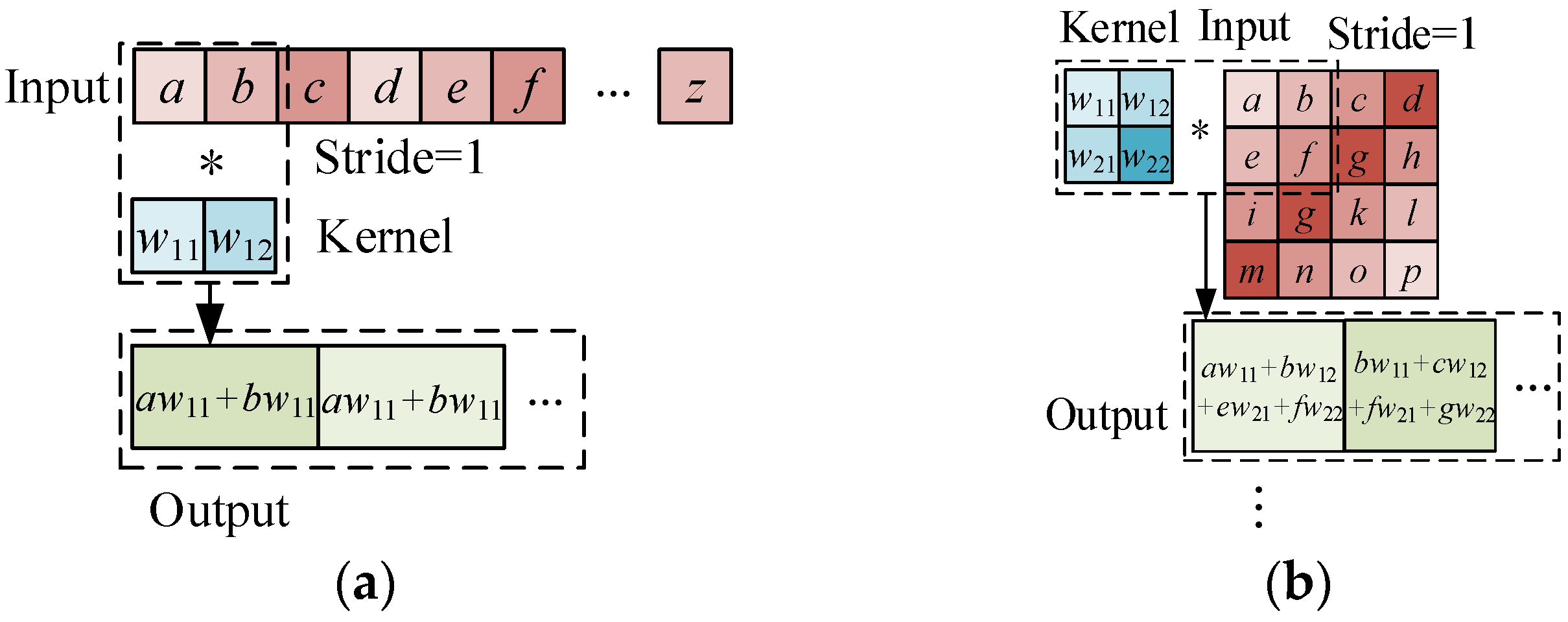
2.1. Convolutional Neural Network

Convolutional neural network (CNN) [37] is a typical deep learning model, which is mainly used to process grid data, such as voice, time series and images. Structural dynamic response data, as a type of time-series data, have been successfully predicted by using the CNN model in existing literature [24,27]. The basic concept is to use convolution operation, instead of fully connected layers, to extract features from the input data. This optimization realizes local connections and weight sharing which decrease the number of parameters. The definition of 1-D and 2-D convolutional operations in CNN can be expressed by Equations (1) and (2), respectively:

$$o_{i,k}=(x\ast v{)}_{i,k}={\displaystyle \sum _{l,m}{x}_{(i-1)s+m,l}{V}_{m,l,k}},$$

(1)

$$O_{i,j,k}=(X\ast V{)}_{i,j,k}={\displaystyle \sum _{l,m,n}{X}_{(i-1)s+m,(j-1)s+n,l}{V}_{m,n,l,k}},$$

(2)

where in Equation (1), x is the 1-D input, v is the convolutional kernel and o is the output. Similarly, in Equation (2), X is the input of the 2-D convolutional operation, and V and O are the corresponding kernel and output. The strides of convolutional operation, s, refers to how many data points are skipped between the two operations. The process of 1-D and 2-D convolution is expressed in Figure 1.

Pooling operation is another important operation used in CNN. The main function of pooling is to compress the data. There are mainly two types of pooling; mean pooling and maximum pooling. As its name implies, mean pooling outputs the mean value in the pooling region while maximum pooling outputs the maximum value.

A 1-D CNN model is used to predict the seismic response of the building. The architecture of the proposed CNN model is described in Figure 2. The input is the earthquake acceleration, while the output is the displacement or the acceleration response. There are five hidden convolutional layers and one fully connected layer between input and output layers. For the convolutional layer, rectified linear unit (ReLU) is used as the activation function.

2.2. Training of Bayesian Deep Learning Model

When the deep learning model is built, the model parameters, such as weight matrix and bias vector, can be estimated by using the samples of input and output. This process is the so-called ‘model training’. From the perspective of probability theory, when the point estimation is utilized, the trained deep learning model has deterministic values. However, if Bayesian estimation is applied, the probability distribution can be obtained. In Bayesian deep learning, the variational inference is used to realize the Bayesian estimation.

(1)

Variational inference

Let us consider a deep learning model with model parameter W. The set of training data includes M samples, such as: $S=\left\{\left(x_1,y_1\right),\left(x_2,y_2\right),\cdots ,\left(x_M,y_M\right)\right\}$. According to the Bayes formula [38], the model parameters are estimated as:

$$p\left(W|S\right)=\frac{p\left(S|W\right)p\left(W\right)}{p\left(S\right)}=\frac{p\left(S|W\right)p\left(W\right)}{{\displaystyle {\int }_{W}p\left(S|W\right)p\left(W\right)\mathrm{d}W}}$$

(3)

where p(W) is the prior distribution, which is determined by assumption, prior knowledge or experience. The distribution of train samples is p(S), p(S|W) is the likelihood function and p(W |S) is the estimated distribution of model parameter W. Since p(S) is difficult to obtain, the Bayes formula cannot be used to obtain the parameter estimation directly. To solve this problem, a new distribution q(W) is introduced to approximate p(θ|S). The difference between q(W) and p(W|S) can be measured through the concept of Kullback-Leibler (KL) divergence [39]. KL divergence can be expressed as:

$$\begin{array}{ll}{\mathrm{D}}_{\mathrm{KL}}\left(q(\theta )\left|\right|p(\theta |S)\right)& ={\displaystyle {\int }_{W}q(W)\log \frac{q(W)}{p(W|S)}}\mathrm{d}W\\ & ={\displaystyle {\int }_{\Theta }q(W)\log \frac{q(\theta ){\displaystyle {\int }_{W}p(S|W)p(W)dW}}{p(S|W)p(W)}}dW\\ & ={\displaystyle {\int }_{\Theta }q(W)p(S)}\mathrm{d}W-{\displaystyle {\int }_{\Theta }q(W)\log \frac{p(S|W)p(\theta )}{q(W)}}\mathrm{d}W\end{array}$$

(4)

The aim of variational inference is to obtain the optimal q(θ) by minimizing KL divergence, or, in essence, maximizing the second term in the left as:

$$q^{\ast }(W)=\underset{q(W)}{\arg \min }\mathrm{DKL}\left(q(W)\left|\right|p(W|S)\right)=\underset{q(W)}{\arg \max }{\displaystyle {\int }_{W}q(W)\log \frac{p(S|W)p(W)}{q(W)}}\mathrm{d}W,$$

(5)

In order to convert the variational problem to an optimization problem, the q(W) can be assumed to be a joint Gaussian distribution and every parameter W_i in the parameter matrix W obeys an independent Gaussian distribution as:

$$q(W)=N(W,\mu ,{\sigma }^2)={\displaystyle \prod _i^{n_{W_i}}N(W_i,{\mu }_i,{\sigma }_i^2)},$$

(6)

where μ and σ refer to the mean value matrix and the standard deviation. The optimal distribution q(W) can be obtained by finding the optimal value of parameter matrix μ and σ as:

$$\begin{array}{ll} {\mathsf{\mu }}^{\ast },{\mathsf{\sigma }}^{\ast }=& \underset{\mathbf{\mu },\mathbf{\sigma }}{\mathrm{argmax}}{\displaystyle \sum _{k=1}^{n_{\theta }}}{\mathbb{E}}_{q\left({\sigma }_k{\epsilon }_k+u_k\right)}\left[\log (p\left({\sigma }_k{\epsilon }_k+u_k\right))\right]\\ & +{\displaystyle \sum _{k=1}^{n_{\theta }}}{\mathbb{E}}_{q_k\left({\sigma }_k{\epsilon }_k+u_k\right)}\left[\log (q_k\left({\sigma }_k{\epsilon }_k+u_k\right))\right]\\ & +\frac{N_B}{N}{\displaystyle \sum _{j=1}^{N/N_B}}\frac{N}{N_B}{\displaystyle \sum _{i=1}^{N_B}}{\mathbb{E}}_{q\left(\epsilon \right)}\left[\log (p({\mathbf{y}}_i|{\mathbf{x}}_i,\mathsf{\mu },\mathsf{\sigma },\mathsf{\epsilon }))\right]\end{array}$$

(7)

(2)

Bayes back propagation algorithm

The Bayes back propagation algorithm [40,41] is used to train the proposed Bayesian deep learning model. This algorithm combines variational inference with the back propagation algorithm used in conventional deep learning model training. The object function in Equation (7) is used as an additional loss function L_KL to update the model parameters. The process of the Bayes back propagation algorithm can be expressed as follows:

Step 1: Initialize the mean and standard deviation value of random parameters as μ and σ.

Step 2: Select a batch of data from the training data.

Step 3: Generate random sample $\epsilon ~N(0,I)$ and calculate the random parameters as $W=\mu +\sigma \epsilon$.

Step 4: Calculate the total loss function as L_total = L_mse + L_KL, where L_mse is the mean square error function while L_KL is the KL divergence loss function as the object function in Equation (7).

Step 5: Calculate the $g_W^{\mathrm{mse}}$, $g_{\mu }^{\mathrm{KL}}$ and $g_{\sigma }^{\mathrm{KL}}$ which are the gradient to L_mse and L_KL by back propagation algorithm.

Step 6: Update the random parameter by gradient descent as:

$$\begin{gathered} \mu =\mu -\alpha \left(g_W^{\mathrm{mse}}+g_W^{\mathrm{KL}}+g_{\mu }^{\mathrm{KL}}\right), \\ \sigma =\sigma -\alpha \left(\left(g_W^{\mathrm{mse}}+g_W^{\mathrm{KL}}\right)\epsilon +g_{\sigma }^{\mathrm{KL}}\right) \end{gathered}$$

Step 7: Repeat steps 2 to 6 until the deep learning model is well trained.

Where α is the learning rate; some adaptive gradient descent, such as Adam or RMSprop [42], can also be applied to train the proposed Bayesian deep learning model to make the model convergence in less training epochs.

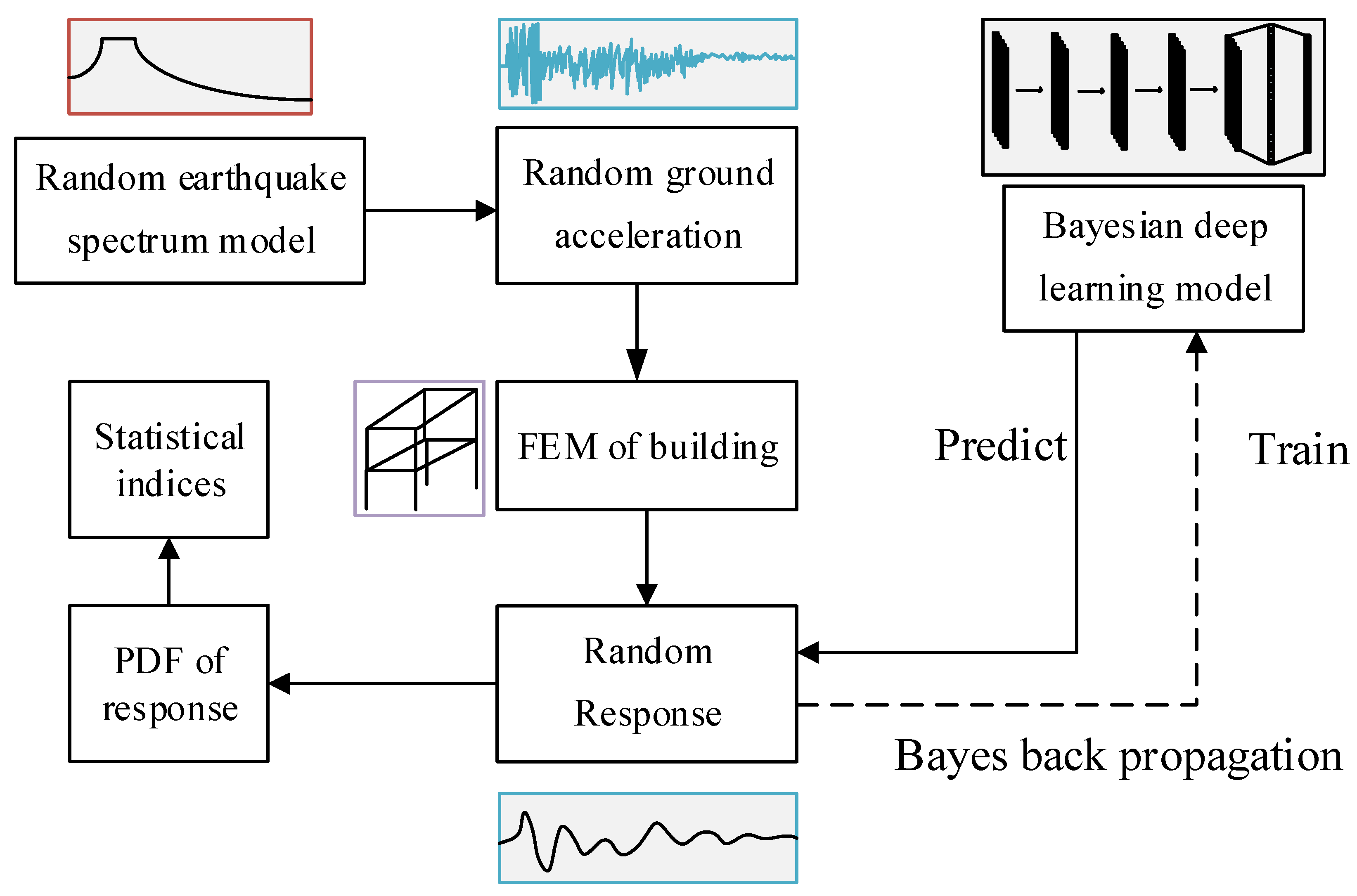
2.3. The Framework of Proposed Method

The framework of the proposed method is presented in Figure 3. A finite element model of a 3D building with random characteristics is built. Through Monte-Carlo simulation, samples of input ground motion acceleration and output structural response are generated. The training data are utilized to train the deep convolutional neural network through Bayes back propagation algorithm. The trained Bayesian deep learning model is used to predict the random response of the 3D building. The results are given in the form of probability distribution functions (PDFs) and the main statistical indices are expressed as mean value and standard deviation.

3. Three-Dimensional Random Building Structure

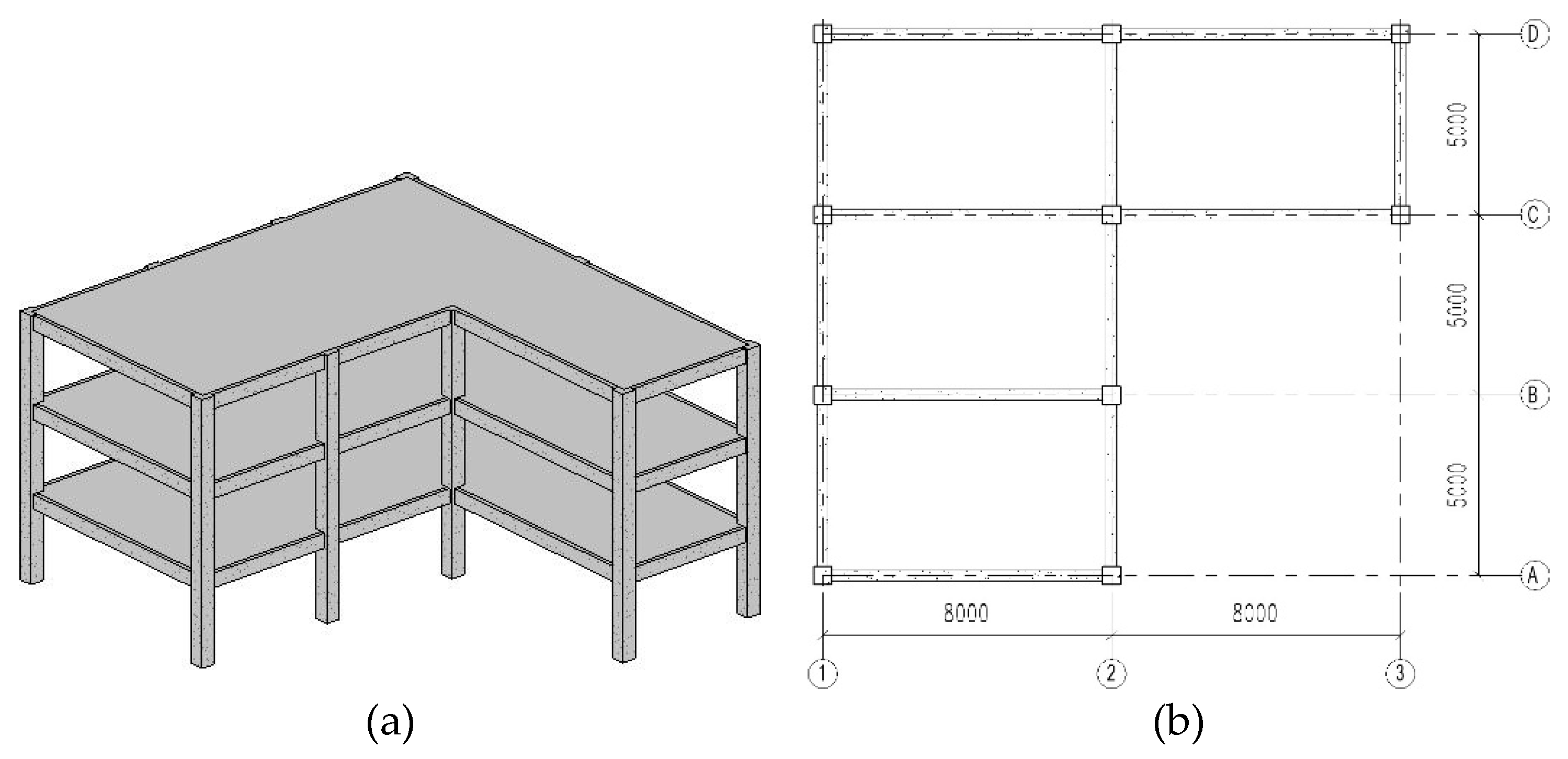
3.1. Three Dimensional Building with Random Characteristics

As shown in Figure 4, a three dimensional (3D) building structure with random parameters is utilized to validate the performance of the Bayesian deep learning model. For this building, the story height for each floor is 3.0 m. The section dimension of columns and beams are 500 mm × 500 mm and 500 mm × 300 mm, respectively. The slab thickness is equal to 20 cm. In addition to the self-weight of beams and slabs, a distributed dead load of 2.5 kN/m² and a live load with nominal value of 2.0 kN/m² are considered in the analysis. The material parameters of concrete and steel are considered as random parameters, as shown in

Table 1. The random parameter of single floor shearing structure.

Parameter	Mean Value	Variable Coefficient	Type of Distribution
Density of concrete (kg/m3)	2500	0.1	Gaussian distribution
Density of steel bar (kg/m3)	7600	0.1	Gaussian distribution
Elastic of concrete (GPa)	30.0	0.05	Gaussian distribution
Elastic of steel bar (GPa)	210	0.05	Gaussian distribution
Damping ratio	0.05	0.05	Gaussian distribution

.

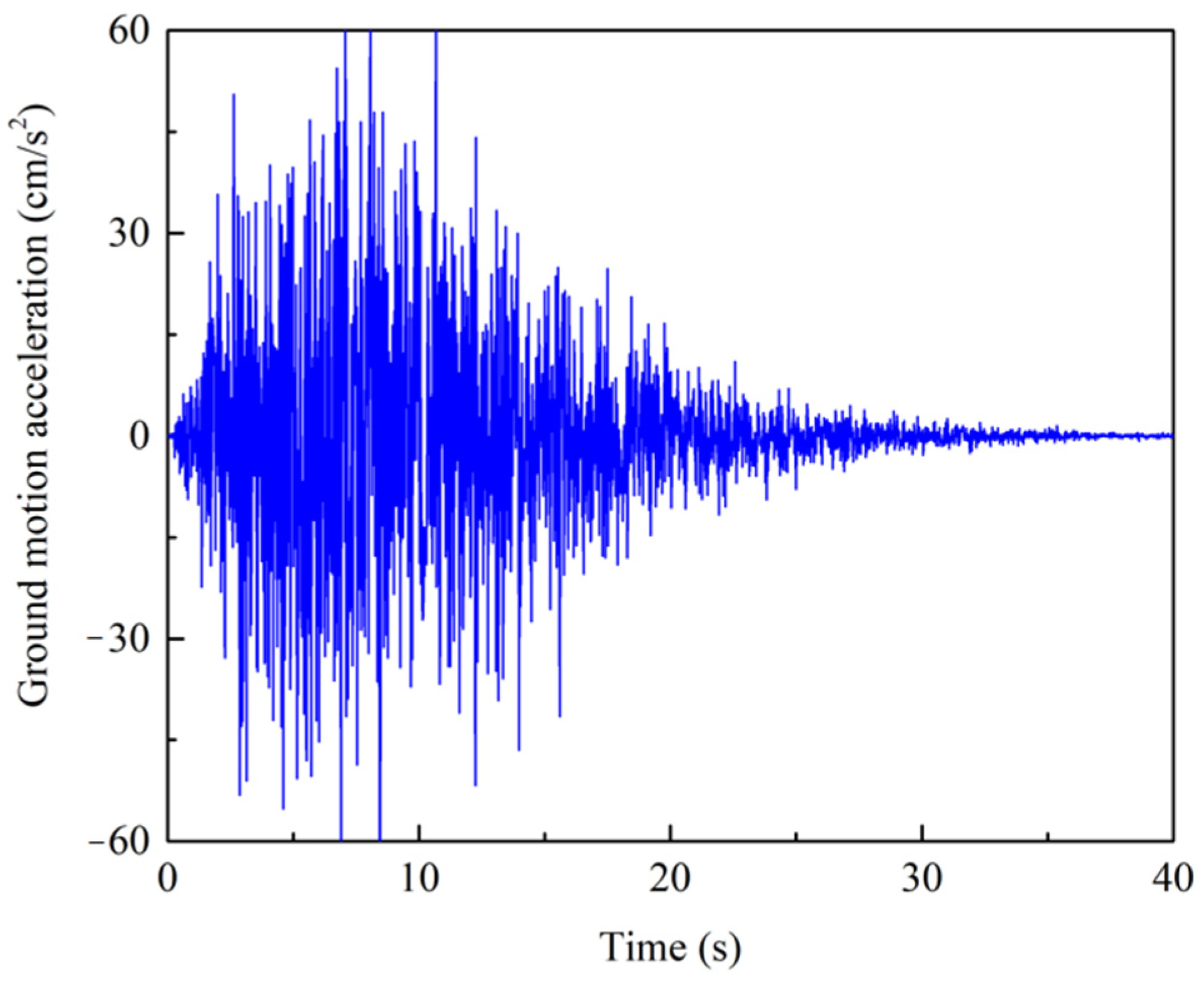
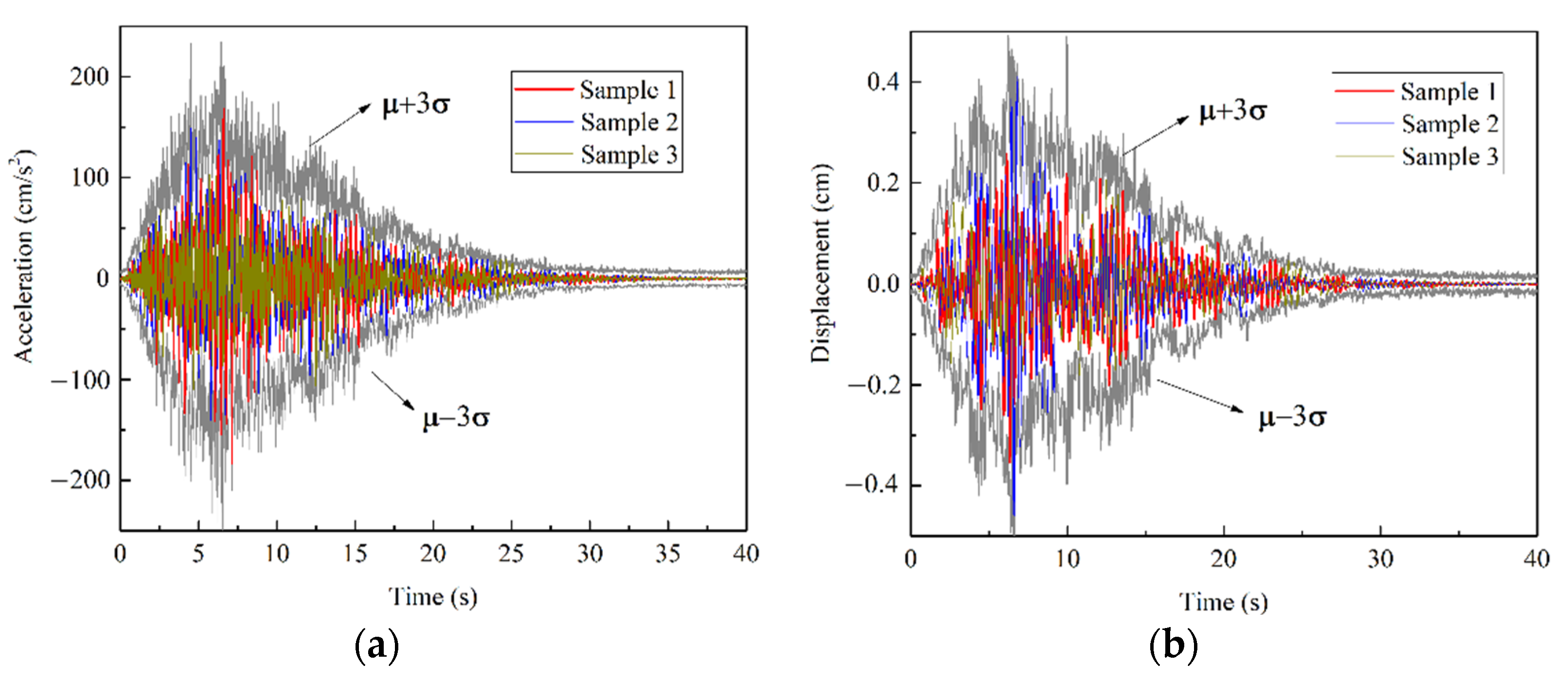
3.2. The Samples of Ground Motion Acceleration

In this paper, generalized the Kanai-Tajimi (GKT) [43,44,45] model is used to generate the samples of random ground motion acceleration. The GKT model can be expressed by Equations (8) and (9) as:

$${\ddot{X}}_{\mathrm{f}}\left(t\right)+2{\varsigma }_{\mathrm{g}}{\omega }_{\mathrm{g}}{\dot{X}}_{\mathrm{f}}\left(t\right)+{\omega }_{\mathrm{g}}^2{X}_{\mathrm{f}}\left(t\right)=\mathrm{wn}\left(t\right),$$

(8)

$${\ddot{X}}_{\mathrm{g}}\left(t\right)=-2\left({\varsigma }_{\mathrm{g}}{\omega }_{\mathrm{g}}{\dot{X}}_{\mathrm{f}}\left(t\right)+{\omega }_{\mathrm{g}}^2{X}_{\mathrm{f}}\left(t\right)\right)e\left(t\right),$$

(9)

where X_f(t) is the filtered response, ω_g is the characteristic ground frequency, ς_g is the effective ground damping coefficient, ${\ddot{X}}_{\mathrm{g}}(t)$ is the output ground acceleration, e(t) is the amplitude envelope function, and wn(t) is a stationary white noise process. In this paper, the amplitude envelope function can be written as:

$$E\left(t\right)=a{\left(\frac{t}{t_n}\right)}^b\exp (-c\frac{t}{t_n}),$$

(10)

$$b=-\frac{{\epsilon }_t\ln \eta }{1+{\epsilon }_t\left(\ln \eta -1\right)},c=-\frac{b}{{\epsilon }_t},a={\left(\frac{\exp (1)}{{\epsilon }_t}\right)}^b,$$

(11)

where t_n is the duration time of the earthquake, ${\epsilon }_t$ is normalized time when ground motion peak appears, and $\eta$ is the value of ground motion at 90% of the duration time.

The 3D building is considered to be located in a 2nd class site and the design earthquake group belongs to group 2. According to the Chinese code for seismic design of buildings and related literature [46,47], the parameters ${\omega }_{\mathrm{g}}$ and ${\varsigma }_{\mathrm{g}}$ are selected as ω_g = 15.7 rad/s and ς_g = 0.72. A frequent earthquake with intensity of VII is considered. Therefore, the spectral intensity of the stationary white noise process S₀ is equal to 15.21 cm²/s³. The parameters of amplitude envelope function are given as: $\eta =0.1$, ${\epsilon }_t=0.2$ and t_n = 40 s. Figure 5 presents a sample generated by the GKT model.

3.3. Modeling and Dynamic Response Analysis of 3D Building

The 3D building is modeled by OpenSees [46] for further analysis. The analytic model in OpenSees can be described as in Figure 6. Every column and beam in the building is modeled through fiber approach [47]. Each fiber in the column or beam section can be assigned as a concrete or steel bar in order to simulate their combined action. The earthquake wave is applied in the direction of North to South (NS). The displacement and acceleration response of point A to C (as shown in Figure 6) is presented in Figure 7.

4. Numerical Results

4.1. Model Training

To validate the random response prediction capacity of the proposed Bayesian deep learning model, 1000 samples were generated by 3D building FE model through Monte-Carlo simulation. Out of these samples, 500 were utilized for model training while the rest were used for validation and analysis. Bayes back propagation algorithm and RMSprop algorithm were used to train the proposed Bayesian deep learning model and the initial learning rate was equal to 0.0001. The training process is presented in Figure 8 which describes the loss function, varied with training epochs. As shown, the total losses of Bayesian deep learning were reduced during modeling and after 80 epochs; the total losses arrived at the level of 10⁻⁴. This means the proposed model can be well trained by using the back propagation algorithm.

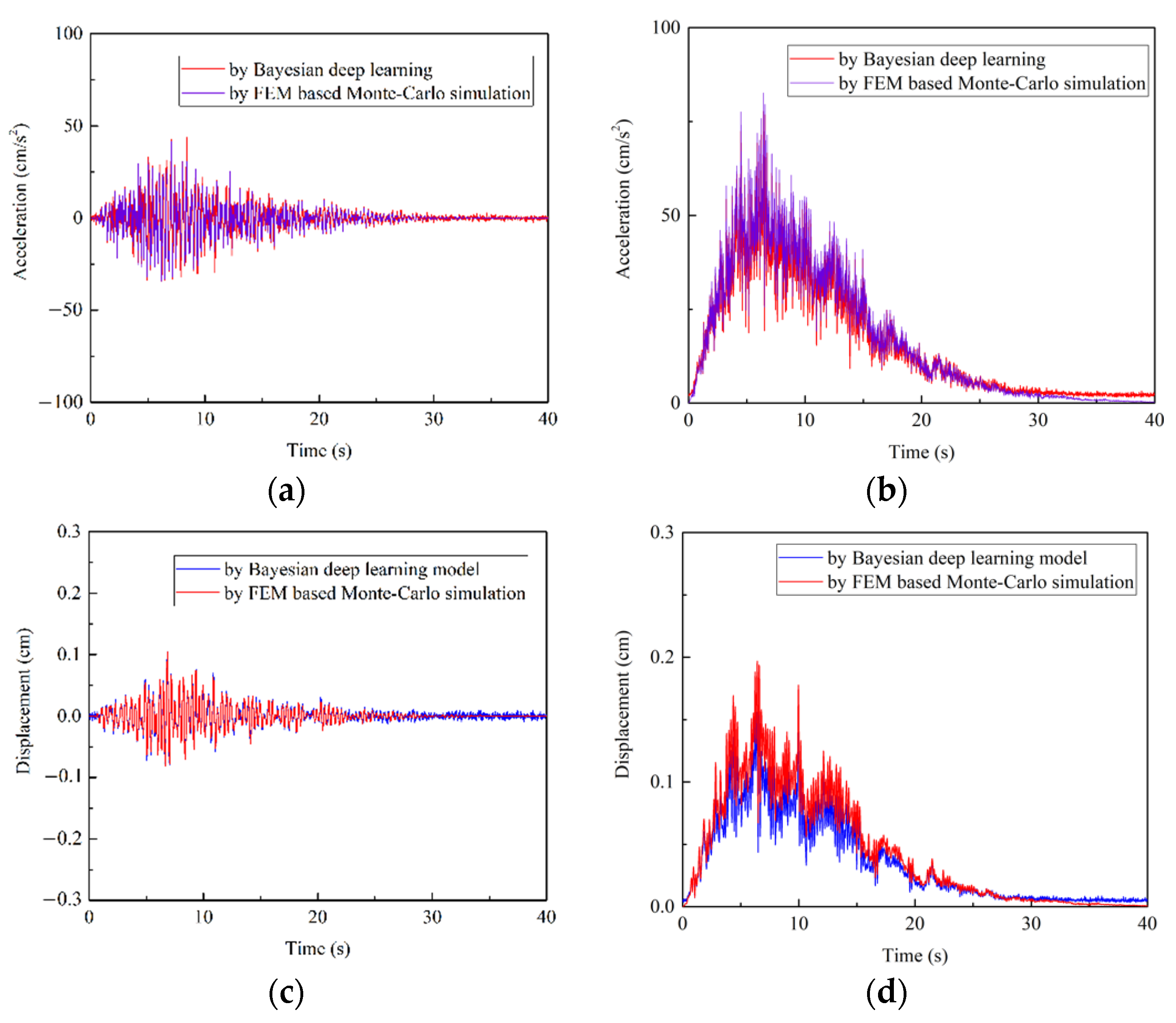
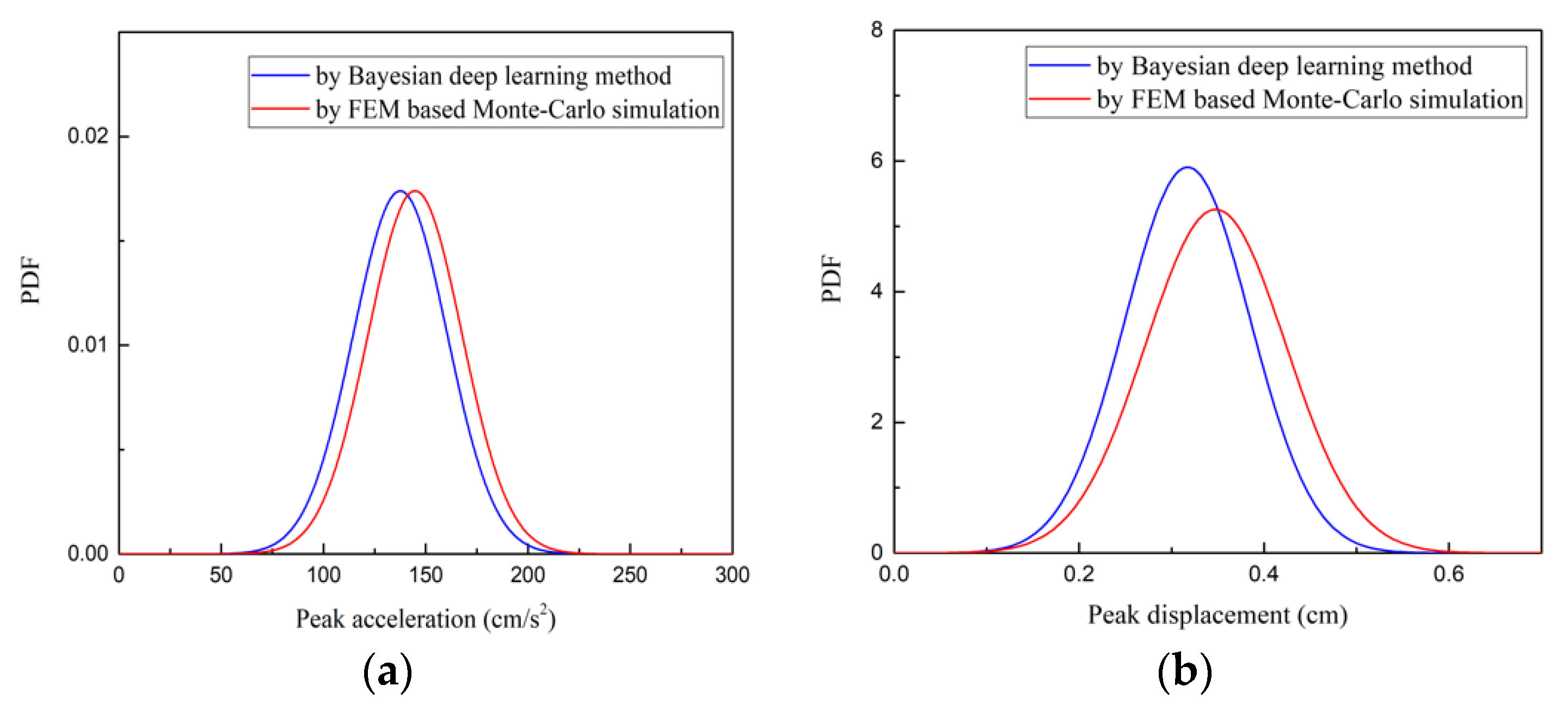
4.2. Response Prediction Results

The response prediction results are provided in the form of PDF, illustrated in Figure 9. Since the shapes of time history response curvatures at A, B and C points were similar, we only discuss the response at point A as our example. As shown in Figure 10, the samples of random response can be included in the section of [μ − 3σ, μ + 3σ], where μ is the mean value of response and σ is the standard deviation at point A. This result coincides with the conclusion of Gaussian distribution in probability theory. Figure 11 further compares the difference between Bayesian deep learning prediction results and Monte-Carlo simulation results in the mean value and standard deviation. The PDF of prediction result was close to the PDF from FEM based Monte-Carlo simulation. The normalized mean square errors (MSEs) of mean value were 1.92 × 10⁻⁵ (acceleration) and 5.05 × 10⁻⁵ (displacement), while the normalized MSEs of standard deviation were 1.17 × 10⁻⁴ (acceleration) and 5.10 × 10⁻⁴ (displacement). The peak errors of mean value were 2.56% and 5.99%, while the standard deviations were 5.34% and 10.23%. It was found that the prediction results of acceleration response had higher accuracy. This might be due to the weaker correlation between ground motion acceleration and structural displacement response.

Figure 12 presents, and compares, the PDFs of peak value of acceleration and displacement responses at point A. The proposed Bayesian deep learning method can provide an effective probabilistic estimation of the peak response. The proposed method can be used as a surrogate model for seismic reliability analysis when it is combined with Monte-Carlo simulation and first passage probability theory.

5. Discussion

In this section, the influence of structural parameter randomness and the input noise level are discussed. The PDF of peak acceleration and peak displacement are compared, as well as their mean value and standard deviation value. Furthermore, two indices, below, are introduced as:

$$Erro{r}_{\mathrm{mean}}=\frac{\left|\mathrm{Mean}\left(\mathrm{Peak}\left(X\left(t\right)\right)\right)-\mathrm{Mean}\left(\mathrm{Peak}\left(\widehat{X}\left(t\right)\right)\right)\right|}{\left|\mathrm{Mean}\left(\mathrm{Peak}\left(X\left(t\right)\right)\right)\right|}$$

(12)

$$Erro{r}_{\mathrm{stdv}}=\frac{\left|\mathrm{Std}(\mathrm{Peak}(X(t)))-\mathrm{Std}(\mathrm{Peak}(\widehat{X}(t)))\right|}{\left|\mathrm{Std}(\mathrm{Peak}(X(t)))\right|},$$

(13)

where $X(t)$ is the building response at point A, calculated by FEM, and $\widehat{X}(t)$ is the prediction response. Peak ( ) is the peak value function, which selects the absolute maximum value from input. Mean ( ) is used to calculate the mean value of the input and Std ( ) calculates the standard deviation of the input. Equations (12) and (13) present the prediction errors of mean value and standard deviation value.

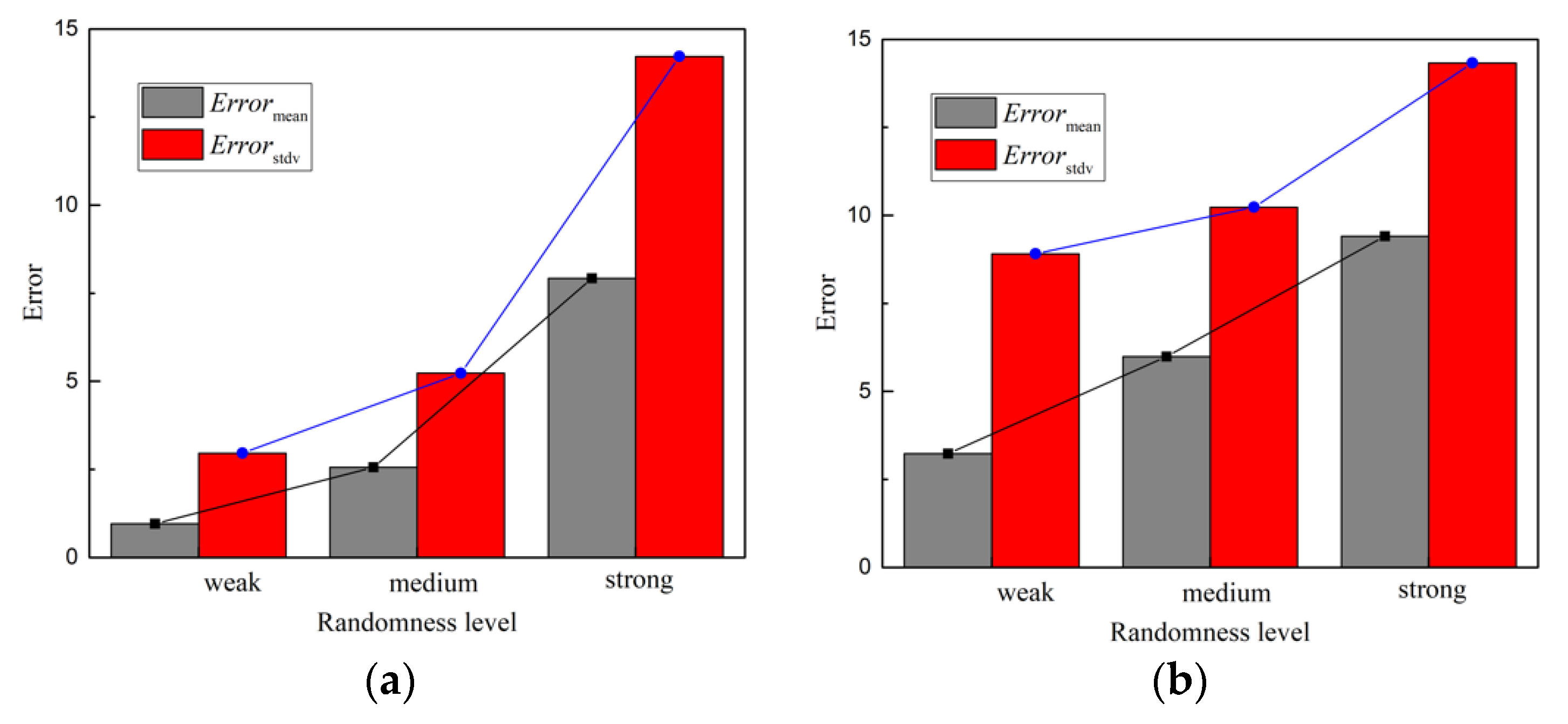
5.1. Influence of Parameter Randomness

To discuss the influence of parameter randomness, we considered three different levels of randomness. The variable coefficients of all random parameters were 0.5, 1 and 2 times the original coefficients, respectively. Slight randomness corresponds to 0.5 times variable coefficients, while 1.0 and 2.0 times correspond to medium and strong randomness. Figure 13 presents and compares the Error_mean and Error_stdv of acceleration and displacement responses at point A under different randomness levels. It can be concluded that, as the randomness of the structure parameters increases, the prediction errors increase. Due to the uncertainty simulation capacity of Bayesian deep learning, the increases in errors are considered to be limited.

5.2. Influence of Input Noise

Robustness is the anti-noise capacity of the proposed model. In engineering practice, the input ground motion acceleration signal is polluted by noise from different sources. Therefore, robustness is very important to a deep learning model for response prediction. To discuss the influence of noise in input ground motion and the robustness of the deep learning model, ground motion data were added with 1%, 2%, 5%, 10% and 20% Gaussian white noise [48]. Figure 14 shows the Error_mean and Error_std of acceleration and displacement prediction results at point A. The mean value prediction result remained stable under different noise levels but the standard deviation results fluctuated with the noise level. However, there was no evidence that noise would influence the standard deviation prediction results, since Error_std does not increase with noise level. Therefore, the proposed Bayesian deep learning model is robust, even in the case of a high noise level. This is an advantage of the proposed model.

6. Conclusions

In this paper, a Bayesian deep learning method was proposed to predict the seismic response of a structure with random characteristics. A deep convolutional neural network, with random parameters, was established to predict the structural response. Bayes back propagation algorithm was introduced to train the deep learning model. To validate the proposed model, a 3D building structure model with random parameters was constructed in OpenSees to obtain the random response under a GKT earthquake. The Bayesian deep learning model was utilized to predict the PDF of the response. The influence of randomness of structural parameters and the noise due to ground motion were discussed. The following conclusions can be drawn:

(1)

The proposed Bayesian deep learning model can reliably predict the random response of a 3D building structure with random parameters and obtain the PDF of response. The prediction of mean value is better than the prediction of standard deviation because of the parameter randomness.

(2)

As the parameter randomness increases, the effective performance of Bayesian deep learning model deteriorates. Compared with mean value prediction, the standard deviation prediction is more seriously affected by parameter randomness.

(3)

Input noises have very little influence on the proposed Bayesian deep learning model. The proposed model is robust and can work under a high noise level of 20%. Therefore, the proposed model has promising potential for practical applications in civil, mechanical, and aerospace engineering.

References

1. Aslani, H.; Miranda, E. Probability-based seismic response analysis. Eng. Struct. 2005, 27, 1151–1163. [Google Scholar] [CrossRef]
2. Chopra, A.K. Dynamics of Structures; Pearson Education, Prentice Hall: Hoboken, NJ, USA, 2011. [Google Scholar]
3. Ibrahim, R.A. Structural Dynamics with Parameter Uncertainties. ASME Appl. Mech. Rev. March 1987, 40, 309–328. [Google Scholar] [CrossRef]
4. Desceliers, C.; Soize, C.; Cambier, S. Non-parametric–parametric model for random uncertainties in non-linear structural dynamics: Application to earthquake engineering. Earthq. Eng. Struct. Dyn. 2004, 33, 315–327. [Google Scholar] [CrossRef] [Green Version]
5. Silik, A.; Noori, M.; Altabey, W.A.; Ghiasi, R. Selecting optimum levels of wavelet multi-resolution analysis for time-varying signals in structural health monitoring. Struct. Control Health Monit. 2021, 28, e2762. [Google Scholar] [CrossRef]
6. Silik, A.; Noori, M.; Altabey, W.A.; Ghiasi, R.; Wu, Z. Comparative Analysis of Wavelet Transform for Time-Frequency Analysis and Transient Localization in Structural Health Monitoring. Struct. Durab. Health Monit. 2021, 15, 1–22. [Google Scholar] [CrossRef]
7. Silik, A.; Noori, M.; Altabey, W.; Dang, J.; Ghiasi, R.; Wu, Z. Optimum wavelet selection for nonparametric analysis toward structural health monitoring for processing big data from sensor network: A comparative study. Struct. Health Monit. 2021, 21, 803–825. [Google Scholar] [CrossRef]
8. Silik, A.; Noori, M.; Altabey, W.; Ghiasi, R.; Wu, Z. Analytic Wavelet Selection for Time–Frequency Analysis of Big Data Form Civil Structure Monitoring. Lect. Notes Civ. Eng. 2021, 156, 431–455. [Google Scholar] [CrossRef]
9. Pradlwarter, H.J.; Schuëller, G.I. On advanced Monte Carlo simulation procedures in stochastic structural dynamics. Int. J. Non-Linear Mech. 1997, 32, 735–744. [Google Scholar] [CrossRef]
10. Ibarra, L.; Krawinkler, H. Variance of collapse capacity of SDOF systems under earthquake excitations. Earthq. Eng. Struct. Dyn. 2011, 40, 1299–1314. [Google Scholar] [CrossRef]
11. Liao, S.; Li, J. A stochastic approach to site-response component in seismic ground motion coherency model. Soil Dyn. Earthq. Eng. 2002, 22, 813–820. [Google Scholar] [CrossRef]
12. Li, J.; Chen, J.; Sun, W.; Peng, Y. Advances of the probability density evolution method for nonlinear stochastic systems. Probabilistic Eng. Mech. 2012, 28, 132–142. [Google Scholar] [CrossRef]
13. Huang, Y.; Xiong, M.; Zhou, H. Ground seismic response analysis based on the probability density evolution method. Eng. Geol. 2015, 198, 30–39. [Google Scholar] [CrossRef]
14. Liu, Z.; Liu, Z.; Xu, Y. Probability density evolution analysis of a shear-wall structure under stochastic ground motions by shaking table test. Soil Dyn. Earthq. Eng. 2019, 122, 53–66. [Google Scholar]
15. Liu, Z.; Ruan, X.; Liu, Z.; Lu, H. Probability density evolution analysis of stochastic nonlinear structure under non-stationary ground motions. Struct. Infrastruct. Eng. 2019, 15, 1049–1059. [Google Scholar] [CrossRef]
16. LeCun, Y.; Bengio, Y.; Hinton, G. Deep learning. Nature 2015, 521, 436–444. [Google Scholar] [CrossRef]
17. Ghaboussi, J.; Joghataie, A. Active control of structures using neural networks. J. Eng. Mech. 1995, 121, 555–567. [Google Scholar] [CrossRef]
18. Chen, H.M.; Qi, G.Z.; Yang, J.C.S.; Amini, F. Neural network for structural dynamic model identification. J. Eng. Mech. 1995, 121, 1377–1381. [Google Scholar] [CrossRef]
19. Pei, J.S.; Smyth, A.W.; Kosmatopoulos, E.B. Analysis and modification of Volterra/Wiener neural networks for the adaptive identification of non-linear hysteretic dynamic systems. J. Sound Vib. 2004, 275, 693–718. [Google Scholar] [CrossRef]
20. Lagaros, N.D.; Papadrakakis, M. Neural network based prediction schemes of the non-linear seismic response of 3D buildings. Adv. Eng. Softw. 2012, 44, 92–115. [Google Scholar] [CrossRef]
21. Joghataie, A.; Farrokh, M. Dynamic analysis of nonlinear frames by Prandtl neural networks. J. Eng. Mech. 2008, 134, 961–969. [Google Scholar] [CrossRef]
22. Xie, S.L.; Zhang, Y.H.; Chen, C.H.; Zhang, X.N. Identification of nonlinear hysteretic systems by artificial neural network. Mech. Syst. Signal Process. 2013, 34, 76–87. [Google Scholar] [CrossRef]
23. Farrokh, M.; Dizaji, M.S.; Joghataie, A. Modeling hysteretic deteriorating behavior using generalized Prandtl neural network. J. Eng. Mech. 2015, 141, 04015024. [Google Scholar] [CrossRef]
24. Wu, R.T.; Jahanshahi, M.R. Deep convolutional neural network for structural dynamic response estimation and system identification. J. Eng. Mech. 2019, 145, 04018125. [Google Scholar] [CrossRef]
25. Kim, T.; Kwon, O.S.; Song, J. Response prediction of nonlinear hysteretic systems by deep neural networks. Neural Netw. 2019, 111, 1–10. [Google Scholar] [CrossRef]
26. Zhang, R.; Liu, Y.; Sun, H. Physics-guided convolutional neural network (PhyCNN) for data-driven seismic response modeling. Eng. Struct. 2020, 215, 110704. [Google Scholar] [CrossRef]
27. Zhang, R.; Chen, Z.; Chen, S.; Zheng, J.; Büyüköztürk, O.; Sun, H. Deep long short-term memory networks for nonlinear structural seismic response prediction. Comput. Struct. 2019, 220, 55–68. [Google Scholar] [CrossRef]
28. Wang, C.; Xu, L.Y.; Fan, J.S. A general deep learning framework for history-dependent response prediction based on UA-Seq2Seq model. Comput. Methods Appl. Mech. Eng. 2020, 372, 113357. [Google Scholar] [CrossRef]
29. Eshkevari, S.S.; Takáč, M.; Pakzad, S.N.; Jahani, M. DynNet: Physics-based neural architecture design for nonlinear structural response modeling and prediction. Eng. Struct. 2021, 229, 111582. [Google Scholar] [CrossRef]
30. Peng, H.; Yan, J.; Yu, Y.; Luo, Y. Structural Surrogate Model and Dynamic Response Prediction with Consideration of Temporal and Spatial Evolution: An Encoder–Decoder ConvLSTM Network. Int. J. Struct. Stab. Dyn. 2021, 21, 2150140. [Google Scholar] [CrossRef]
31. Wang, H.; Wu, T. Knowledge-enhanced deep learning for wind-induced nonlinear structural dynamic analysis. J. Struct. Eng. 2020, 146, 04020235. [Google Scholar] [CrossRef]
32. Li, H.; Wang, T.; Wu, G. Dynamic response prediction of vehicle-bridge interaction system using feedforward neural network and deep long short-term memory network. Structures 2021, 34, 2415–2431. [Google Scholar] [CrossRef]
33. Kim, T.; Song, J.; Kwon, O.S. Probabilistic evaluation of seismic responses using deep learning method. Struct. Saf. 2020, 84, 101913. [Google Scholar] [CrossRef]
34. Li, H.; Wang, T.; Wu, G. A Bayesian deep learning approach for random vibration analysis of bridges subjected to vehicle dynamic interaction. Mech. Syst. Signal Process. 2022, 170, 108799. [Google Scholar] [CrossRef]
35. Wang, T.; Li, H.; Noori, M. Response Prediction of Random Structure Based on Bayesian Neural Network. In Lecture Notes in Civil Engineering, Proceedings of the 7th International Conference on Architecture, Materials and Construction, Lisbon, Portugal, 27–29 October 2021; Springer-Nature: Berlin, Germany, 2021; pp. 19–25. ISBN 978-3-030-94513-8. [Google Scholar]
36. Wang, H.; Yeung, D.Y. A survey on Bayesian deep learning. ACM Comput. Surv. CSUR 2020, 53, 1–37. [Google Scholar] [CrossRef]
37. Albawi, S.; Mohammed, T.A.; Al-Zawi, S. Understanding of a convolutional neural network. In Proceedings of the 2017 International Conference on Engineering and Technology (ICET), Antalya, Turkey, 21–23 August 2017; pp. 1–6. [Google Scholar]
38. Yuen, K.V. Bayesian Methods for Structural Dynamics and Civil Engineering; John Wiley & Sons: Hoboken, NJ, USA, 2010. [Google Scholar]
39. Hershey, J.R.; Olsen, P.A. Approximating the Kullback Leibler divergence between Gaussian mixture models. In Proceedings of the 2007 IEEE International Conference on Acoustics, Speech and Signal Processing, Honolulu, HI, USA, 15–20 April 2007; Volume 4, pp. 4–317. [Google Scholar]
40. Graves, A. Practical variational inference for neural networks. In Proceedings of the 24th International Conference on Neural Information Processing Systems, Granada, Spain, 12–15 December 2011; pp. 2348–2356. [Google Scholar]
41. Blundell, C.; Cornebise, J.; Kavukcuoglu, K.; Wierstra, D. Weight uncertainty in neural network. In Proceedings of the 32nd International Conference on Machine Learning, Lille, France, 6–11 July 2015; pp. 1613–1622. [Google Scholar]
42. Goodfellow, I.; Bengio, Y.; Courville, A. Deep Learning; MIT Press: Cambridge, MA, USA, 2016. [Google Scholar]
43. Lin, Y.K.; Yong, Y. Evolutionary kanai-tajimi earthquake models. J. Eng. Mech. 1987, 113, 1119–1137. [Google Scholar] [CrossRef]
44. Rofooei, F.R.; Mobarake, A.; Ahmadi, G. Generation of artificial earthquake records with a nonstationary Kanai–Tajimi model. Eng. Struct. 2001, 23, 827–837. [Google Scholar] [CrossRef]
45. Guo, Y.; Kareem, A. System identification through nonstationary data using time–frequency blind source separation. J. Sound Vib. 2016, 371, 110–131. [Google Scholar] [CrossRef]
46. Ministry of Housing and Urban-Rural Development of the People’s Republic of China. Code for Seismic Design of Building GB50011-2010 (2016 Edition); China Architecture and Building Press: Beijing, China, 2016. (In Chinese) [Google Scholar]
47. Bai, G.; Zhu, L. Study on the parameters of Kanai-Tajimi model based on the code (GB50011-2001). World Earthq. Eng. 2004, 20, 114–118. (In Chinese) [Google Scholar]
48. Zhu, X.Q.; Law, S. Orthogonal function in moving loads identification on a multi-span bridge. J. Sound Vib. 2001, 245, 329–345. [Google Scholar] [CrossRef]
Figure 1. 1-D and 2-D convolution operation: (a) 1-D convolution; (b) 2-D convolution.
Sensors 22 03775 g001
Figure 2. The architecture of the proposed CNN model for response prediction.
Sensors 22 03775 g002
Figure 3. The framework of proposed method.
Sensors 22 03775 g003
Figure 4. The diagram of 3D building: (a) 3D view; (b) plane view (Unit: mm).
Sensors 22 03775 g004
Figure 5. The sample of ground motion acceleration of GKT model.
Sensors 22 03775 g005
Figure 6. The finite element model of 3D building: (a) Analytic model; (b) Fiber approach.
Sensors 22 03775 g006
Figure 7. The response of 3D building under GKT ground motion: (a) acceleration; (b) displacement.
Sensors 22 03775 g007aSensors 22 03775 g007b
Figure 8. The total loss of Bayesian deep learning model varies with training epochs.
Sensors 22 03775 g008
Figure 9. The PDF of response prediction result: (a) acceleration response; (b) displacement response. First row: point A response; Second row: point B response; point C response.
Sensors 22 03775 g009aSensors 22 03775 g009b
Figure 10. The comparison of Bayesian deep learning prediction results and results from FEM based Monte-Carlo simulation at point A: (a) acceleration; (b) displacement.
Sensors 22 03775 g010
Figure 11. The comparison of statistical indices at point A: (a) acceleration mean value; (b) acceleration standard deviation; (c) displacement mean value; (d) displacement standard deviation.
Sensors 22 03775 g011
Figure 12. The comparison of PDF of peak value at point A: (a) peak acceleration; (b) peak displacement.
Sensors 22 03775 g012
Figure 13. The comparison of peak error under different randomness level: (a) acceleration response; (b) displacement response.
Sensors 22 03775 g013
Figure 14. The comparison of peak errors under different noise levels: (a) acceleration response; (b) displacement response.
Sensors 22 03775 g014