
Acoustic Denoising Using Artificial Intelligence for Wood-Boring Pests Semanotus bifasciatus Larvae Early Monitoring

 ,
,
Abstract
:1. Introduction
- (1)
- The piezoelectric sensor connected with a voltage collection module was used to record the feeding sounds of Semanotus bifasciatus larvae.
- (2)
- The time domain denoising models based on the standard convolutions and dilated convolutions were designed to denoise the noisy feeding sounds according to the waveforms.
- (3)
- The frequency domain denoising models based on different recurrent layers were designed to denoise the noisy feeding sounds according to the spectrograms.
- (4)
- The denoising effects of different denoising models were evaluated and compared from the perspective of waveform and spectrum.
2. Data Materials
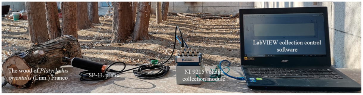
2.1. Data Recording
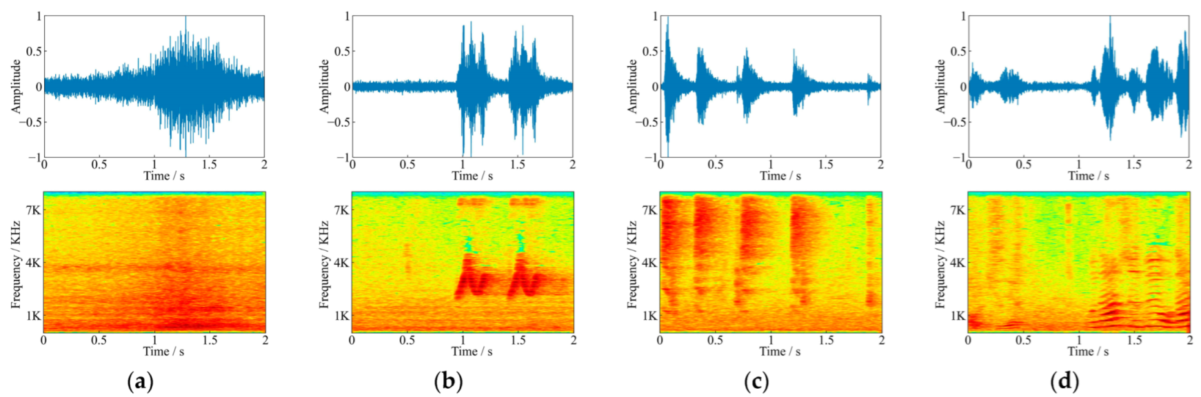
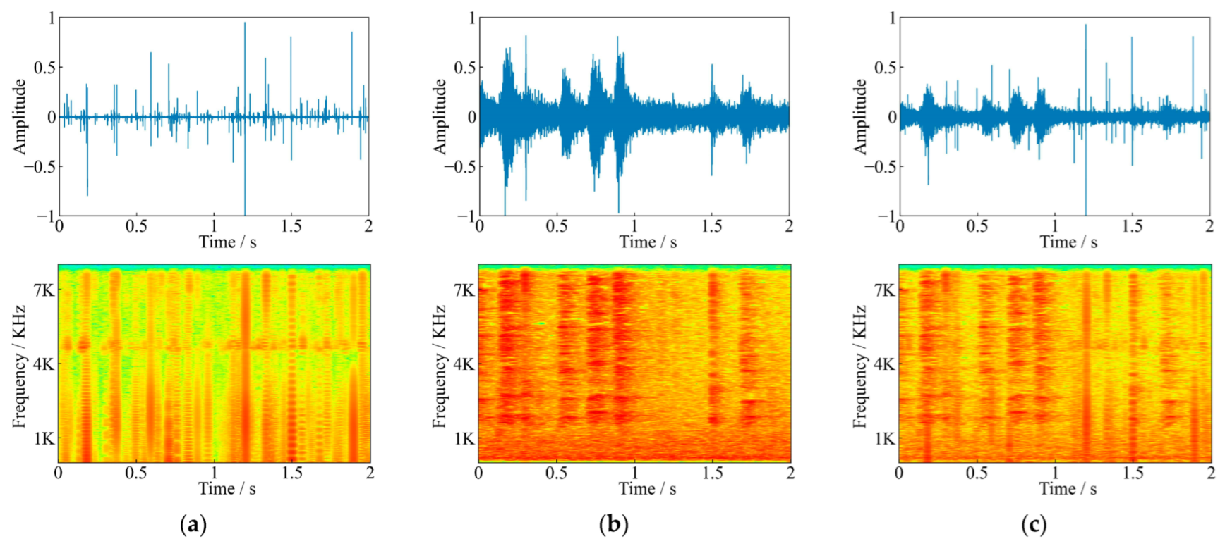
2.2. Dataset Construction
3. Denoising Models Based on Artificial Intelligence
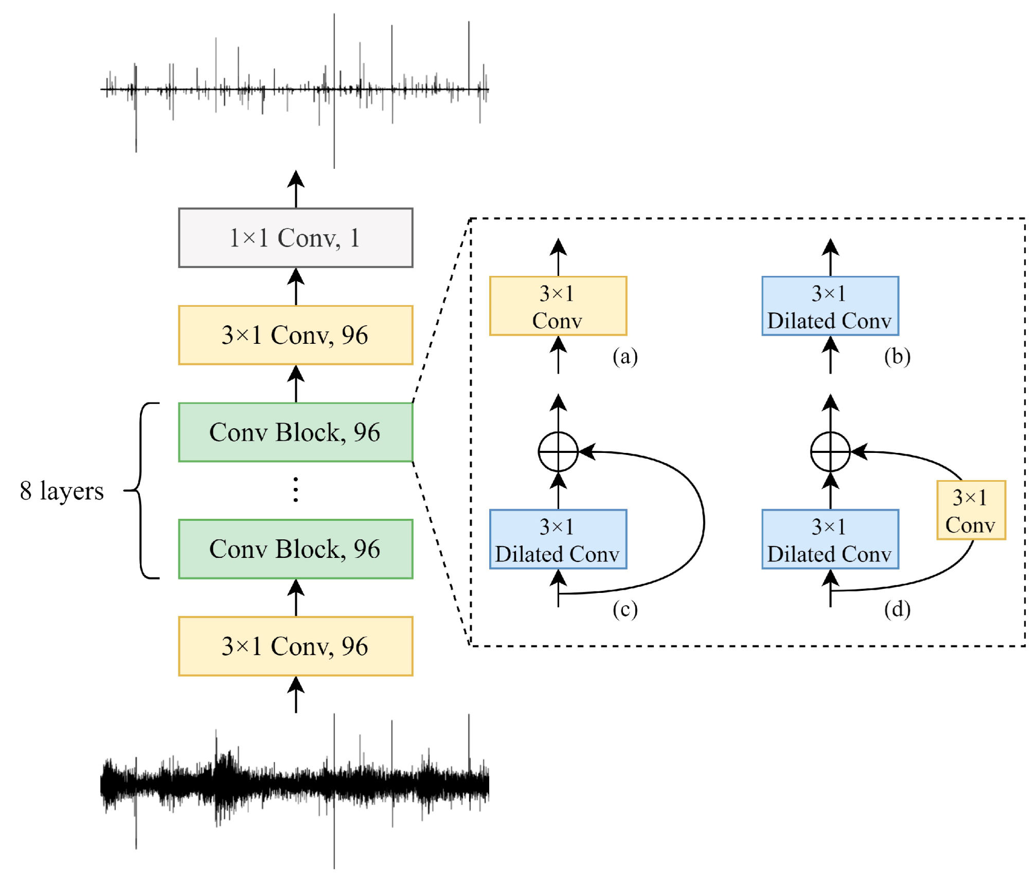
3.1. Time Domain Denoising Networks
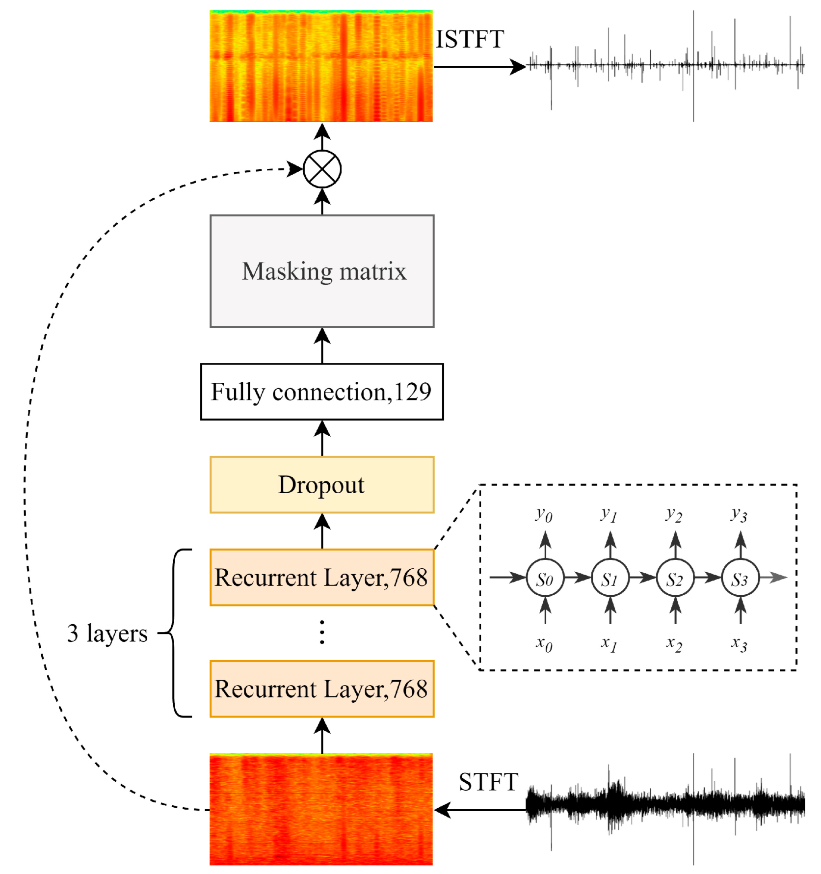
3.2. Frequency Domain Denoising Networks
4. Experiments and Results
4.1. Implementation Details
4.2. Evaluation Metrics for Denoising
4.3. Respective Results of TDD-Nets and FDD-Nets
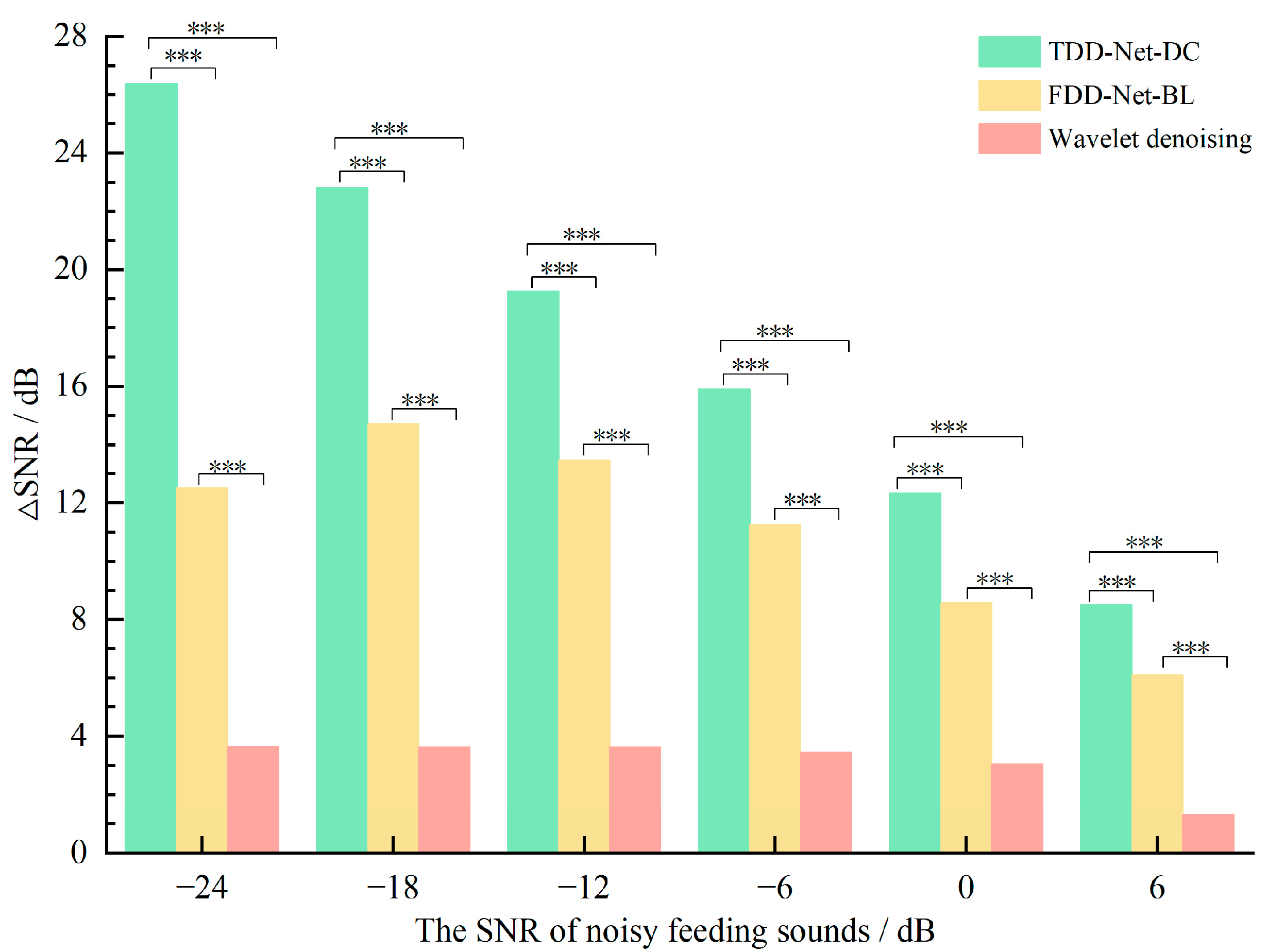
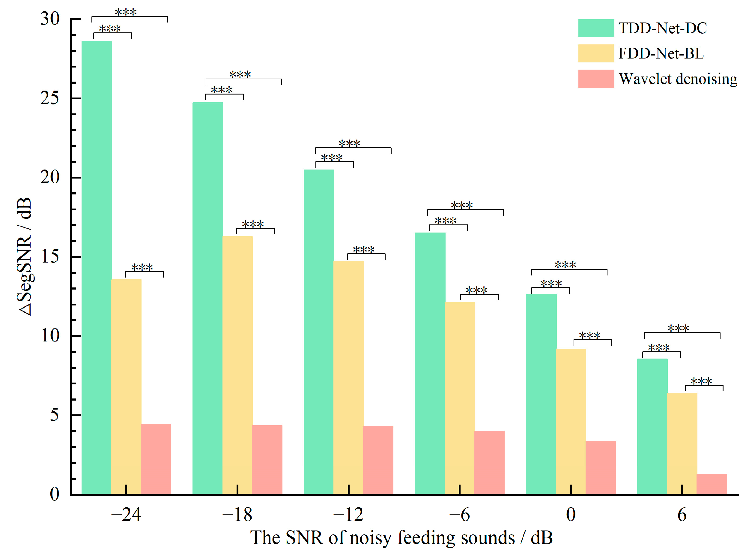
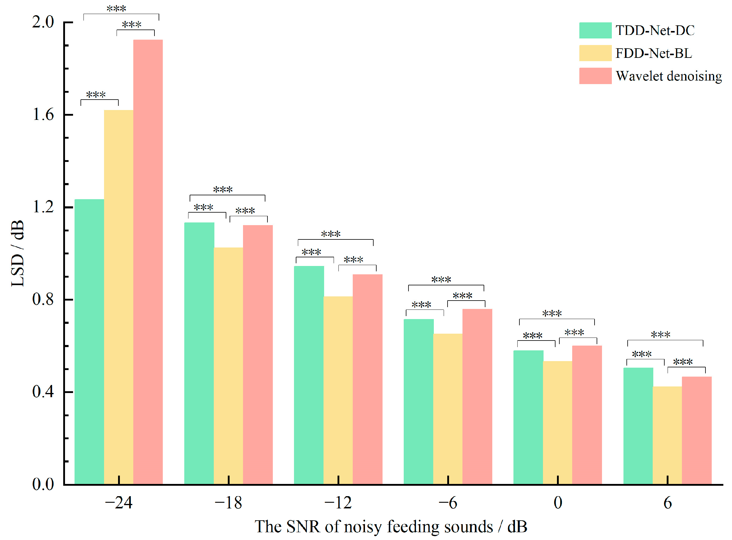
4.4. Comparisons between the Best TDD-Nets and FDD-Nets
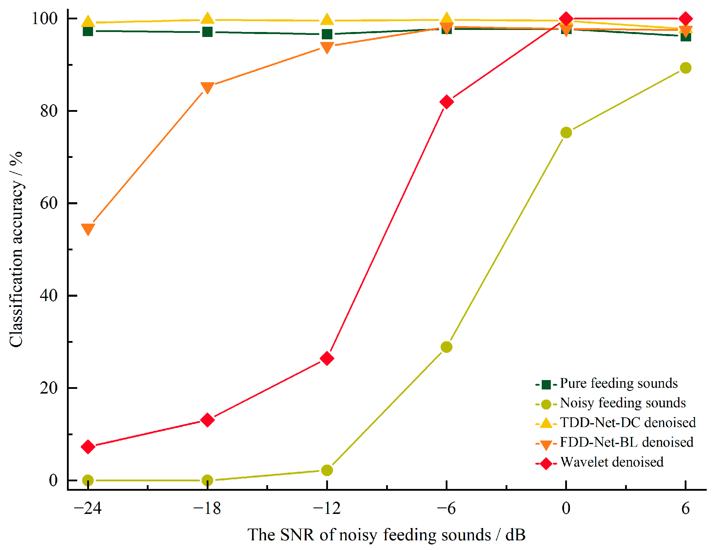
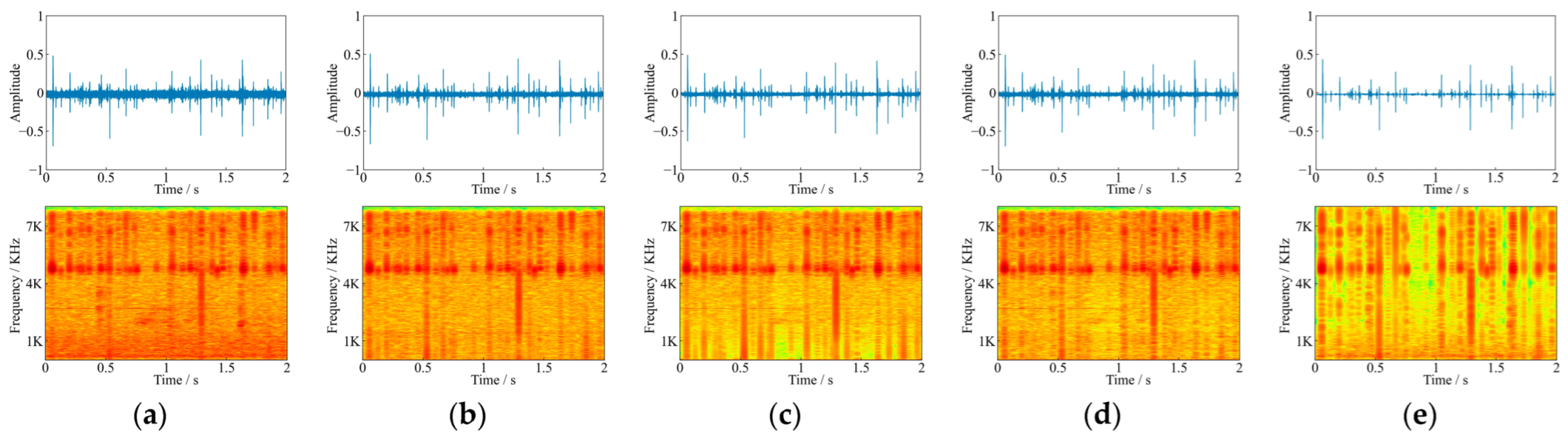
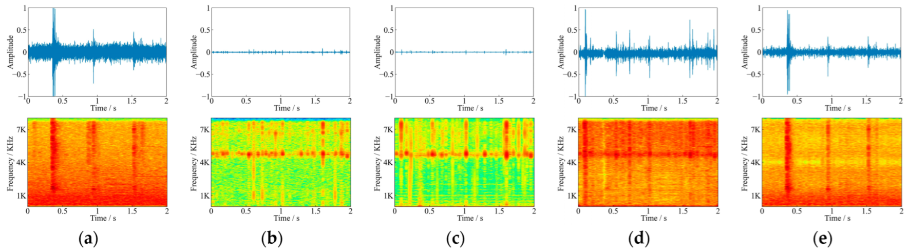
4.5. Comparisons the Acoustic Detection Effects between Noisy Sound and Denoised Sound
5. Discussion
6. Conclusions
Author Contributions
Funding
Institutional Review Board Statement
Informed Consent Statement
Data Availability Statement
Conflicts of Interest
References
- Mankin, R.; Burman, H.; Menocal, O.; Carrillo, D. Acoustic detection of Mallodon dasystomus (Coleoptera: Cerambycidae) in Persea americana (Laurales: Lauraceae) branch stumps. Fla. Entomol. 2018, 101, 321–323. [Google Scholar] [CrossRef] [Green Version]
- Rigakis, I.; Potamitis, I.; Tatlas, N.-A.; Potirakis, S.M.; Ntalampiras, S. TreeVibes: Modern tools for global monitoring of trees for borers. Smart Cities 2021, 4, 271–285. [Google Scholar] [CrossRef]
- Li, Y.; Zhao, Z.G.; Wang, T.T.; Wu, W.Q.; Wang, X.; Ma, R.Y. Application of sonic signals for fruit damage detection produced by Grapholitha molesta larval feeding. J. Shanxi Agric. Univ. Nat. Sci. Ed. 2018, 38, 13–16, 63. [Google Scholar]
- Mankin, R.; Hagstrum, D.; Guo, M.; Eliopoulos, P.; Njoroge, A. Automated applications of acoustics for stored product insect detection, monitoring, and management. Insects 2021, 12, 259. [Google Scholar] [CrossRef] [PubMed]
- Bu, Y.F.; Qi, X.J.; Wen, J.B.; Xu, Z.C. Acoustic behaviors for two species of cerambycid larvae. J. Zhejiang A F Univ. 2017, 34, 50–55. [Google Scholar]
- Zhao, Y.J.; Wei, X.Q.; Wen, J.B.; Xu, Z.C. Preliminary study on the acoustic detection of larvae Semanotus bifasciatus (Motschulsky). Ecol. Sci. 2009, 28, 242–246. [Google Scholar]
- Mankin, R.W.; Hagstrum, D.W.; Smith, M.T.; Roda, A.L.; Kairo, M. Perspective and promise: A century of insect acoustic detection and monitoring. Am. Entomol. 2011, 71, 30–44. [Google Scholar] [CrossRef]
- Luo, Q.; Wang, H.B.; Zhang, Z.; Kong, X.B. Automatic stridulation identification of bark beetles based on MFCC and BP network. J. Beijing For. Univ. 2011, 33, 81–85. [Google Scholar]
- Njoroge, A.W.; Affognon, H.; Mutungi, C.; Rohde, B.; Richter, U.; Hensel, O.; Mankin, R.W. Frequency and time pattern differences in acoustic signals produced by Prostephanus truncatus (Horn) (Coleoptera: Bostrichidae) and Sitophilus zeamais (Motschulsky) (Coleoptera: Curculionidae) in stored maize. J. Stored Prod. Res. 2016, 69, 31–40. [Google Scholar] [CrossRef]
- Yazgaç, B.G.; Kırcı, M.; Kıvan, M. Detection of sunn pests using sound signal processing methods. In Proceedings of the 2016 Fifth International Conference on Agro-Geoinformatics (Agro-Geoinformatics), Tianjin, China, 18–20 July 2016. [Google Scholar]
- Yazgaç, B.G.; Kırcı, M. Embedded system application for sunn pest detection. In Proceedings of the 2017 6th International Conference on Agro-Geoinformatics, Fairfax, VA, USA, 7–10 August 2017. [Google Scholar]
- Herrick, N.J.; Mankin, R.W. Acoustical detection of early instar Rhynchophorus ferrugineus (Coleoptera: Curculionidae) In canary island date palm, Phoenix Canariensis (Arecales: Arecaceae). Fla. Entomol. 2012, 95, 983–990. [Google Scholar] [CrossRef]
- Jalinas, J.; Güerri-Agulló, B.; Dosunmu, O.G.; Haseeb, M.; Lopez-Llorca, L.V.; Mankin, R.W. Acoustic signal applications in detection and management of Rhynchophorus spp. in fruit-crops and ornamental palms. Fla. Entomol. 2019, 102, 475–479. [Google Scholar] [CrossRef]
- Bilski, P.; Kraiewski, A.; Witomski, P.; Bobinski, P.; Lewandowski, M. Acoustic data analysis for the assessment of wood boring insects’ activity. In Proceedings of the 2018 Joint Conference-Acoustics, Ustka, Poland, 11–14 September 2018. [Google Scholar]
- Krajewski, A.; Bilski, P.; Witomski, P.; Bobiński, P.; Guz, J. The progress in the research of AE detection method of old house borer larvae (Hylotrupes bajulus L.) in wooden structures. Constr. Build. Mater. 2020, 256, 119387. [Google Scholar] [CrossRef]
- Eliopoulos, P.A.; Potamitis, I.; Kontodimas, D.C. Estimation of population density of stored grain pests via bioacoustic detection. Crop Protection 2016, 85, 71–78. [Google Scholar] [CrossRef]
- Inyang, E.I.; Hix, R.L.; Tsolova, V.; Rohde, B.B.; Dosunmu, O.; Mankin, R.W. Subterranean acoustic activity patterns of Vitacea polistiformis (Lepidoptera: Sesiidae) in relation to abiotic and biotic factors. Insects 2019, 10, 267. [Google Scholar] [CrossRef] [PubMed] [Green Version]
- Sun, Y.; Tuo, X.; Jiang, Q.; Zhang, H.; Chen, Z.; Zong, S.; Luo, Y. Drilling vibration identification technique of two pest based on lightweight neural networks. Sci. Silvae Sin. 2020, 56, 100–108. [Google Scholar]
- Liu, X.; Sun, Y.; Cui, J.; Jiang, Q.; Chen, Z.; Luo, Y. Early recognition of feeding sound of trunk borers based on artifical intelligence. Sci. Silvae Sin. 2021, 57, 93–101. [Google Scholar]
- Geng, S.L.; Li, F.J. Design of the sound insulation chamber for stored grain insect sound detection. In Applied Mechanics and Materials; Trans Tech Publications: Freienbach, Switzerland, 2012. [Google Scholar]
- Hetzroni, A.; Soroker, V.; Cohen, Y.J.C. Toward practical acoustic red palm weevil detection. Comput. Electron. Agric. 2016, 124, 100–106. [Google Scholar] [CrossRef]
- Mankin, R.W.; Al-Ayedh, H.Y.; Aldryhim, Y.; Rohde, B. Acoustic detection of Rhynchophorus ferrugineus (Coleoptera: Dryophthoridae) and Oryctes elegans (Coleoptera: Scarabaeidae) in Phoenix dactylifera (Arecales: Arecacae) trees and offshoots in Saudi Arabian orchards. J. Econ. Entomol. 2016, 109, 622–628. [Google Scholar] [CrossRef] [Green Version]
- Bilski, P.; Bobiński, P.; Krajewski, A.; Witomski, P. Detection of wood boring insects’ larvae based on the acoustic signal analysis and the artificial intelligence algorithm. Arch. Acoust. 2017, 42, 61–70. [Google Scholar] [CrossRef] [Green Version]
- Sutin, A.; Yakubovskiy, A.; Salloum, H.R.; Flynn, T.J.; Sedunov, N.; Nadel, H. Towards an automated acoustic detection algorithm for wood-boring beetle larvae (Coleoptera: Cerambycidae and Buprestidae). J. Econ. Entomol. 2019, 112, 1327–1336. [Google Scholar] [CrossRef]
- Yi, Z.K.; Tan, J.P.; Liu, S.S. A window lift motor abnormal noise classification method based on improved spectral subtraction and MFCC. Small Spec. Electr. Mach. 2017, 45, 31–38. [Google Scholar]
- Du, X.; Teng, G. Improved de-noising method of laying hens’vocalization. Trans. Chin. Soc. Agric. Mach. 2017, 48, 327–333. [Google Scholar]
- Zhao, Y.; Liu, X.; Zhang, R.; Qin, Z. Application of improved threshold wavelet denoising method in the processing of sound signal of machine tool punching. Mach. Tool Hydraul. 2020, 48, 172–175. [Google Scholar]
- Dong, H.; Liu, Z.; Ma, H.; Yan, J. Application of speech enhancement in noise-reduction from coughing pigs. J. Shanxi Agric. Univ. Nat. Sci. Ed. 2017, 37, 831–836. [Google Scholar]
- Lee, D.D.; Seung, H.S. Learning the parts of objects by nonnegative matrix factorization. Nature 1999, 401, 788–791. [Google Scholar] [CrossRef]
- Kopsinis, Y.; Mclaughlin, S. Development of EMD-based denoising methods inspired by wavelet thresholding. IEEE Trans. Sign. Process. 2009, 57, 1351–1362. [Google Scholar] [CrossRef]
- Yang, J.; Zhou, C. A fault feature extraction method based on LMD and wavelet packet denoising. Coatings 2022, 12, 156. [Google Scholar] [CrossRef]
- Xu, J.; Wang, Z.; Tan, C.; Si, L.; Liu, X. A novel denoising method for an acoustic-based system through empirical mode decomposition and an improved fruit fly optimization algorithm. Appl. Sci. 2017, 7, 215. [Google Scholar] [CrossRef] [Green Version]
- Wu, Y.; Xing, C.; Zhao, Y. Application of the sparse low-rank model in denoising of underwater acoustic signal. In Proceedings of the 2020 IEEE 3rd International Conference on Information Communication and Signal Processing (ICICSP), Shanghai, China, 12–15 September 2020. [Google Scholar]
- Fan, L.; Zhang, F.; Fan, H.; Zhang, C. Brief review of image denoising techniques. Vis. Comput. Ind. Biomed. Art 2019, 2, 1–12. [Google Scholar] [CrossRef] [Green Version]
- Li, Q.; Zhu, Z.; Xu, C.; Tang, Y. A novel denoising method for acoustic signal. In Proceedings of the 2017 IEEE International Conference on Signal Processing, Communications and Computing (ICSPCC), Xiamen, China, 22–25 October 2017. [Google Scholar]
- Shi, W.h.; Zhang, X.w.; Zou, X.; Sun, M.; Li, L. Time frequency masking based speech enhancement using deep encoder-decoder neural network. Acta Acust. 2020, 45, 299–307. [Google Scholar]
- Hui, L.; Cai, M.; Guo, C.; He, L.; Zhang, W.q.; Liu, J. Convolutional maxout neural networks for speech separation. In Proceedings of the 2015 IEEE International Symposium on Signal Processing and Information Technology (ISSPIT), Abu Dhabi, United Arab Emirates, 7–10 December 2015. [Google Scholar]
- Kolbaek, M.; Yu, D.; Tan, Z.H.; Jensen, J. Multi-talker speech separation with utterance-level permutation invariant training of deep recurrent neural networks. IEEE/ACM Trans. Audio Speech Lang. Process. 2017, 25, 1901–1913. [Google Scholar] [CrossRef] [Green Version]
- Choi, H.S.; Kim, J.H.; Huh, J.; Kim, A.; Ha, J.W.; Lee, K. Phase-aware speech enhancement with deep complex U-Net. In Proceedings of the International Conference on Learning Representations (ICLR), New Orleans, LA, USA, 6–9 May 2019. [Google Scholar]
- Jansson, A.; Humphrey, E.J.; Montecchio, N.; Bittner, R.M.; Kumar, A.; Weyde, T. Singing voice separation with deep U-Net convolutional networks. In Proceedings of the International Society for Music Information Retrieval (ISMIRC) Conference, Suzhou, China, 23–27 October 2017. [Google Scholar]
- Huang, L.; Cheng, G.; Zhang, P.; Yang, Y.; Xu, S.; Sun, J. Utterance-level permutation invariant training with latency-controlled BLSTM for single-channel multi-talker speech separation. In Proceedings of the 2019 Asia-Pacific Signal and Information Processing Association Annual Summit and Conference (APSIPA ASC), Lanzhou, China, 18–21 November 2019. [Google Scholar]
- Fu, S.; Wang, T.; Tsao, Y.; Lu, X.; Kawai, H. End-to-end waveform utterance enhancement for direct evaluation metrics optimization by fully convolutional neural networks. IEEE/ACM Trans. Audio Speech Lang. Process. 2018, 26, 1570–1584. [Google Scholar] [CrossRef] [Green Version]
- Germain, F.G.; Chen, Q.; Koltun, V. Speech denoising with deep feature losses. In Proceedings of the International Speech Communication Association, Graz, Austria, 15–19 September 2019. [Google Scholar]
- Rethage, D.; Pons, J.; Serra, X. A wavenet for speech denoising. In Proceedings of the 2018 IEEE International Conference on Acoustics, Speech and Signal Processing (ICASSP), Calgary, AB, Canada, 15–20 April 2018. [Google Scholar]
- Kim, J.H.; Yoo, J.; Chun, S.; Kim, A.; Ha, J.W. Multi-domain processing via hybrid denoising networks for speech enhancement. arXiv 2018, arXiv:1812.08914. [Google Scholar]
- Antczak, K. Deep recurrent neural networks for ECG signal denoising. arXiv 2018, arXiv:1807.11551. [Google Scholar]
- Chen, J.; Liu, M.; Xiong, P.; Meng, X.H.; Yang, L. ECG signal denoising based on convolutional auto-encoder neural network. Comput. Eng. Appl. 2020, 56, 148–155. [Google Scholar]
- Xing, Y.I.; Wang, J.; Zhao, H.B.; Zhu, L.F. Cab signal denoising process based on fully convolutional networks. J. Southwest Jiaotong Univ. 2021, 56, 444–450. [Google Scholar]
- Wang, Q.D.; Guo, L.H.; Yan, C. Underwater acoustic target waveform recovery based on deep neural networks. J. Appl. Acoust. 2019, 38, 1004–1014. [Google Scholar]
- Ephrat, A.; Mosseri, I.; Lang, O.; Dekel, T.; Wilson, K.; Hassidim, A.; Freeman, W.T.; Rubinstein, M. Looking to listen at the cocktail party: A speaker-independent audio-visual model for speech separation. ACM Trans. Gr. 2018, 37, 1–11. [Google Scholar] [CrossRef] [Green Version]
- Barker, J.; Vincent, E.; Ma, N.; Christensen, H.; Green, P. The PASCAL CHiME speech separation and recognition challenge. Comput. Speech Lang. 2013, 27, 621–633. [Google Scholar] [CrossRef] [Green Version]
- Yu, F.; Koltun, V. Multi-scale context aggregation by dilated convolutions. In Proceedings of the International Conference on Learning Representations (ICLR), San Juan, Puerto Rico, 2–4 May 2016. [Google Scholar]
- Wang, Y.X.; Narayanan, A.; Wang, D.L. On training targets for supervised speech separation. IEEE/ACM Trans. Audio Speech Lang. Process. 2014, 22, 1849–1858. [Google Scholar] [CrossRef] [Green Version]
- Giles, C.L.; Kuhn, G.M.; Williams, R.J. Dynamic recurrent neural networks: Theory and applications. IEEE Trans. Neural Netw. 1994, 5, 153–156. [Google Scholar] [CrossRef]
- Cho, K.; Merrienboer, B.V.; Gulcehre, C.; Ba Hdanau, D.; Bougares, F.; Schwenk, H.; Bengio, Y. Learning phrase representations using RNN encoder-decoder for statistical machine translation. arXiv 2014, arXiv:1406.1078. [Google Scholar]
- Hochreiter, S.; Schmidhuber, J. Long short-term memory. Neural Comput. 1997, 9, 1735–1780. [Google Scholar] [CrossRef] [PubMed]
- Schuster; Mike; Paliwal; Kuldip, K. Bidirectional recurrent neural networks. IEEE Trans. Sign. Process. 1997, 45, 2673–2681. [Google Scholar] [CrossRef] [Green Version]
- Hansen, J.; Pellom, B. An effective quality evaluation protocol for speech enhancement algorithms. In Proceedings of the International Conference on Spoken Language Processing (ICSLP), Sidney, NSW, Australia, 30 November–4 December 1998. [Google Scholar]
- Cohen, I. Analysis of two-channel generalized sidelobe canceller (GSC) with post-filtering. IEEE Trans. Speech Audio Process. 2003, 11, 684–699. [Google Scholar] [CrossRef]
- Donoho, D.L.; Johnstone, I.M. Ideal spatial adaptation by wavelet shrinkage. Biometrika 1994, 81, 425–455. [Google Scholar] [CrossRef]
- Chung, J.S.; Nagrani, A.; Zisserman, A. VoxCeleb2: Deep speaker recognition. In Proceedings of the INTERSPEECH, Hyderabad, India, 2–6 September 2018. [Google Scholar]


| Category | Training | Test | ||
|---|---|---|---|---|
| Audio Segments | Audio Slices | Audio Segments | Audio Slices | |
| S.bifasciatus feeding sounds | 42 | 6300 | 18 | 2700 |
| Environmental noises | 42 | 6300 | 18 | 2700 |
| Total | 84 | 12,600 | 36 | 5400 |
| Models | Average ΔSNR (dB) | Average ΔSegSNR (dB) | Average LSD (dB) |
|---|---|---|---|
| TDD-Net-C | 14.40 | 15.68 | 0.96 |
| TDD-Net-D | 16.97 | 18.13 | 0.87 |
| TDD-Net-DS | 17.24 | 18.35 | 0.81 |
| TDD-Net-DC | 17.53 | 18.59 | 0.85 |
| Models | Average ΔSNR (dB) | Average ΔSegSNR (dB) | Average LSD (dB) |
|---|---|---|---|
| FDD-Net-R | 7.58 | 8.50 | 1.60 |
| FDD-Net-G | 9.23 | 10.34 | 1.01 |
| FDD-Net-L | 9.52 | 10.41 | 0.95 |
| FDD-Net-BR | 10.22 | 11.53 | 1.24 |
| FDD-Net-BG | 10.85 | 12.06 | 0.95 |
| FDD-Net-BL | 11.10 | 12.04 | 0.84 |
| # | Layer | Parameters | Activation |
|---|---|---|---|
| 1 | Convolution (3 × 3) | Filter size = 32, Stride = 2 | ReLU |
| 2 | Convolution (3 × 3) | Filter size = 64, Stride = 2 | ReLU |
| 4 | Global Average Pooling | ||
| 5 | Fully connected | Size = 3 | Softmax |
Publisher’s Note: MDPI stays neutral with regard to jurisdictional claims in published maps and institutional affiliations. |
© 2022 by the authors. Licensee MDPI, Basel, Switzerland. This article is an open access article distributed under the terms and conditions of the Creative Commons Attribution (CC BY) license (https://creativecommons.org/licenses/by/4.0/).
Share and Cite
Liu, X.; Zhang, H.; Jiang, Q.; Ren, L.; Chen, Z.; Luo, Y.; Li, J. Acoustic Denoising Using Artificial Intelligence for Wood-Boring Pests Semanotus bifasciatus Larvae Early Monitoring. Sensors 2022, 22, 3861. https://0-doi-org.brum.beds.ac.uk/10.3390/s22103861
Liu X, Zhang H, Jiang Q, Ren L, Chen Z, Luo Y, Li J. Acoustic Denoising Using Artificial Intelligence for Wood-Boring Pests Semanotus bifasciatus Larvae Early Monitoring. Sensors. 2022; 22(10):3861. https://0-doi-org.brum.beds.ac.uk/10.3390/s22103861
Chicago/Turabian StyleLiu, Xuanxin, Haiyan Zhang, Qi Jiang, Lili Ren, Zhibo Chen, Youqing Luo, and Juhu Li. 2022. "Acoustic Denoising Using Artificial Intelligence for Wood-Boring Pests Semanotus bifasciatus Larvae Early Monitoring" Sensors 22, no. 10: 3861. https://0-doi-org.brum.beds.ac.uk/10.3390/s22103861