3D Vision by Using Calibration Pattern with Inertial Sensor and RBF Neural Networks

Abstract
:1. Introduction
2. Artificial Neural Networks (ANNs)
2.1. Training of Radial Basis Function Neural Networks
- ‖…‖ : Euclidean norm,
- cε : The center,
- σε : The width of the εth neuron in the hidden layer,
- wi,ε : The weights in the output layer,
- N : The number of Gaussian neurons in the hidden layer,
- λ : Input pattern of RBF,
- δ : Output pattern of RBF,
- I : The number of neurons in the output layer.
3. Proposed Method
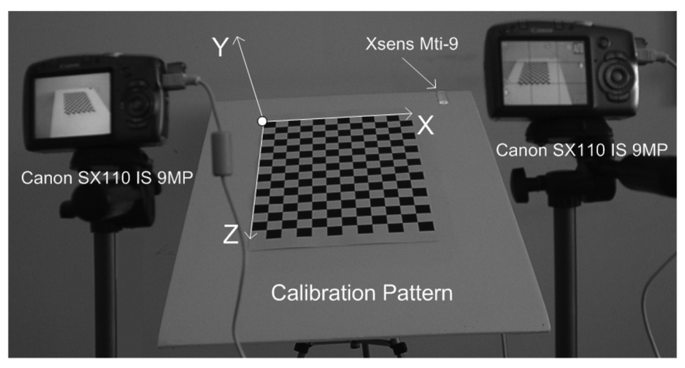
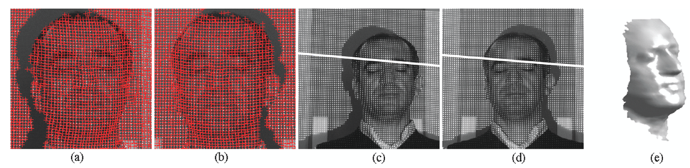
- Training Data Arrangement for RBF: In this step, the calibration grid-pattern has been arbitrarily rotated towards the cameras around the static-fixed axis in five approximately equal steps and the stereo images have been captured with two static cameras at the end of each rotation. There are 219 grid-corners on the calibration pattern and totally 1,095 grid-corners have been observed. The number of randomly selected observations of grid-corners have been used as 795 (which is the value of Nt in Equation 2) for the training set of RBF and the remaining 300 observations of grid-corners have been used for the generalization test set of RBF.In the case of rotating the calibration plane arbitrarily without a fixed axis in calibration space, both the spatial translations and spatial rotations must be observed, in order to compute the exact position of 3D grid corners on calibration pattern in 3D space. In order to avoid additional observation parameters (i.e., spatial translations), a fixed axis has been used in this paper.The rotation matrix of calibration grid-pattern has been acquired at 100 Hz by using an Xsens MTi-9 sensor attached to calibration pattern. The object reset function of the SDK of Xsens aims to facilitate aligning the MTi-9 sensor coordinate frame with the 3D global coordinate frame of the calibration grid-pattern to which the sensor is attached. Therefore, the object reset function has been applied to Xsens MTi-9 sensor by using the related SDK in Matlab before each measurement in order to control the drift-error of the related sensor.The calibration pattern is assumed to be vertical at its initial position. Since an object reset function has been applied to Xsens MTi-9 sensor at initial position of the calibration pattern, the values of initial rotations of the calibration pattern are equal to zero.The global coordinates of the corners of calibration grid-pattern at its initial position have been manually detected according to the global origin illustrated in Figure 1. The global origin is static in each image and the checkerboard points are fixed relative to the static global origin. The sizes of the grids on the calibration pattern are equal to 30-by-30 mm. The corners of the calibration grid-pattern have the value of Y = 0 at the initial position of the calibration grid-pattern. The corresponding global coordinates (X, Y, Z) of (uleft, vleft, uright, vright) have been computed by multiplying the related spatial coordinates of corners with the related rotation matrix.Xsens MTi-9 is affected by excessive shocks, violent handling, magnetic fields and thermal-effects. Therefore, all the sensor measurements have been realized by using the default Kalman filter of SDK of the related sensor, in order to suppress the effects of the mentioned noise sources over measurements.The Harris Corner Detection operator [30] has been used to extract the image coordinates of the corners of calibration grid-pattern as Harris-points. The feature correspondence problem has been solved by computing the homography of stereo images (Figure 2) using the related Harris-points (Figure 2 a,b) and Ransac algorithm [31]. Since the stereo matching problem could be solved efficiently, epipolar lines have been extracted successfully before image-matching operations (as in Figure 2 c,d). The normalized cross correlation operator has been applied to stereo images, in order to obtain image coordinates of corners (uleft, vleft, uright, vright) of calibration grid-pattern, where (uleft, vleft), (uright, vright) denotes the image coordinates of the related corners in the left and right stereo images, respectively.
- Training of RBF: The proposed method uses a 3-layered RBF neural network in order to map 2-by-2D image coordinates to 3D global coordinates. The input layer of RBF has four-inputs for the left and right image coordinates (uleft, vleft, uright, vright) of the observed point; and the output layer of RBF has three-neurons that correspond to the global coordinates of the related point. The RBF has been trained as explained in Section 2.1. The test error of RMS-fitness function is 0.017 and has been computed as seen in Table 1.
- 3D Reconstruction of Test Object: In this step, a predefined texture pattern has been projected onto the test object (i.e., The face of Author) located inside the motion-volume of rotating-plane by using a DLP data projector. The stereo image coordinates of the projected texture pattern have been acquired from the rectified images by using normalized cross correlation. The obtained stereo image coordinates have been applied to the trained-RBF, in order to compute the corresponding global coordinates, [X Y Z]test.The noises within the computed global coordinates, which are affected from image-matching errors, have been eliminated by using the FastRBF toolbox [32].Surface meshing and mesh smoothing have been intensively used in 3D visualization applications. The FastRBF toolbox offers several techniques for fitting radial based functions to measured data including error-bar fitting, spline smoothing and linear filtering. In this paper, the linear filtering technique of RBF has been used. FastRBFs implicit surface meshing and mesh smoothing tools are particularly useful for reconstructing surfaces from point cloud range data. Therefore, the FastRBF tools have been used in mesh generation and smoothing of the author's face, illustrated in Figure 2(e).
3.1. Modified Direct Linear Transformation
3.2. The Camera Model
- (xu, yu) : lens-distorted image coordinates
- (x0, y0) : image coordinates of principal point
- (fx, fy) : focal lengths
- (m11, m12,…, m33) : elements of rotation matrix
- (X0, Y0, Z0) : global coordinates of projection center
3.3. Xsens MTi-9 Inertial Sensor
4. Experiments
5. Results and Discussion
- The proposed method introduces a novel implicit camera calibration method based on inertial sensors (Implicit camera calibration techniques are not interested in the physical parameters of the cameras).
- The results of the proposed method are close to MDLT but they are better, therefore it can be used in robotic vision as MDLT.
- The computational-burden of the proposed method is less than MDLT.
- The required time for preparation and scaling of the 2D calibration object of the proposed method is less than the time of preparation and scaling of the 3D calibration object of MDLT.
- It offers high accuracy both in planimetric (x,y) and in depth (z).
- It is simple to apply and fast after training.
- The image distortion and the physical parameters of the cameras have been covered by the neural network model of the proposed method.
- No image distortion model is required.
- It does not use physical parameters of cameras.
- An approximated solution for initial step of camera calibration is not employed.
- Optimization algorithms are not employed during 3D reconstruction in contrary to some of the well-known 3D acquisition methods.
Acknowledgments
References and Notes
- Anchini, R.; Liguori, C.; Paciello, V.; Paolillo, A. A Comparison Between Stereo-Vision Techniques for The Reconstruction of 3-D Coordinates of Objects. IEEE Trans. Instrum. Meas. 2006, 55, 1459–1466. [Google Scholar]
- Available online: http://www.vision.caltech.edu/bouguetj/calib_doc/ (accessed 10 April 2009).
- Lv, F.; Zhao, T.; Nevatia, R. Camera Calibration From Video of a Walking Human. IEEE Trans. Pattern Anal. Mach. Intell. 2006, 28, 1513–1518. [Google Scholar]
- Wang, F.Y. An Efficient Coordinate Frame Calibration Method for 3-D Measurement by Multiple Camera Systems. IEEE Trans. Syst., Man, Cybern. C, Appl. Rev. 2005, 35, 453–464. [Google Scholar]
- Hu, W.; Hu, M.; Zhou, X.; Tan, T.; Lou, J.; Maybank, S. Principal Axis-Based Correspondence Between Multiple Cameras for People Tracking. IEEE Trans. Pattern Anal. Mach. Intell. 2006, 28, 663–671. [Google Scholar]
- Wilczkowiak, M.; Sturm, P.; Boyer, E. Using Geometric Constraints Through Parallelepipeds for Calibration and 3D Modeling. IEEE Trans. Pattern Anal. Mach. Intell. 2005, 27, 194–207. [Google Scholar]
- Zhao, Z.; Liu, Y.; Zhang, Z. Camera Calibration With Three Noncollinear Points Under Special Motions. IEEE Trans. Image Process. 2008, 17, 2393–2402. [Google Scholar]
- Malm, H.; Heyden, A. Extensions Of Plane-Based Calibration To The Case of Translational Motion in a Robot Vision Setting. IEEE Trans. Robot. 2006, 22, 322–333. [Google Scholar]
- Vincent, C.Y.; Tjahjadi, T. Multiview Camera-Calibration Framework For Nonparametric Distortions Removal. IEEE Trans. Robot. 2005, 21, 1004–1009. [Google Scholar]
- Akella, M.R. Vision-Based Adaptive Tracking Control of Uncertain Robot Manipulators. IEEE Trans. Robot. 2005, 21, 747–753. [Google Scholar]
- Zhang, H.; Wong, K.Y.K.; Zhang, G. Camera Calibration From Images of Spheres. IEEE Trans. Pattern Anal. Mach. Intell. 2007, 29, 499–502. [Google Scholar]
- Cao, X; Foroosh, H. Camera Calibration Using Symmetric Objects. IEEE Trans. Image Process. 2006, 15, 3614–3619. [Google Scholar]
- Kannala, J.; Brandt, S.S. A Generic Camera Model and Calibration Method for Conventional, Wide-Angle, and Fish-Eye Lenses. IEEE Trans. Pattern Anal. Mach. Intell. 2006, 28, 1335–1340. [Google Scholar]
- Okatani, T.; Deguchi, K. Autocalibration Of a Projector-Camera System. IEEE Trans. Pattern Anal. Mach. Intell. 2005, 27, 1845–1855. [Google Scholar]
- Nedevschi, S.; Vancea, C.; Marita, T.; Graf, T. Online Extrinsic Parameters Calibration for Stere-ovision Systems Used in Far-Range Detection Vehicle Applications. IEEE Trans. Intell. Transp. Syst. 2007, 8, 651–660. [Google Scholar]
- Chen, I.H.; Wang, S.J. An Efficient Approach For Dynamic Calibration Of Multiple Cameras. IEEE Trans. Autom. Sci. Eng. 2009, 6, 187–194. [Google Scholar]
- Tien, F.C.; Chang, C.A. Using Neural Networks for 3D Measurement in Stereo Vision Inspection Systems. Int. J. Prod. Res. 1999, 37, 1935–1948. [Google Scholar]
- Cuevas, F.J.; Servin, M.; Rodriguez-Vera, R. Depth Object Recovery Using Radial Basis Functions. Opt. Commun. 1999, 163, 270–277. [Google Scholar]
- Memony, Q.; Khan, S. Camera Calibration and Three-Dimensional World Reconstruction of Stereo-Vision Using Neural Networks. J. Syst. Sci. Syst. Eng. 2001, 32, 1155–1159. [Google Scholar]
- Xsens, Co. Mti and Mtx User Manual and Technical Documentation; Netherlands, 2009; Volume MT0137P, pp. 2–30. [Google Scholar]
- Available online: http://www.xsens.com/ (accessed 10 April 2009).
- Lobo, J.; Dias, J. Fusing of Image and Inertial Sensing for Camera Calibration. International Conference on Multisensor Fusion and Integration for Intelligent Systems, Baden-Baden, Germany, August, 2001; pp. 103–108.
- Randeniya, D.I.B.; Gunaratne, M.; Sarkar, S.; Nazef, A. Calibration of Inertial and Vision Systems as a Prelude To Multi-Sensor Fusion. Transport. Res. C 2008, 16, 255–274. [Google Scholar]
- Hatze, H. High-Precision Three-Dimensional Photogrammetric Calibration and Object Space Reconstruction Using a Modified DLT-Approach. J. Biomech. 1988, 21, 533–538. [Google Scholar]
- Graupe, D. Principles of Artificial Neural Networks; World Scientific Publishing Company: Singapore, 2007; ISBN: ISBN: 9812706240. [Google Scholar]
- Simon, D. Training Radial Basis Neural Networks with The Extended Kalman Filter. Neurocomputing 2002, 48, 455–475. [Google Scholar]
- Chen, J.Y.; Qin, Z. Training Rbf Neural Networks with Pso and Improved Subtractive Clustering Algorithms. Letc. Note. Comput. Sci. 2006, 4233, 1148–1155. [Google Scholar]
- Redondo, M.F.; Sospedra, J.T.; Espinosa, C.H. Training Rbfs Networks: A Comparison Among Supervised and Not Supervised Algorithms. Letc. Note. Comput. Sci. 2006, 4232, 477–486. [Google Scholar]
- Storn, R.; Price, K. Differential Evolution - A Simple and Efficient Heuristic for Global Optimization Over Continuous Spaces. J. Global Optim. 1997, 11, 341–359. [Google Scholar]
- Harris, C.; Stephens, M. A Combined Corner and Edge Detector. Proceedings of the Alvey Vision Conference, Manchester, Uk, August 31-September 2, 1988; pp. 147–151.
- Fischler, M.A.; Bolles, R.C. Random Sample Consensus: A Paradigm for Model Fitting with Applications To Image Analysis and Automated Cartography. Commun. ACM 1981, 24, 381–395. [Google Scholar]
- Available online: http://www.farfieldtechnology.com/products/toolbox/ (accessed 10 April 2009).


| Fitness Function | Equation | Test Error | N of Equation 1 |
|---|---|---|---|
| RMS | 0.017 | 24 | |
| MSE | 0.019 | 25 | |
| SSE | 0.021 | 25 | |
| MAE | 0.033 | 28 |
| Parameter | Camera #1 | Camera #2 |
|---|---|---|
| fx | 1649.149 | 1650.865 |
| fy | 1655.941 | 1658.082 |
| x0 | 789.515 | 794.803 |
| y0 | 582.668 | 581.167 |
| Sx | 0.000 | 0.000 |
| k1 | -0.210 | -0.211 |
| k2 | 0.175 | 0.186 |
| k3 | -0.001 | -0.002 |
| k4 | 0.000 | 0.000 |
| k5 | 0.000 | 0.000 |
| Method | MSE | ||
|---|---|---|---|
| X (cm) | Y (cm) | Z (cm) | |
| Proposed (with original measurements) | 0.07104 | 0.25692 | 0.09343 |
| MDLT (with original measurements) | 0.08193 | 0.34160 | 0.11131 |
| Proposed (with denoised measurements) | 0.00085 | 0.00495 | 0.00109 |
| MDLT (with denoised measurements) | 0.00193 | 0.01028 | 0.00277 |
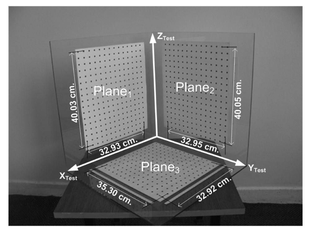
| Reference Measurements | MDLT | Proposed Method | ||||
|---|---|---|---|---|---|---|
| Plane No | Edge #1 | Edge #2 | Edge #1 | Edge #2 | Edge #1 | Edge #2 |
| 1 | 40.03 | 32.93 | 39.9336 | 32.9682 | 40.0277 | 32.9519 |
| 2 | 40.05 | 32.95 | 40.0378 | 32.9208 | 40.0239 | 32.9591 |
| 3 | 35.30 | 32.92 | 35.3193 | 32.9670 | 35.2859 | 32.9557 |
© 2009 by the authors; licensee Molecular Diversity Preservation International, Basel, Switzerland. This article is an open access article distributed under the terms and conditions of the Creative Commons Attribution license (http://creativecommons.org/licenses/by/3.0/).
Share and Cite
Beşdok, E. 3D Vision by Using Calibration Pattern with Inertial Sensor and RBF Neural Networks. Sensors 2009, 9, 4572-4585. https://0-doi-org.brum.beds.ac.uk/10.3390/s90604572
Beşdok E. 3D Vision by Using Calibration Pattern with Inertial Sensor and RBF Neural Networks. Sensors. 2009; 9(6):4572-4585. https://0-doi-org.brum.beds.ac.uk/10.3390/s90604572
Chicago/Turabian StyleBeşdok, Erkan. 2009. "3D Vision by Using Calibration Pattern with Inertial Sensor and RBF Neural Networks" Sensors 9, no. 6: 4572-4585. https://0-doi-org.brum.beds.ac.uk/10.3390/s90604572