
Pooling Bio-Specimens in the Presence of Measurement Error and Non-Linearity in Dose-Response: Simulation Study in the Context of a Birth Cohort Investigating Risk Factors for Autism Spectrum Disorders

Abstract
:1. Introduction
2. Material and Methods
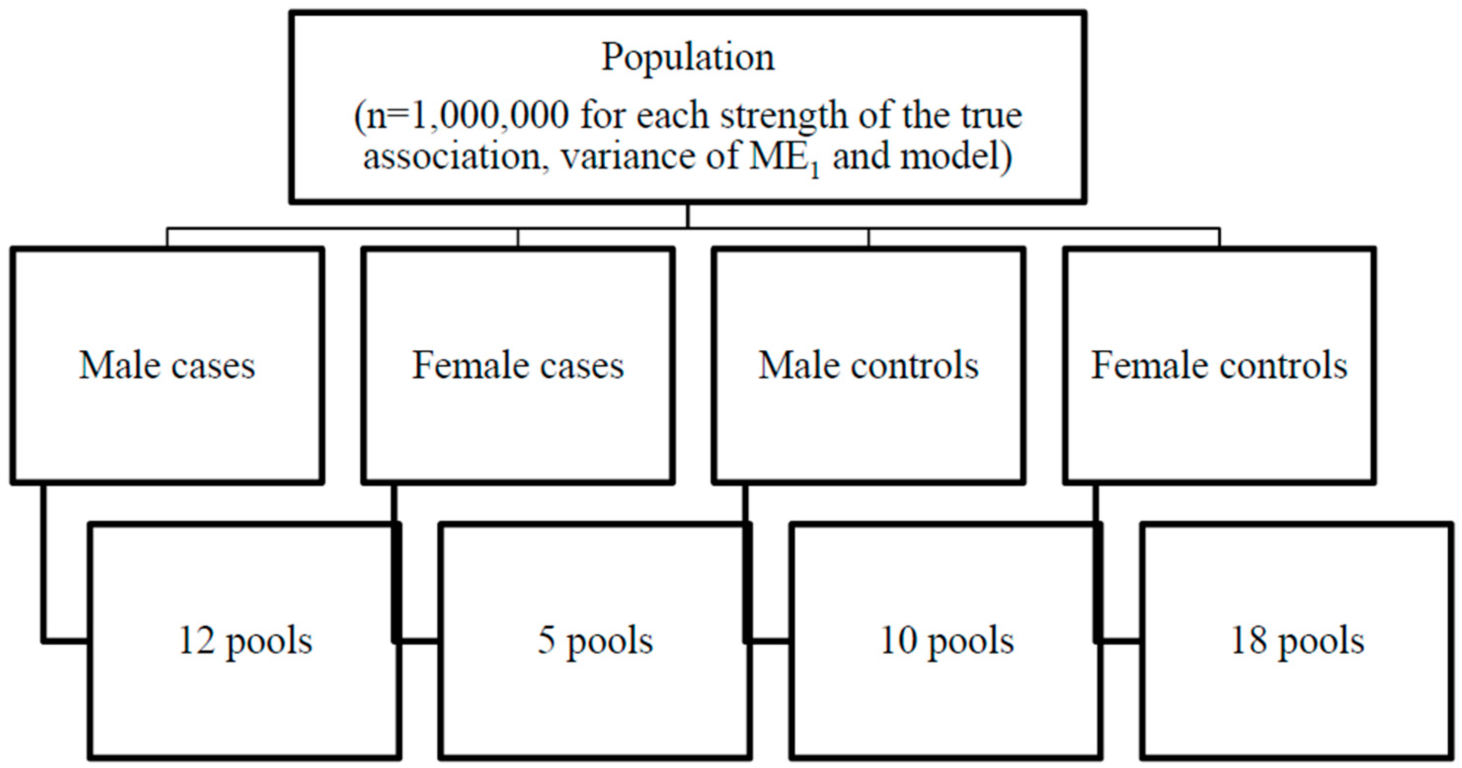
2.1. Simulated Population
2.2. Covariate Measurement Error

| Values in the Population (Notation) | True Values | Observed Values | Measurement Error | Postulated True Association with Latent Measure of Outcome a | Cutoff Used for Dichotomization |
|---|---|---|---|---|---|
| Environmental exposure 1 (X1) | X1~N(0,1), correlated with X2 by Pearson correlation ρ = 0.7 | W1 = X1 + ε1 | ε1~N(0,σ2), where σ2 ∈ {0.0625, 0.25, 1} | {0.15, 0.25, 0.5} | |
| Environmental exposure 2 (X2) | X2~N(0,1), correlated with X1 by Pearson correlation ρ = 0.7 | W2 = X2 + ε2 | ε2~N(0,0.25) | 0 | |
| Sex (Z) | Z~Binomial(0.5, 1) | Z | None | 1 | |
| Gestational age (Xga) | Xga ~ (43 – χ2(3)) 1 week was subtracted from the above gestational age for 5% of males | Wga = R((Wga + εga); 23, 43), Where R(.) is a function that is the rounded expression to integers, and then truncated to 23 to 43 weeks. | 0.1 | ||
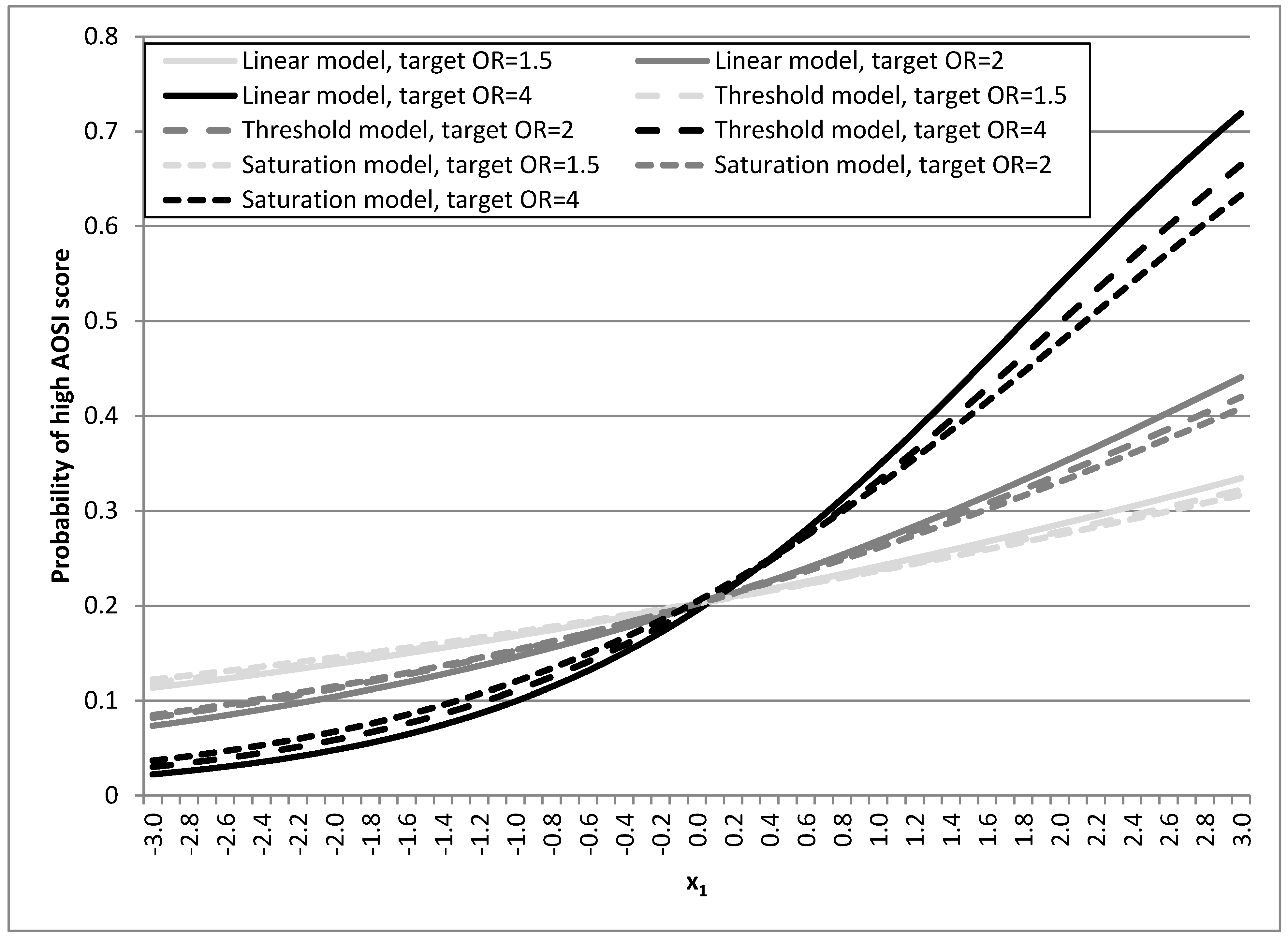
| Autism endophenotype (latent, Y) | εy~N(0,1) Linear model YL = β1X1 + β3Z + β4Xga + εy, Semi-linear model 1: threshold model If x1 < −1 then YT = β3Z+ β4Xga + εy If x1 ≥ −1 then YT = 1.5 × β1X1 + β3Z + β4Xga + εy Semi-linear model 2: saturation model If x1 <−1 then YS =1.5 × β1X1 + β3Z + β4Xga + εy If x1 ≥ −1 then YS = 0.5 × β1X1 + β3Z + β4Xga + εy, | Y* = R(T(y); 0, 18), where T(.) is a function that is transformed to the Y log-normal distribution that match observed AOSI in EARLI | due to rounding by R(.) b | Not applicable | 0–6, 7–18 |
2.3. Linear and Semi-Linear Risk Models
2.4. Case Definition and Outcome Misclassification
2.5. Pool Construction and Composition and Simulated Cohorts

2.6. Assessing the Effect of Pooling
2.7. Comparison of the Replicates to the Population
2.8. Comparison of the Individual Level Replicate Analysis and Pools of Different Sizes
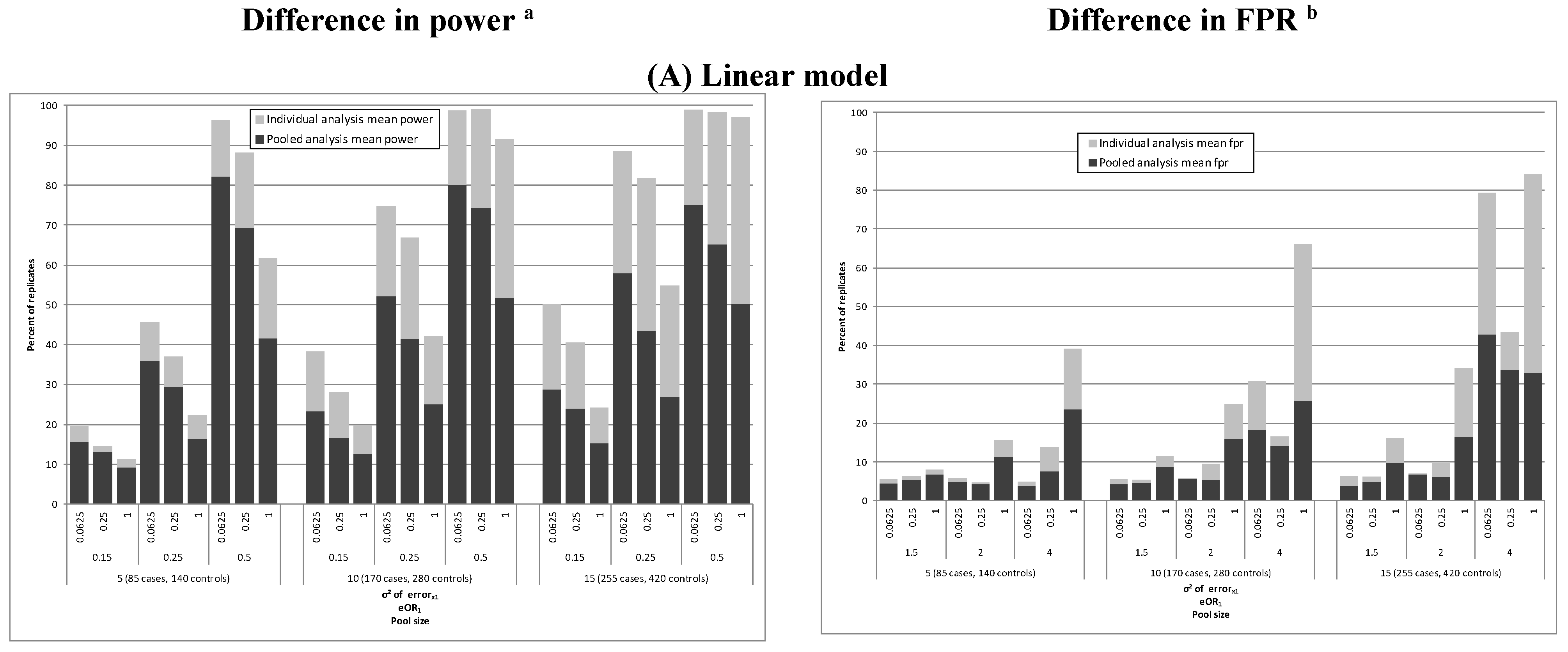
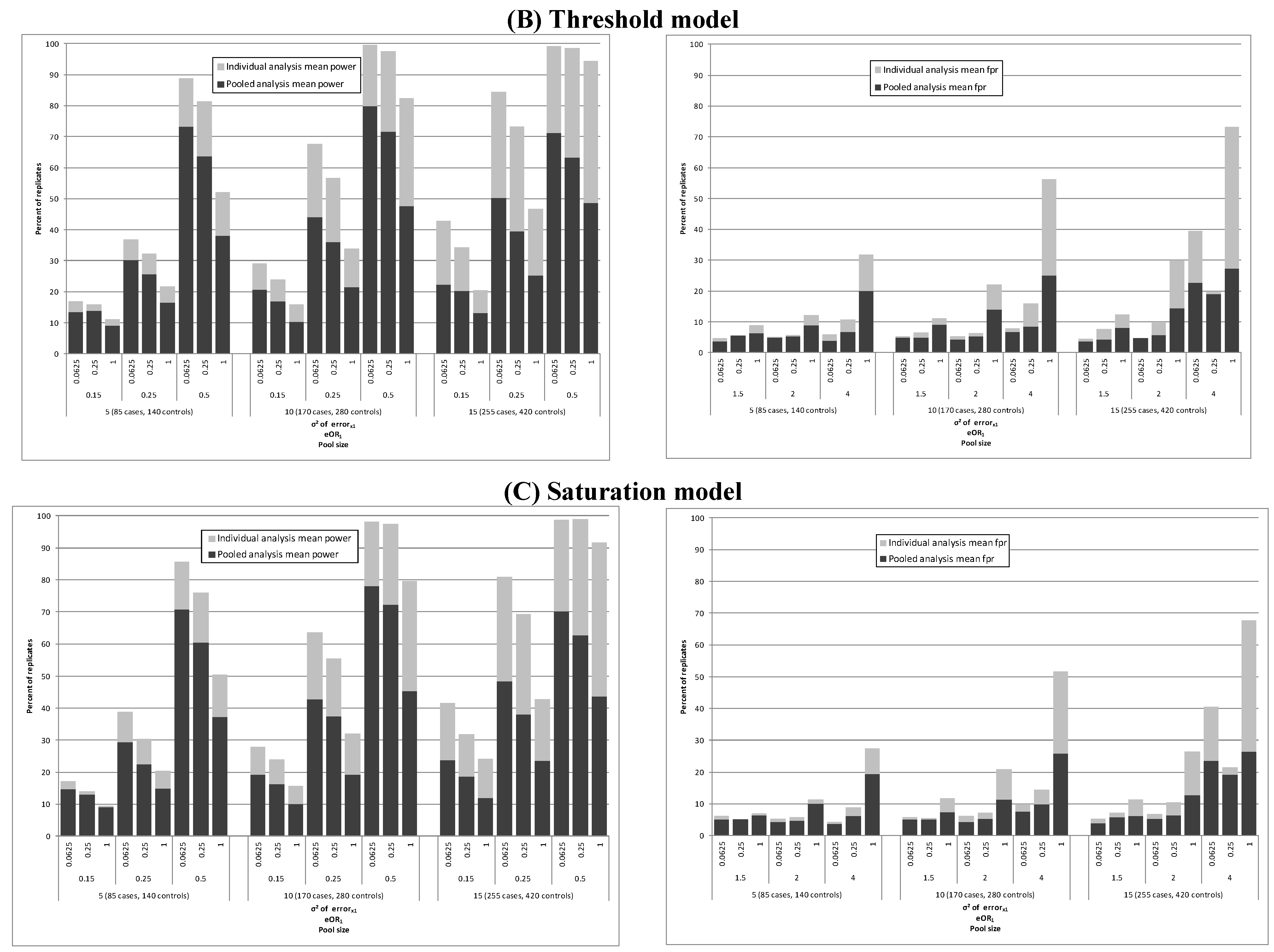
3. Results

| Cohort (Pool) Size | eOR1 (eβ1) | (σ2) | Comparison to Population Analysis | Comparison to Individual Level Replicate Analysis | |||
|---|---|---|---|---|---|---|---|
| Exposure 1 | Exposure 2 | % Mean Change in OR d | |||||
| Power a (%) | Bias b | FPR c (%) | Exposure 1 | Exposure 2 | |||
| Linear model | |||||||
| 225 (5) | 1.5 (0.15) | Truth e | 26.3–27.5 | 1.1 | 3.1–3.6 | ||
| 0.0625 | 15.7 | 1.1 | 4.4 | 3.2 | 0.0 | ||
| 0.25 | 13.1 | 1.0 | 5.4 | 2.7 | 0.2 | ||
| 1 | 9.3 | 0.9 | 6.8 | 1.2 | 1.1 | ||
| 2.0 (0.25) | Truth e | 60.8–63.3 | 1.1 | 5.7–6.5 | |||
| 0.0625 | 36.0 | 1.1 | 4.8 | 6.1 | −0.8 | ||
| 0.25 | 29.4 | 1.0 | 4.2 | 4.3 | 0.5 | ||
| 1 | 16.6 | 0.8 | 11.4 | 2.4 | 2.4 | ||
| 4.0 (0.5) | Truth e | 98.7–98.9 | 1.3 | 10.6–12.3 | |||
| 0.0625 | 82.1 | 1.3 | 3.9 | 13.6 | 0.2 | ||
| 0.25 | 69.3 | 1.0 | 7.6 | 10.8 | 1.9 | ||
| 1 | 41.5 | 0.7 | 23.6 | 6.0 | 4.0 | ||
| 450 (10) | 1.5 (0.15) | Truth e | 40.3–41.6 | 1.1 | 3.7–4.1 | ||
| 0.0625 | 23.3 | 1.1 | 4.2 | 3.9 | −0.7 | ||
| 0.25 | 16.8 | 1.0 | 4.7 | 2.9 | 0.5 | ||
| 1 | 12.5 | 0.9 | 8.7 | 1.9 | 1.5 | ||
| 2.0 (0.25) | Truth e | 82.0–83.4 | 1.1–1.2 | 7.8–8.6 | |||
| 0.0625 | 52.1 | 1.1 | 5.5 | 8.3 | −1.0 | ||
| 0.25 | 41.4 | 1.0 | 5.3 | 7.2 | 0.3 | ||
| 1 | 25.0 | 0.8 | 15.8 | 3.6 | 3.9 | ||
| 4.0 (0.5) | Truth e | 92.9–93.6 | 1.4 | 16.6–18.3 | |||
| 0.0625 | 80.2 | 1.3 | 18.4 | 16.2 | −0.7 | ||
| 0.25 | 74.2 | 1.1 | 14.2 | 16.6 | 2.0 | ||
| 1 | 51.8 | 0.7 | 25.7 | 10.1 | 6.6 | ||
| 675 (15) | 1.5 (0.15) | Truth e | 48.3–50.5 | 1.1 | 4.9–5.0 | ||
| 0.0625 | 28.8 | 1.1 | 3.9 | 5.4 | −0.8 | ||
| 0.25 | 24.0 | 1.0 | 4.8 | 5.1 | −1.1 | ||
| 1 | 15.3 | 0.9 | 9.7 | 2.8 | 1.3 | ||
| 2.0 (0.25) | Truth e | 87.8–89.4 | 1.2 | 9.4–11.3 | |||
| 0.0625 | 57.9 | 1.2 | 6.7 | 11.2 | −0.2 | ||
| 0.25 | 43.5 | 1.1 | 6.1 | 9.0 | 0.7 | ||
| 1 | 26.9 | 0.8 | 16.5 | 4.5 | 3.7 | ||
| 4.0 (0.5) | Truth e | 82.2–84.9 | 1.3–1.4 | 15.3–16.8 | |||
| 0.0625 | 75.2 | 1.4 | 42.8 | 18.3 | −2.9 | ||
| 0.25 | 65.1 | 1.1 | 33.8 | 17.0 | 2.3 | ||
| 1 | 28.8 | 0.7 | 12.2 | 0.1 | 0.1 | ||
| Threshold model | |||||||
| 225 (5) | 1.5 (0.15) | Truth e | 22.6–24.4 | 1.1 | 2.9-3.3 | ||
| 0.0625 | 13.4 | 1.1 | 3.6 | 2.9 | −0.1 | ||
| 0.25 | 13.9 | 1.0 | 5.6 | 2.8 | −0.1 | ||
| 1 | 9.1 | 0.9 | 6.3 | 1.2 | 0.4 | ||
| 2.0 (0.25) | Truth e | 50.8–54.4 | 1.1 | 4.3–4.8 | |||
| 0.0625 | 30.1 | 1.1 | 5.0 | 5.0 | −0.9 | ||
| 0.25 | 25.7 | 1.0 | 5.3 | 4.2 | 0.1 | ||
| 1 | 16.5 | 0.9 | 8.9 | 2.4 | 1.8 | ||
| 4.0 (0.5) | Truth e | 96.4–96.9 | 1.2–1.3 | 7.8-8.8 | |||
| 0.0625 | 73.2 | 1.2 | 3.8 | 9.4 | −0.9 | ||
| 0.25 | 63.8 | 1.0 | 6.8 | 7.9 | 0.8 | ||
| 1 | 38.1 | 0.7 | 20.1 | 4.4 | 3.3 | ||
| 450 (10) | 1.5 (0.15) | Truth e | 36.5–36.7 | 1.1 | 3.4–3.6 | ||
| 0.0625 | 20.6 | 1.1 | 4.8 | 3.1 | 0.0 | ||
| 0.25 | 17.0 | 1.0 | 4.9 | 2.9 | 0.4 | ||
| 1 | 10.3 | 0.9 | 9.0 | 1.7 | 1.2 | ||
| 2.0 (0.25) | Truth e | 73.5–76.2 | 1.1 | 6.1–6.9 | |||
| 0.0625 | 44.0 | 1.1 | 4.3 | 6.6 | 0.3 | ||
| 0.25 | 35.9 | 1.0 | 5.3 | 6.0 | 0.9 | ||
| 1 | 21.5 | 0.8 | 14.1 | 3.2 | 2.2 | ||
| 4.0 (0.5) | Truth e | 95.0–97.1 | 1.2–1.3 | 10.8–11.5 | |||
| 0.0625 | 79.8 | 1.2 | 6.7 | 12.7 | −0.8 | ||
| 0.25 | 71.6 | 1.0 | 8.4 | 11.2 | 1.6 | ||
| 1 | 47.5 | 0.7 | 25.1 | 6.8 | 5.2 | ||
| 675 (15) | 1.5 (0.15) | Truth e | 42.9–43.9 | 1.1 | 4.2–4.6 | ||
| 0.0625 | 22.3 | 1.1 | 3.7 | 4.9 | −1.0 | ||
| 0.25 | 20.2 | 1.0 | 4.3 | 3.9 | −0.5 | ||
| 1 | 13.2 | 0.9 | 8.0 | 2.0 | 1.2 | ||
| 2.0 (0.25) | Truth e | 80.8–83.1 | 1.2 | 7.5–8.5 | |||
| 0.0625 | 50.3 | 1.1 | 4.6 | 8.4 | −0.6 | ||
| 0.25 | 39.5 | 1.0 | 5.8 | 6.6 | 1.4 | ||
| 1 | 25.3 | 0.9 | 14.5 | 3.8 | 3.5 | ||
| 4.0 (0.5) | Truth e | 85.0–86.9 | 1.3 | 12.2–13.3 | |||
| 0.0625 | 71.2 | 1.3 | 22.8 | 15.8 | −3.5 | ||
| 0.25 | 63.4 | 1.0 | 19.0 | 11.8 | 3.8 | ||
| 1 | 48.7 | 0.8 | 27.3 | 8.3 | 5.9 | ||
| Saturation model | |||||||
| 225 (5) | 1.5 (0.15) | Truthe | 19.4–22.5 | 1.0–1.1 | 2.3–3.5 | ||
| 0.0625 | 14.6 | 1.1 | 5.2 | 3.4 | 0.1 | ||
| 0.25 | 12.9 | 1.0 | 5.1 | 2.8 | −0.8 | ||
| 1 | 9.0 | 0.9 | 6.3 | 0.8 | −0.1 | ||
| 2.0 (0.25) | Truth e | 49.7–52.7 | 1.1 | 4.7–5.4 | |||
| 0.0625 | 29.4 | 1.1 | 4.3 | 4.7 | −0.2 | ||
| 0.25 | 22.6 | 1.0 | 4.6 | 3.8 | 0.1 | ||
| 1 | 14.9 | 0.9 | 10.1 | 2.5 | 1.9 | ||
| 4.0 (0.5) | Truth e | 95.5–96.1 | 1.2 | 10.1–10.6 | |||
| 0.0625 | 70.7 | 1.2 | 3.6 | 10.6 | −0.1 | ||
| 0.25 | 60.4 | 1.0 | 6.2 | 8.8 | 0.5 | ||
| 1 | 37.3 | 0.7 | 19.5 | 4.6 | 3.4 | ||
| 450 (10) | 1.5 (0.15) | Truth e | 32.9–33.3 | 1.1 | 3.4–4.1 | ||
| 0.0625 | 19.1 | 1.1 | 5.2 | 3.6 | −0.6 | ||
| 0.25 | 16.3 | 1.0 | 5.1 | 3.4 | −0.1 | ||
| 1 | 10.0 | 0.9 | 7.3 | 1.7 | 1.4 | ||
| 2.0 (0.25) | Truth e | 72.2–73.8 | 1.1 | 6.7–7.0 | |||
| 0.0625 | 42.8 | 1.1 | 4.3 | 6.5 | 0.7 | ||
| 0.25 | 37.4 | 1.0 | 5.4 | 5.4 | 1.2 | ||
| 1 | 19.2 | 0.9 | 11.3 | 3.1 | 2.9 | ||
| 4.0 (0.5) | Truth e | 95.3–96.6 | 1.4 | 15.9–17.7 | |||
| 0.0625 | 78.1 | 1.3 | 7.6 | 16.8 | −0.4 | ||
| 0.25 | 72.2 | 1.1 | 9.8 | 14.6 | 2.7 | ||
| 1 | 45.4 | 0.8 | 25.8 | 7.6 | 5.8 | ||
| 675 (15) | 1.5 (0.15) | Truth e | 41.3–41.8 | 1.1 | 4.6–5.3 | ||
| 0.0625 | 23.7 | 1.1 | 3.8 | 5.6 | −1.1 | ||
| 0.25 | 18.6 | 1.0 | 5.7 | 4.1 | 0.3 | ||
| 1 | 11.9 | 0.9 | 6.2 | 2.4 | 1.3 | ||
| 2.0 (0.25) | Truth e | 78.7–82.6 | 1.1–1.2 | 8.9–9.3 | |||
| 0.0625 | 48.4 | 1.2 | 5.4 | 10.3 | −1.7 | ||
| 0.25 | 38.0 | 1.0 | 6.4 | 7.1 | 1.1 | ||
| 1 | 23.6 | 0.9 | 12.8 | 4.2 | 3.4 | ||
| 4.0 (0.5) | Truth e | 85.4–87.3 | 1.4 | 15.5–18.2 | |||
| 0.0625 | 70.2 | 1.4 | 23.6 | 17.5 | −1.7 | ||
| 0.25 | 62.6 | 1.1 | 19.2 | 14.3 | 4.4 | ||
| 1 | 43.7 | 0.8 | 26.5 | 10.5 | 7.9 | ||


Comparison of Pool (g) and Sample Sizes (n)
| eOR1 (eβ1) | ME1 (σ2) | Individual Level Analysis (Pool Size 1) | Pool Size 5 | Pool Size 15 | |||||||||
|---|---|---|---|---|---|---|---|---|---|---|---|---|---|
| Stable Replicates a | Exposure 1 | Exposure 2 | Stable Replicates a | Exposure 1 | Exposure 2 | Stable Replicates a | Exposure 1 | Exposure 2 | |||||
| Power b | Bias c | FPR d | Power b | Bias c | FPR d | Power b | Bias c | FPR d | |||||
| 1.5 (0.15) | Truth e | 1000 | 97.5–98.4 | 1.0 | 997–999 | 92.0–93.8 | 1.1 | 997–999 | 48.3–50.5 | 1.1 | |||
| 0.0625 | 1000 | 90.5 | 1.0 | 52.8 | 992 | 84.1 | 1.1 | 54.8 | 992 | 28.8 | 1.1 | 3.9 | |
| 0.25 | 1000 | 86.3 | 0.9 | 53.8 | 994 | 79.0 | 1.0 | 57.1 | 994 | 24.0 | 1.0 | 4.8 | |
| 1 | 1000 | 75.6 | 0.9 | 66.6 | 994 | 70.5 | 0.9 | 61.7 | 994 | 15.3 | 0.9 | 9.7 | |
| 2.0 (0.25) | Truth e | 1000 | 100.0 | 1.0 | 967–977 | 99.7–99.8 | 1.2 | 967–977 | 87.8–89.4 | 1.2 | |||
| 0.0625 | 1000 | 99.2 | 1.0 | 55.4 | 947 | 96.5 | 1.2 | 57.5 | 947 | 57.9 | 1.2 | 6.7 | |
| 0.25 | 1000 | 99.0 | 0.9 | 62.4 | 970 | 94.0 | 1.1 | 63.1 | 970 | 43.5 | 1.1 | 6.1 | |
| 1 | 1000 | 93.2 | 0.8 | 82.0 | 978 | 84.9 | 0.8 | 75.1 | 978 | 26.9 | 0.8 | 16.5 | |
| 4.0 (0.5) | Truth e | 1000 | 100.0 | 1.0 | 522–537 | 100.0 | 1.3–1.4 | 522–537 | 82.2–84.9 | 1.3–1.4 | |||
| 0.0625 | 1000 | 100.0 | 0.9 | 53.1 | 458 | 99.7 | 1.4 | 68.9 | 458 | 75.2 | 1.4 | 42.8 | |
| 0.25 | 1000 | 100.0 | 0.8 | 75.4 | 603 | 98.2 | 1.1 | 71.6 | 603 | 65.1 | 1.1 | 33.8 | |
| 1 | 1000 | 100.0 | 0.6 | 99.5 | 769 | 96.0 | 0.7 | 88.9 | 769 | 28.8 | 0.7 | 12.2 | |
4. Discussion
5. Conclusions
Supplementary Files
Supplementary File 1Acknowledgements
Author Contributions
Conflicts of Interest
List of Abbreviations
| ASD | autism spectrum disorders |
| PCB | polychlorinated biphenyls |
| AOSI | Autism Observation Scale for Infants |
| EARLI | Early Autism Risk Longitudinal Investigation |
| OR | odds ratio |
| FPR | false positive rate |
References
- Caudill, S.P. Characterizing populations of individuals using pooled samples. J. Expo. Sci. Environ. Epidemiol. 2010, 20, 29–37. [Google Scholar] [CrossRef] [PubMed]
- Mumford, S.L.; Schisterman, E.F.; Vexler, A.; Liu, A. Pooling biospecimens and limits of detection: Effects on roc curve analysis. Biostatistics 2006, 7, 585–598. [Google Scholar] [CrossRef] [PubMed]
- Saha-Chaudhuri, P.; Weinberg, C.R. Specimen pooling for efficient use of biospecimens in studies of time to a common event. Am. J. Epidemiol. 2013, 178, 126–135. [Google Scholar] [CrossRef] [PubMed]
- Schisterman, E.F.; Vexler, A. To pool or not to pool, from whether to when: Applications of pooling to biospecimens subject to a limit of detection. Paediatr. Perinat. Epidemiol. 2008, 22, 486–496. [Google Scholar] [CrossRef] [PubMed]
- Vexler, A.; Liu, A.; Schisterman, E.F. Efficient design and analysis of biospecimens with measurements subject to detection limit. Biom. J. 2006, 48, 780–791. [Google Scholar] [CrossRef] [PubMed]
- Weinberg, C.R.; Umbach, D.M. Using pooled exposure assessment to improve efficiency in case-control studies. Biometrics 1999, 55, 718–726. [Google Scholar] [CrossRef] [PubMed]
- Kim, H.Y.; Hudgens, M.G.; Dreyfuss, J.M.; Westreich, D.J.; Pilcher, C.D. Comparison of group testing algorithms for case identification in the presence of test error. Biometrics 2007, 63, 1152–1163. [Google Scholar] [CrossRef] [PubMed]
- Dorfman, R. The detection of defective members of large populations. Ann. Math. Stat. 1943, 14, 436–440. [Google Scholar] [CrossRef]
- Albert, P.S.; Schisterman, E.F. Novel statistical methodology for analyzing longitudinal biomarker data. Stat. Med. 2012, 31, 2457–2460. [Google Scholar] [CrossRef] [PubMed]
- Danaher, M.R.; Schisterman, E.F.; Roy, A.; Albert, P.S. Estimation of gene-environment interaction by pooling biospecimens. Stat. Med. 2012, 31, 3241–3252. [Google Scholar] [CrossRef] [PubMed]
- Erickson, H.S. Measuring molecular biomarkers in epidemiologic studies: Laboratory techniques and biospecimen considerations. Stat. Med. 2012, 31, 2400–2413. [Google Scholar] [CrossRef] [PubMed]
- Lyles, R.H.; Tang, L.; Lin, J.; Zhang, Z.; Mukherjee, B. Likelihood-based methods for regression analysis with binary exposure status assessed by pooling. Stat. Med. 2012, 31, 2485–2497. [Google Scholar] [CrossRef] [PubMed]
- McMahan, C.S.; Tebbs, J.M.; Bilder, C.R. Regression models for group testing data with pool dilution effects. Biostatistics 2013, 14, 284–298. [Google Scholar] [CrossRef] [PubMed]
- Mitchell, E.M.; Lyles, R.H.; Manatunga, A.K.; Danaher, M.; Perkins, N.J.; Schisterman, E.F. Regression for skewed biomarker outcomes subject to pooling. Biometrics 2014, 70, 202–211. [Google Scholar] [CrossRef] [PubMed]
- Shen, H.; Xu, W.; Peng, S.; Scherb, H.; She, J.; Voigt, K.; Alamdar, A.; Schramm, K.W. Pooling samples for “top-down” molecular exposomics research: The methodology. Environ. Health 2014, 13. [Google Scholar] [CrossRef] [PubMed]
- Whitcomb, B.W.; Perkins, N.J.; Zhang, Z.; Ye, A.; Lyles, R.H. Assessment of skewed exposure in case-control studies with pooling. Stat. Med. 2012, 31, 2461–2472. [Google Scholar] [CrossRef] [PubMed]
- Ngounou Wetie, A.G.; Wormwood, K.L.; Charette, L.; Ryan, J.P.; Woods, A.G.; Darie, C.C. Comparative two-dimensional polyacrylamide gel electrophoresis of the salivary proteome of children with autism spectrum disorder. J. Cell. Mol. Med. 2015, 19, 2664–2678. [Google Scholar] [CrossRef] [PubMed]
- Ngounou Wetie, A.G.; Wormwood, K.L.; Russell, S.; Ryan, J.P.; Darie, C.C.; Woods, A.G. A pilot proteomic analysis of salivary biomarkers in autism spectrum disorder. Autism Res. 2015, 8, 338–350. [Google Scholar] [CrossRef] [PubMed]
- Burstyn, I.; Martin, J.W.; Beesoon, S.; Bamforth, F.; Li, Q.; Yasui, Y.; Cherry, N.M. Maternal exposure to bisphenol-A and fetal growth restriction: A case-referent study. Int. J. Environ. Res. Public Health 2013, 10, 7001–7014. [Google Scholar] [CrossRef] [PubMed]
- Chohan, B.H.; Tapia, K.; Merkel, M.; Kariuki, A.C.; Khasimwa, B.; Olago, A.; Gichohi, R.; Obimbo, E.M.; Wamalwa, D.C. Pooled HIV-1 RNA viral load testing for detection of antiretroviral treatment failure in Kenyan children. J. Acquir. Immune. Defic. Syndr. 2013, 63, e87–e93. [Google Scholar] [CrossRef] [PubMed]
- May, S.; Gamst, A.; Haubrich, R.; Benson, C.; Smith, D.M. Pooled nucleic acid testing to identify antiretroviral treatment failure during HIV infection. J. Acquir. Immune. Defic. Syndr. 2010, 53, 194–201. [Google Scholar] [CrossRef] [PubMed]
- Pannus, P.; Fajardo, E.; Metcalf, C.; Coulborn, R.M.; Duran, L.T.; Bygrave, H.; Ellman, T.; Garone, D.; Murowa, M.; Mwenda, R.; et al. Pooled HIV-1 viral load testing using dried blood spots to reduce the cost of monitoring antiretroviral treatment in a resource-limited setting. J. Acquir. Immune. Defic. Syndr. 2013, 64, 134–137. [Google Scholar] [CrossRef] [PubMed]
- Kim, S.B.; Kim, H.W.; Kim, H.S.; Ann, H.W.; Kim, J.K.; Choi, H.; Kim, M.H.; Song, J.E.; Ahn, J.Y.; Ku, N.S.; et al. Pooled nucleic acid testing to identify antiretroviral treatment failure during HIV infection in Seoul, South Korea. Scand. J. Infect. Dis. 2014, 46, 136–140. [Google Scholar] [CrossRef] [PubMed]
- Tilghman, M.W.; Guerena, D.D.; Licea, A.; Perez-Santiago, J.; Richman, D.D.; May, S.; Smith, D.M. Pooled nucleic acid testing to detect antiretroviral treatment failure in Mexico. J. Acquir. Immune. Defic. Syndr. 2011, 56. [Google Scholar] [CrossRef] [PubMed]
- Bates, M.N.; Buckland, S.J.; Garrett, N.; Caudill, S.P.; Ellis, H. Methodological aspects of a national population-based study of persistent organochlorine compounds in serum. Chemosphere 2005, 58, 943–951. [Google Scholar] [CrossRef] [PubMed]
- Cheslack-Postava, K.; Rantakokko, P.V.; Hinkka-Yli-Salomaki, S.; Surcel, H.M.; McKeague, I.W.; Kiviranta, H.A.; Sourander, A.; Brown, A.S. Maternal serum persistent organic pollutants in the finnish prenatal study of autism: A pilot study. Neurotoxicol. Teratol. 2013, 38, 1–5. [Google Scholar] [CrossRef] [PubMed]
- Lesiak, A.; Zhu, M.; Chen, H.; Appleyard, S.M.; Impey, S.; Lein, P.J.; Wayman, G.A. The environmental neurotoxicant PCB 95 promotes synaptogenesis via ryanodine receptor-dependent mir132 upregulation. J. Neurosci. 2014, 34, 717–725. [Google Scholar] [CrossRef] [PubMed]
- Saha-Chaudhuri, P.; Umbach, D.M.; Weinberg, C.R. Pooled exposure assessment for matched case-control studies. Epidemiology 2011, 22, 704–712. [Google Scholar] [CrossRef] [PubMed]
- Newschaffer, C.J.; Croen, L.A.; Fallin, M.D.; Hertz-Picciotto, I.; Nguyen, D.V.; Lee, N.L.; Berry, C.A.; Farzadegan, H.; Hess, H.N.; Landa, R.J.; et al. Infant siblings and the investigation of autism risk factors. J. Neurodev. Disord. 2012, 4. [Google Scholar] [CrossRef] [PubMed]
- Heavner, K.; Newschaffer, C.; Hertz-Picciotto, I.; Bennett, D.; Burstyn, I. Quantifying the potential impact of measurement error in an investigation of autism spectrum disorder (ASD). J. Epidemiol. Community Health 2014, 68, 438–445. [Google Scholar] [CrossRef] [PubMed]
- Heavner, K.; Burstyn, I. A simulation study of categorizing continuous exposure variables measured with error in autism research: Small changes with large effects. Int. J. Environ. Res. Public Health 2015, 12, 10198–10234. [Google Scholar] [CrossRef] [PubMed]
- Martin, L.A.; Horriat, N.L. The effects of birth order and birth interval on the phenotypic expression of autism spectrum disorder. PLoS One 2012, 7. [Google Scholar] [CrossRef] [PubMed]
- Warrier, V.; Baron-Cohen, S.; Chakrabarti, B. Genetic variation in gabrb3 is associated with asperger syndrome and multiple endophenotypes relevant to autism. Mol. Autism 2013, 4. [Google Scholar] [CrossRef] [PubMed]
- Moreno-De-Luca, A.; Myers, S.M.; Challman, T.D.; Moreno-De-Luca, D.; Evans, D.W.; Ledbetter, D.H. Developmental brain dysfunction: Revival and expansion of old concepts based on new genetic evidence. Lancet Neurol. 2013, 12, 406–414. [Google Scholar] [CrossRef]
- Aibar, L.; Puertas, A.; Valverde, M.; Carrillo, M.P.; Montoya, F. Fetal sex and perinatal outcomes. J. Perinat. Med. 2012, 40, 271–276. [Google Scholar] [CrossRef] [PubMed]
- Werling, D.M.; Geschwind, D.H. Sex differences in autism spectrum disorders. Curr. Opin. Neurol. 2013, 26, 146–153. [Google Scholar] [CrossRef] [PubMed]
- Gardener, H.; Spiegelman, D.; Buka, S.L. Perinatal and neonatal risk factors for autism: A comprehensive meta-analysis. Pediatrics 2011, 128, 344–355. [Google Scholar] [CrossRef] [PubMed]
- Kuzniewicz, M.W.; Wi, S.; Qian, Y.; Walsh, E.M.; Armstrong, M.A.; Croen, L.A. Prevalence and neonatal factors associated with autism spectrum disorders in preterm infants. J. Pediatr. 2014, 164, 20–25. [Google Scholar] [CrossRef] [PubMed]
- Bryson, S.E.; Zwaigenbaum, L.; McDermott, C.; Rombough, V.; Brian, J. The autism observation scale for infants: Scale development and reliability data. J. Autism Dev. Disord. 2008, 38, 731–738. [Google Scholar] [CrossRef] [PubMed]
- Kim, H.M.; Richardson, D.; Loomis, D.; Van, T.M.; Burstyn, I. Bias in the estimation of exposure effects with individual- or group-based exposure assessment. J. Expo. Sci. Environ. Epidemiol. 2011, 21, 212–221. [Google Scholar] [CrossRef] [PubMed]
© 2015 by the authors; licensee MDPI, Basel, Switzerland. This article is an open access article distributed under the terms and conditions of the Creative Commons Attribution license (http://creativecommons.org/licenses/by/4.0/).
Share and Cite
Heavner, K.; Newschaffer, C.; Hertz-Picciotto, I.; Bennett, D.; Burstyn, I. Pooling Bio-Specimens in the Presence of Measurement Error and Non-Linearity in Dose-Response: Simulation Study in the Context of a Birth Cohort Investigating Risk Factors for Autism Spectrum Disorders. Int. J. Environ. Res. Public Health 2015, 12, 14780-14799. https://0-doi-org.brum.beds.ac.uk/10.3390/ijerph121114780
Heavner K, Newschaffer C, Hertz-Picciotto I, Bennett D, Burstyn I. Pooling Bio-Specimens in the Presence of Measurement Error and Non-Linearity in Dose-Response: Simulation Study in the Context of a Birth Cohort Investigating Risk Factors for Autism Spectrum Disorders. International Journal of Environmental Research and Public Health. 2015; 12(11):14780-14799. https://0-doi-org.brum.beds.ac.uk/10.3390/ijerph121114780
Chicago/Turabian StyleHeavner, Karyn, Craig Newschaffer, Irva Hertz-Picciotto, Deborah Bennett, and Igor Burstyn. 2015. "Pooling Bio-Specimens in the Presence of Measurement Error and Non-Linearity in Dose-Response: Simulation Study in the Context of a Birth Cohort Investigating Risk Factors for Autism Spectrum Disorders" International Journal of Environmental Research and Public Health 12, no. 11: 14780-14799. https://0-doi-org.brum.beds.ac.uk/10.3390/ijerph121114780