Evaluating Economic Growth, Industrial Structure, and Water Quality of the Xiangjiang River Basin in China Based on a Spatial Econometric Approach


Abstract
:1. Introduction
2. Materials
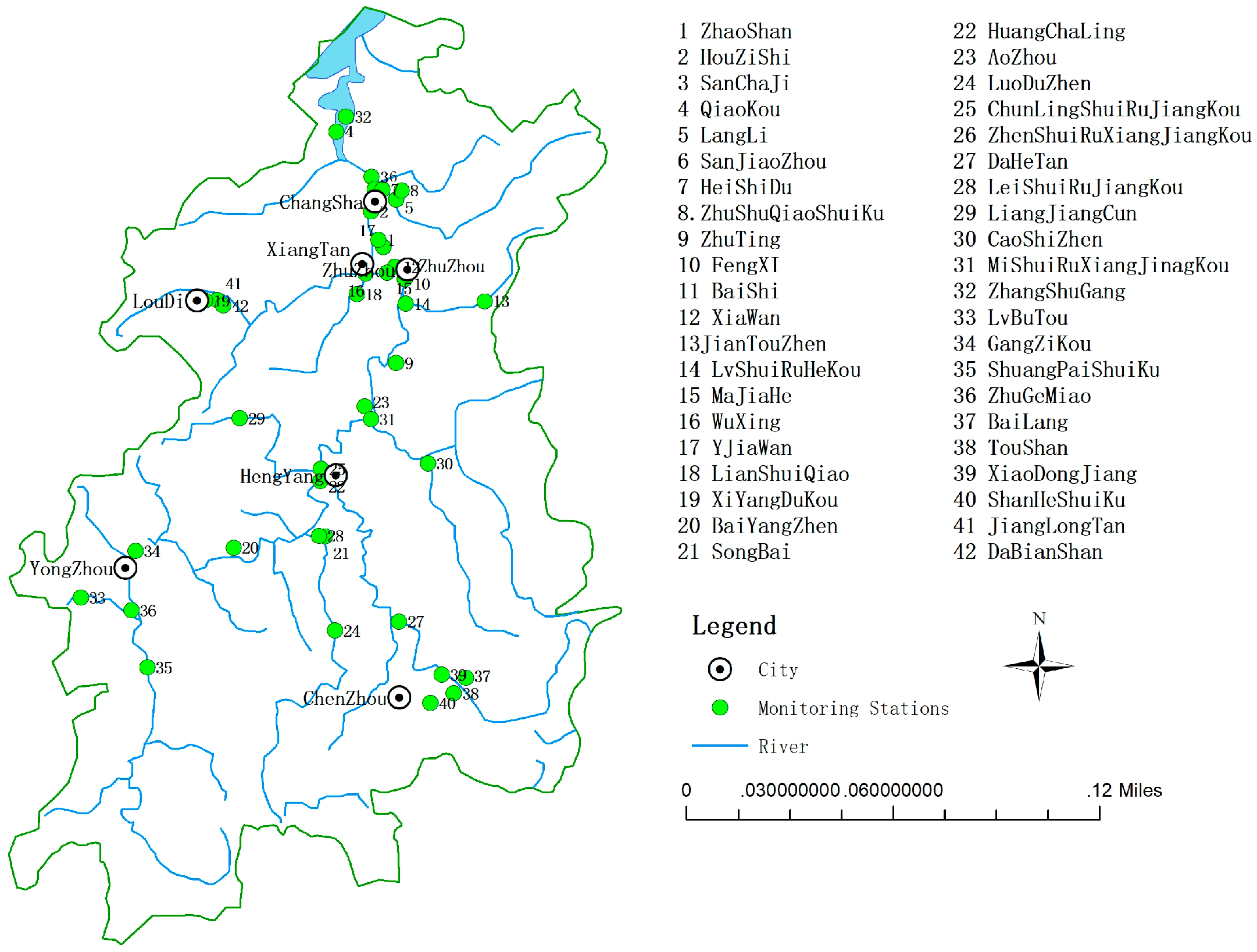
2.1. Study Site
2.2. Data and Processing
2.3. Correlations and Multicollinearity of Variables
3. Methodology
4. Empirical Results and Discussion
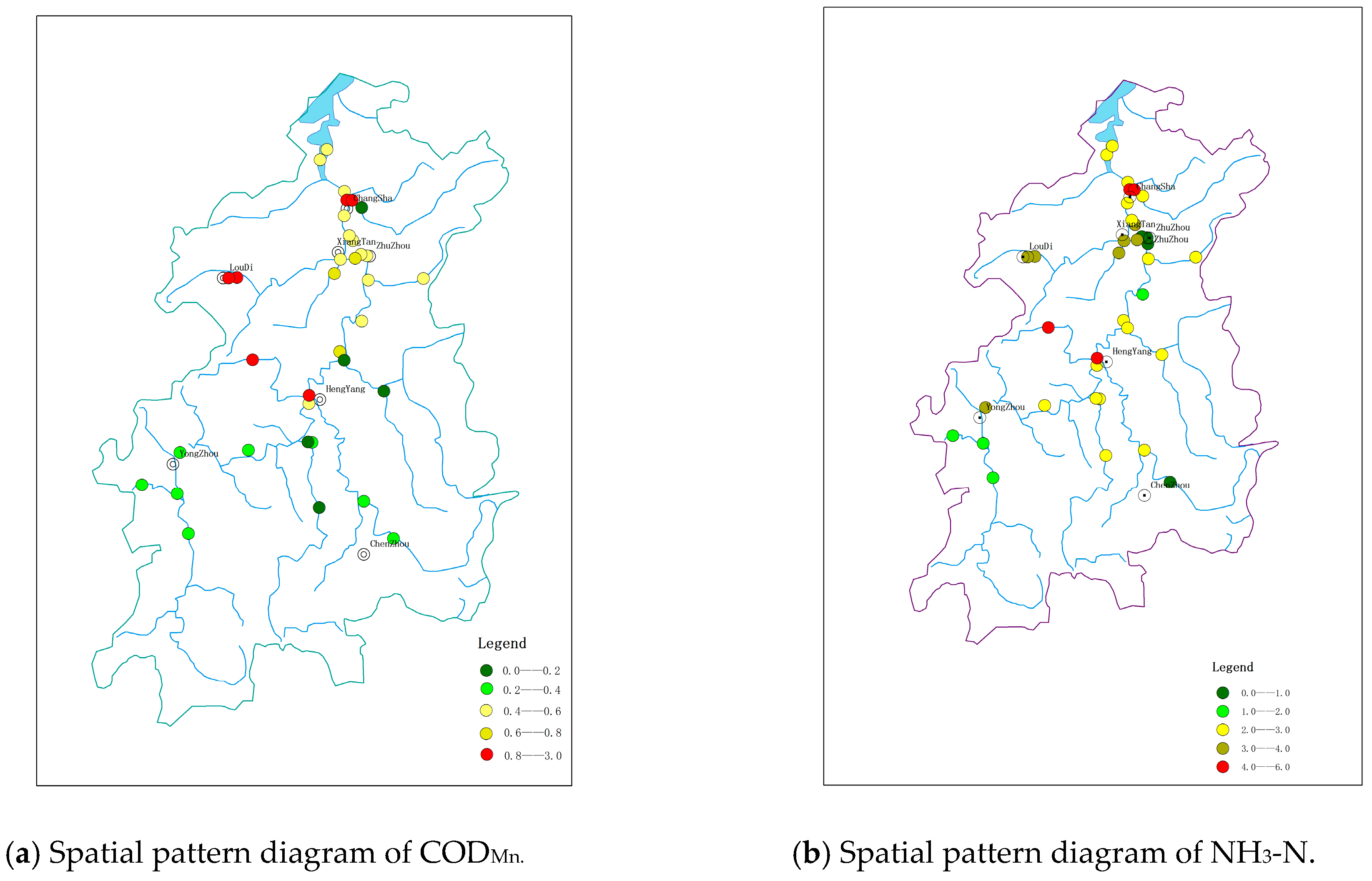
4.1. Spatial Autocorrelation for CODMn and NH3-N
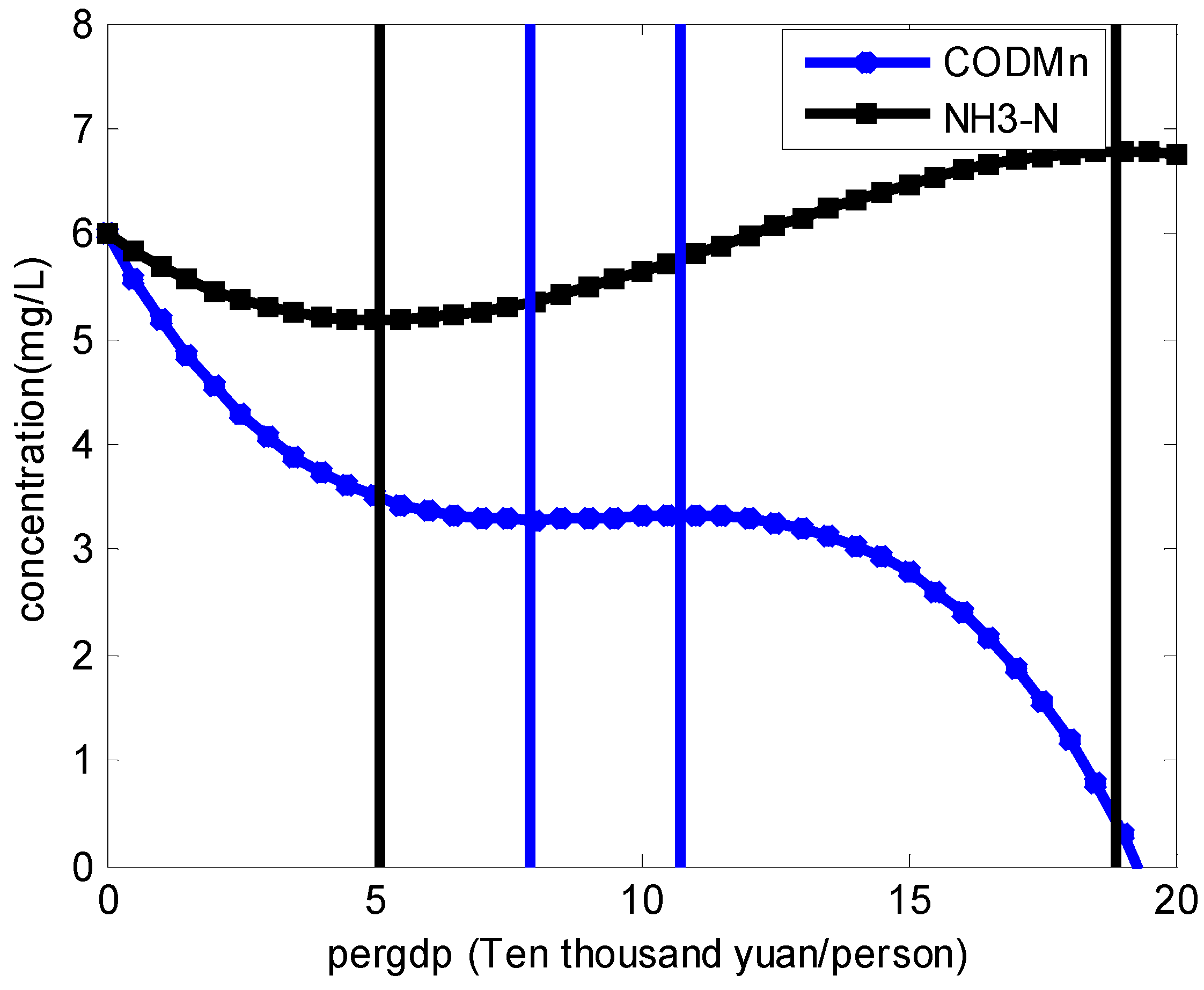
4.2. Empirical Estimation and Results
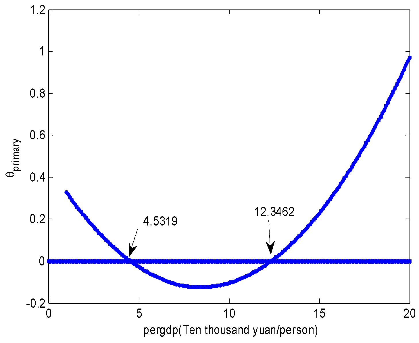
4.3. Intermediate Effect of Industrial Structure
5. Conclusions and Policy Implications
Author Contributions
Funding
Conflicts of Interest
References
- Nsubuga, F.N.; Namutebi, E.N.; Nsubuga-Ssenfuma, M. Water resources of uganda: An assessment and review. J. Water Resourc. Prot. 2014, 6, 1297–1315. [Google Scholar] [CrossRef]
- Liu, H.; Fang, C.; Zhang, X.; Wang, Z.; Bao, C.; Li, F. The effect of natural and anthropogenic factors on haze pollution in Chinese cities: A spatial econometrics approach. J. Clean. Prod. 2017, 165, 323–333. [Google Scholar] [CrossRef]
- Qian, Y.; Zheng, M.H.; Gao, L.; Zhang, B.; Liu, W.; Jiao, W.; Zhao, X.; Xiao, K. Heavy metal contamination and its environmental risk assessment in surface sediments from lake Dongting, People’s Republic of China. Bull. Environ. Contam. Toxicol. 2005, 75, 204–210. [Google Scholar] [CrossRef] [PubMed]
- Yao, Z.G.; Bao, Z.Y.; Gao, P. Environmental geochemistry of heavy metals in sediments of Dongting lake. Geochimica 2006, 35, 629–638. [Google Scholar]
- Stern, D.I.; Common, M.S. Is there an environmental kuznets curve for sulphur? J. Environ. Econ. Manag. 2001, 41, 162–178. [Google Scholar] [CrossRef]
- Copeland, B.R.; Taylor, M.S. Trade, growth, and the environment. J. Econ. Lit. 2004, 42, 7–71. [Google Scholar] [CrossRef]
- Grossman, G.M.; Krueger, B.A. Economic growth and the environment. Q. J. Econ. 1995, 110, 353–377. [Google Scholar] [CrossRef]
- Selden, T.M.; Song, D. Environmental quality and development: Is there a kuznets curve for air pollution emissions? J. Environ. Econ. Manag. 1994, 27, 147–162. [Google Scholar] [CrossRef]
- Du, Y.; Sun, X.X. Economic development and environmental quality—A case study of china prefecture-level cities. Environ. Prog. Sustain. Energy 2017, 36, 1290–1295. [Google Scholar] [CrossRef]
- Omisakin, O.A. Economic growth and environmental quality in nigeria: Does environmental kuznets curve hypothesis hold? Soc. Sci. Electr. Publ. 2009, 1, 14–18. [Google Scholar]
- Panayotou, T. Empirical Tests and Policy Analysis of Environmental Degradation at Different Stages of Economic Development; International Labour Organization: Geneva, Switzerland, 1993; pp. 2927–2978. [Google Scholar]
- Cavlovic, T.A.; Baker, K.H.; Berrens, R.P.; Gawande, K. A meta-analysis of environmental kuznets curve studies. Agric. Resour. Econ. Rev. 2000, 29, 32–42. [Google Scholar] [CrossRef]
- Galeotti, M.; Manera, M.; Lanza, A. On the Robustness of Robustness Checks of the Environmental Kuznets Curve; Pergamon Press: Oxford, UK, 2008. [Google Scholar]
- Ulucak, R.; Bilgili, F. A reinvestigation of ekc model by ecological footprint measurement for high, middle and low income countries. J. Clean. Prod. 2018, 188, 144–157. [Google Scholar] [CrossRef]
- Ahmed, K. Environmental kuznets curve and pakistan: An empirical analysis. Procedia Econ. Financ. 2012, 1, 4–12. [Google Scholar] [CrossRef]
- Apergis, N.; Ozturk, I. Testing environmental kuznets curve hypothesis in Asian countries. Ecol. Indic. 2015, 52, 16–22. [Google Scholar] [CrossRef]
- Ozturk, I.; Acaravci, A. The long-run and causal analysis of energy, growth, openness and financial development on carbon emissions in Turkey. Energy Econ. 2013, 36, 262–267. [Google Scholar] [CrossRef]
- Farhani, S.; Ozturk, I. Causal relationship between CO2 emissions, real gdp, energy consumption, financial development, trade openness, and urbanization in Tunisia. Environ. Sci. Pollut. Res. 2015, 22, 15663–15676. [Google Scholar] [CrossRef] [PubMed]
- Friedl, B.; Getzner, M. Determinants of CO2 emissions in a small open economy. Ecol. Econ. 2003, 45, 133–148. [Google Scholar] [CrossRef]
- Ge, X.; Zhou, Z.; Zhou, Y.; Ye, X.; Liu, S. A spatial panel data analysis of economic growth, urbanization, and nox emissions in China. Int. J. Environ. Res. Public Health 2018, 15, 725. [Google Scholar] [CrossRef] [PubMed]
- Moomaw, W.R.; Unruh, G.C. Are environmental kuznets curves misleading us? The case of CO2 emissions. Environ. Dev. Econ. 2001, 2, 451–463. [Google Scholar] [CrossRef]
- Governance, D.K. Institutions and the environment-income relationship: A cross-country study. Environ. Dev. Econ. 2009, 11, 705–723. [Google Scholar]
- Jaunky, V.C. The CO2, emissions-income nexus: Evidence from rich countries. Energy Policy 2011, 39, 1228–1240. [Google Scholar] [CrossRef]
- Onafowora, O.A.; Owoye, O. Bounds testing approach to analysis of the environment kuznets curve hypothesis. Energy Econ. 2014, 44, 47–62. [Google Scholar] [CrossRef]
- Lantz, V.; Feng, Q. Assessing income, population, and technology impacts on CO2, emissions in Canada: Where’s the ekc? Ecol. Econ. 2006, 57, 229–238. [Google Scholar] [CrossRef]
- Chowdhury, R.R.; Moran, E.F. Turning the curve: A critical review of kuznets approaches. Appl. Geogr. 2012, 32, 3–11. [Google Scholar] [CrossRef]
- Wang, Z.X.; Hao, P.; Yao, P.Y. Non-linear relationship between economic growth and CO2 emissions in China: An empirical study based on panel smooth transition regression models. Int. J. Environ. Res. Public Health 2017, 14, 1568. [Google Scholar] [CrossRef] [PubMed]
- Kühn, I. Incorporating spatial autocorrelation may invert observed patterns. Divers. Distrib. 2010, 12, 66–69. [Google Scholar] [CrossRef]
- Anselin, L. Spacestat Tutorial: A Workbook for Using Spacestat in the Analysis of Spatial Data; National Center for Geographic Information and Analysis; University of California: Santa Barbara, CA, USA, 1992. [Google Scholar]
- Poon, J.P.; Casas, I.; He, C. The impact of energy, transport, and trade on air pollution in China. Eurasian Geogr. Econ. 2006, 47, 568–584. [Google Scholar] [CrossRef]
- Anselin, L. The maximum likelihood approach to spatial process models. In Spatial Econometrics: Methods and Models; Kluwer Academic: Boston, MA, USA; London, UK, 1988; pp. 57–59. [Google Scholar]
- Tang, D.; Xu, H.; Yang, Y. Mutual influence of energy consumption and foreign direct investment on haze pollution in China: A spatial econometric approach. Pol. J. Environ. Stud. 2018, 27, 1743–1752. [Google Scholar] [CrossRef]
- Xu, X.; Wang, Y. Study on spatial spillover effects of logistics industry development for economic growth in the Yangtze River delta city cluster based on spatial durbin model. Int. J. Environ. Res. Public Health 2017, 14, 1508. [Google Scholar] [CrossRef] [PubMed]
- Su, S.; Xiao, R.; Xu, X.; Zhang, Z.; Mi, X.; Wu, J. Multi-scale spatial determinants of dissolved oxygen and nutrients in Qiantang River, China. Reg. Environ. Chang. 2013, 13, 77–89. [Google Scholar] [CrossRef]
- Chang, H. Spatial analysis of water quality trends in the Han river basin, South Korea. Water Res. 2008, 42, 3285–3304. [Google Scholar] [CrossRef] [PubMed]
- Chen, N.W.; Wang, L.J.; Liu, H.; Wu, J.Z.; Liu, T. A spatio-temporal correlation analysis of water quality and economic growth in the Jiulong River basin. J. Ecol. Rural Environ. 2012, 28, 19–25. [Google Scholar]
- Yang, X.; Jin, W. Gis-based spatial regression and prediction of water quality in river networks: A case study in Iowa. J. Environ. Manag. 2010, 91, 1943–1951. [Google Scholar] [CrossRef] [PubMed]
- Jordan, B.R. The environmental kuznets curve: Preliminary meta-analysis of published studies, 1995–2010. In Dans Workshop on Original Policy Research; Georgia Tech-School of Public Policy: Atlanta, GA, USA, 2010. [Google Scholar]
- Paolo Miglietta, P.; De Leo, F.; Toma, P. Environmental kuznets curve and the water footprint: An empirical analysis. Water Environ. J. 2017, 31, 20–30. [Google Scholar] [CrossRef]
- Shen, Z.; Wenjiang, D.; Licheng, Z.; Xibao, C. Geochemical characteristics of heavy metals in the Xiangjiang River, China. Hydrobiologia 1989, 176, 253–262. [Google Scholar] [CrossRef]
- Zhang, Q.; Li, Z.; Zeng, G.; Li, J.; Fang, Y.; Yuan, Q.; Wang, Y.; Ye, F. Assessment of surface water quality using multivariate statistical techniques in red soil hilly region: A case study of Xiangjiang watershed, China. Environ. Monit. Assess. 2009, 152, 123–131. [Google Scholar] [CrossRef] [PubMed]
- Dong, W.; Zhang, L.; Zhang, S. The research on the distribution and forms of heavy metals in the Xiangjiang River sediments. Chin. Geogr. Sci. 1992, 2, 42–55. [Google Scholar] [CrossRef]
- Alvarez, S.; Asci, S.; Vorotnikova, E. Valuing the potential benefits of water quality improvements in watersheds affected by non-point source pollution. Water 2016, 8, 112. [Google Scholar] [CrossRef]
- Asare, F.; Palamuleni, L.G.; Ruhiiga, T. Land use change assessment and water quality of ephemeral ponds for irrigation in the North West province, South Africa. Int. J. Environ. Res. Public Health 2018, 15, 1175. [Google Scholar] [CrossRef] [PubMed]
- Cheng, P.; Meng, F.; Wang, Y.; Zhang, L.; Yang, Q.; Jiang, M. The impacts of land use patterns on water quality in a trans-boundary river basin in northeast China based on eco-functional regionalization. Int. J. Environ. Res. Public Health 2018, 15, 1872. [Google Scholar] [CrossRef] [PubMed]
- Jiang, B.F.; Sun, W.L. Assessment of heavy metal pollution in sediments from Xiangjiang River (China) using sequential extraction and lead isotope analysis. J. Cent. South Univ. 2014, 21, 2349–2358. [Google Scholar] [CrossRef]
- Xiao, Q.; Gao, Y.; Hu, D.; Tan, H.; Wang, T. Assessment of the interactions between economic growth and industrial wastewater discharges using co-integration analysis: A case study for China’s Hunan province. Int. J. Environ. Res. Public Health 2011, 8, 2937–2950. [Google Scholar] [CrossRef] [PubMed]
- Kang, Y.Q.; Zhao, T.; Yang, Y.Y. Environmental kuznets curve for CO2 emissions in China: A spatial panel data approach. Ecol. Indic. 2016, 63, 231–239. [Google Scholar] [CrossRef]
- Maddison, D. Environmental kuznets curves: A spatial econometric approach. J. Environ. Econ. Manag. 2006, 51, 218–230. [Google Scholar] [CrossRef]
- Abreu, M.; De Groot, H.; Florax, R. Space and growth: A survey of empirical evidence and methods. Reg. Et Dev. 2004, 21, 13–44. [Google Scholar] [CrossRef]
- Madariaga, N.; Poncet, S. Fdi in Chinese cities: Spillovers and impact on growth. World Econ. 2007, 30, 837–862. [Google Scholar] [CrossRef]
- Elhorst, J.P. Dynamic spatial panels: Models, methods, and inferences. J. Geogr. Syst. 2012, 14, 5–28. [Google Scholar] [CrossRef]
- Anselin, L.; Bera, A. Spatial Dependence in Linear Regression Models with an Introduction to Spatial Econometrics; Marcel Dekker: New York, NY, USA, 1998. [Google Scholar]
- James LeSage, R.K.P. Introduction to Spatial Econometrics; Chapman and Hall/CRC: Boca Raton, FL, USA, 2009. [Google Scholar]
- Elhorst, J.P. Spatial Econometrics: From Cross-Sectional Data to Spatial Panels; Springer: Heidelberg, Germany; New York, NY, USA; Dordrecht, The Netherlands; London, UK, 2014. [Google Scholar]
- Judd, C.M.; Kenny, D.A. Process analysis: Estimating mediation in treatment evaluations. Eval. Rev. 1981, 5, 602–619. [Google Scholar] [CrossRef]
- Reuben, M.; Baron, D.A.K. The moderator-mediator variable distinction in social psychological research: Conceptual, strategic, and statistical considerations. J. Pers. Soc. Psychol. 1986, 51, 1173–1182. [Google Scholar]
- MacKinnon, D.P.; Lockwood, C.M.; Hoffman, J.M.; West, S.G.; Sheets, V. A comparison of methods to test mediation and other intervening variable effects. Psychol. Methods 2002, 7, 83–104. [Google Scholar] [CrossRef] [PubMed]
- Kroes, J.; Subramanian, R.; Subramanyam, R. Operational compliance levers, environmental performance, and firm performance under cap and trade regulation. Manuf. Serv. Oper. Manag. 2012, 14, 186–201. [Google Scholar] [CrossRef]
- Andrew, F.; Hayes, K.J.P. Quantifying and testing indirect effects in simple mediation models when the constituent paths are nonlinear. Multivar. Behav. Res. 2010, 45, 627–660. [Google Scholar]


| Variables | Unit | Sample Size | Mean | Maximum | Minimun | Std.Dev |
|---|---|---|---|---|---|---|
| CODMn | mg/L | 286 | 2.706307 | 8.27 | 0.25 | 1.112028 |
| NH3-N | mg/L | 286 | 0.5549968 | 4.17 | 0.028 | 0.6375492 |
| Pergdp | 10,000 yuan/person | 286 | 3.230058 | 15.19642 | 0.5712453 | 2.394778 |
| primary | % | 286 | 0.132208 | 0.387262 | 0.000218 | 0.104902 |
| indus | % | 286 | 0.398297 | 0.833231 | 0.075346 | 0.156605 |
| pop | 10,000 people/km2 | 286 | 0.134713 | 1.268224 | 0.009488 | 0.222809 |
| ur | % | 286 | 59.85635 | 100 | 18.51 | 26.1837 |
| precipitation | millimeter | 286 | 1368.753 | 2151 | 804 | 253.0147 |
| Variables | VIF | CODMn | NH3-N | Pergdp | Primary | Indus | Pop | Precipitation |
|---|---|---|---|---|---|---|---|---|
| CODMn | 1.07 | 1 | ||||||
| NH3-N | 1.77 | 0.58 *** | 1 | |||||
| Pergdp | 4.93 | 0.11 * | 0.44 *** | 1 | ||||
| Primary | 2.71 | −0.06 | −0.32 *** | −0.74 *** | 1 | |||
| Indus | 1.53 | −0.21 *** | −0.38 *** | −0.06 | −0.22 *** | 1 | ||
| Pop | 3.64 | 0.28 *** | 0.58 *** | 0.79 *** | −0.52 ** | −0.35 *** | 1 | |
| Precipitation | 1.05 | −0.19 *** | −0.07 | 0.16 *** | −0.12 ** | 0.08 | 0.06 | 1 |
| Variables | 2005 | 2006 | 2007 | 2008 | 2009 | 2010 | 2011 | 2012 | 2013 | 2014 | 2015 |
|---|---|---|---|---|---|---|---|---|---|---|---|
| CODMn | 0.454 | 0.336 | 0.115 | 0.178 | 0.305 | 0.062 | 0.068 | 0.193 | 0.169 | 0.258 | 0.408 |
| NH3-N | 0.647 | 0.573 | 0.565 | 0.569 | 0.633 | 0.639 | 0.338 | 0.567 | 0.355 | 0.632 | 0.871 |
| Variables | CODMn | ||||
|---|---|---|---|---|---|
| OLS | SAR | SEM | SDM | ||
| X | X × W | ||||
| Pergdp | −0.769125 ** (−2.33) | −0.814879 *** (−2.67) | −0.8491968 *** (−2.78) | −0.8627394 *** (−2.56) | 1.586722 *** (3.07) |
| Pergdp2 | 0.0568525 (1.43) | 0.0632209 * (1.72) | 0.0629587 * (1.72) | 0.0906988 ** (2.13) | −0.1469894 ** (−2.18) |
| Pergdp3 | −0.0017309 (−1.13) | −0.0019929 (−1.40) | −0.0018965 (−1.36) | −0.0031909 ** (−1.96) | 0.0047774 * (1.73) |
| primary | −7.307696 *** (−3.34) | −7.089124 *** (−3.52) | −7.416741 ** (3.66) | −6.726415 *** (−3.43) | −4.344041 (−1.49) |
| indus | −2.161912 * (−1.86) | −1.775304 (−1.61) | −1.842487 * (1.69) | −2.326853 ** (−2.07) | −5.136943 *** (−2.56) |
| pop | −2.429998 (−1.38) | −2.338575 (−1.45) | −2.133634 (−1.31) | −2.405921 (−1.45) | 0.3432917 (−0.12) |
| pre | −0.0002118 (−0.90) | −0.0002282 (−1.06) | −0.0001922 (−0.85) | −0.0000604 ** (−2.11) | −0.0001505 (0.26) |
| λ | 0.095021 (1.40) | 0.1135916 (1.52) | 0.1003935 * (1.91) | ||
| Log likelihood | −237.9421 | −237.2963 | −236.7877 | −222.8622 | |
| Lagrange Multiplier (LM) spatial lag | 3.5722 * | ||||
| LM spatial error | 4.3314 ** | ||||
| Robust LM spatial lag | 0.2122 | ||||
| Robust LM spatial error | 0.8078 | ||||
| Durbin–Watson | 1.6843 | 1.7390 | 1.6887 | 1.7900 | |
| Wald Test | 30.2044 *** | 30.8764 *** | |||
| LR Test | 28.8703 *** | 27.8688 *** | |||
| Hausman test | 27.9928 ** | ||||
| Spatial fixed effects | YES | YES | YES | YES | |
| Time fixed effects | YES | YES | YES | YES | |
| R2 | 0.0563 | 0.0604 | 0.0445 | 0.153 | |
| Variables | NH3-N | ||||
|---|---|---|---|---|---|
| OLS | SAR | SEM | SDM | ||
| X | X × W | ||||
| Pergdp | −0.2304252 * (−1.75) | −0.3599694 *** (−3.06) | −0.2796854 ** (−2.40) | −0.3831458 *** (−2.90) | 0.5121585 ** (−2.52) |
| Pergdp2 | 0.0225424 (1.42) | 0.0395953 *** (2.79) | 0.0279102 * (1.95) | 0.04656 *** (2.83) | −0.0602376 ** (−2.26) |
| Pergdp3 | −0.0002884 * (−0.44) | −0.0010476 * (−1.90) | −0.0006139 (−1.14) | −0.0012895 ** (−2.02) | 0.0022042 ** (−2.02) |
| primary | 0.8327864 (0.90) | 1.190792 (1.53) | 0.7400716 (0.91) | 1.028606 (1.33) | −2.10261 * (−1.87) |
| indus | 0.0973589 (0.20) | 0.4293576 (1.04) | 0.121705 (0.29) | 0.6328895 (1.46) | 0.1612411 (0.21) |
| pop | −5.441929 *** (−7.28) | −5.197749 *** (−8.32) | −4.009296 *** (−6.22) | −4.974618 *** (−7.59) | 1.229716 (−1.12) |
| pre | −0.0002017 ** (−2.02) | −0.0001833 ** (−2.20) | 0.0002131 ** (−2.16) | −0.0002387 (−1.10) | 0.0001564 (0.67) |
| λ | 0.5099835 *** (7.96) | 0.474194 *** (5.82) | 0.4745402 *** (7.34) 44.0426 | ||
| Log-likelihood | 7.1233 | 34.2731 | 21.5694 | ||
| LM spatial lag | 32.1044 *** | ||||
| LM spatial error | 18.5332 *** | ||||
| Robust LM spatial lag | 29.1668 *** | ||||
| Robust LM spatial error | 6.6632 ** | ||||
| Durbin-Watson | 1.5847 | 1.6830 | 1.6677 | 1.6600 | |
| Wald Test | 20.0846 *** | 27.0840 ** | |||
| LR Test | 19.3777 *** | 44.6156 *** | |||
| Hausman test | 49.4105 *** | ||||
| Spatial fixed effects | YES | YES | YES | YES | |
| Time fixed effects | YES | YES | YES | YES | |
| R2 | 0.3184 | 0.1869 | 0.1911 | 0.2286 | |
| Variables | CODMn | NH3-N | ||||
|---|---|---|---|---|---|---|
| Direct Effect | Indirect Effect | Total Effect | Direct Effect | Indirect Effect | Total Effect | |
| pergdp | −0.81844 ** (−2.39) | 1.6124 *** (3.06) | 0.79401 (1.19) | −0.3247845 ** (−2.36) | 0.518729 ** (1.88) | 0.19339 (0.54) |
| pergdp2 | 0.08473 ** (1.97) | −0.14809 ** (−2.14) | −0.0633 (−0.73) | 0.0395103 *** (2.28) | −0.06006 * (−1.65) | −0.02055 (−0.44) |
| pergdp3 | −0.002987 * (−1.79) | 0.004793 * (1.68) | 0.00118 (0.49) | −0.0012895 ** (−1.49) | 0.0023856 (−1.58) | 0.001367 (0.70) |
| primary | −6.7732 *** (−3.57) | −5.2055 * (−1.76) | −11.988 *** (−3.33) | 0.8134952 (1.08) | −2.45148 (−1.61) | −1.637988 (−0.85) |
| indus | −2.41538 ** (−2.22) | −5.4209 *** (−2.57) | −7.8363 *** (−3.20) | 0.6585608 (1.52) | 0.56817 (0.51) | 1.2267 (0.91) |
| pop | −2.4034 (−1.69) | −0.56609 (−0.19) | −2.9695 (−0.78) | −4.841386 *** (−6.93) | −0.58244 (−0.37) | −5.4238 *** (−2.67) |
| pre | −0.000578 (−0.10) | 0.0001696 (0.29) | −0.0001118 (0.44) | −0.0002219 * (−1.88) | 0.000111 (0.64) | −0.000111 (−0.85) |
| Variables | CODMn | NH3-N |
|---|---|---|
| pergdp | −0.6344118 *** (−2.59) | −0.4388021 *** (−3.64) |
| pergdp2 | 0.0404943 * (1.831) | 0.0547024 *** (3.71) |
| pergdp3 | −0.009982 * (−1.89) | −0.00160061 *** (−2.82) |
| Pop | −2.542371 (−1.47) | −5.144074 *** (−7.82) |
| pre | −0.0002308 (−0.25) | −0.0001765 (−0.83) |
| 0.171587 *** (2.77) | 0.461027 *** (5.76) | |
| Spatial fixed effects | Yes | Yes |
| Time fixed effects | Yes | Yes |
| Log-likelihood | −234.0258 | 40.6721 |
| R2 | 0.0803 | 0.1857 |
| Variables | Primary | Indus |
|---|---|---|
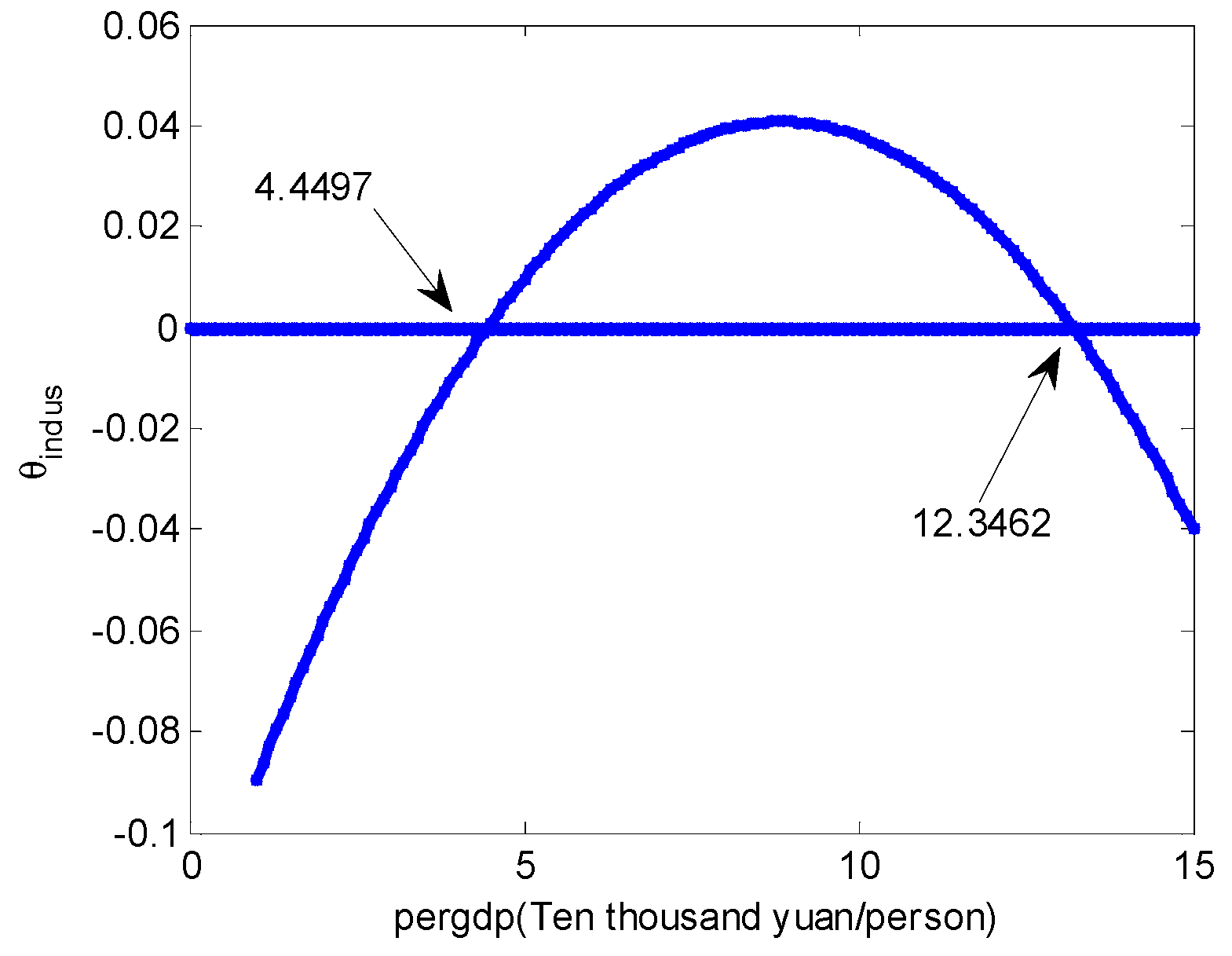
| pergdp | −0.0716853 *** (−7.8) | 0.0516433 *** (3.02) |
| pergdp2 | 0.0102196 *** (9) | −0.0077573 *** (−3.77) |
| pergdp3 | −0.0004045 *** (−9.21) | 0.0002928 *** (3.69) |
| Pop | −0.03464 (0.68) | −0.0969328 (−1.07) |
| pre | −8.14 × 10⁻⁶ (0.5) | 0.0000677 ** (2.30) |
| 0.1769211 * (1.67) | 0.1155647 (0.64) | |
| Spatial fixed effects | YES | YES |
| Time fixed effects | YES | YES |
| Log-likelihood | 763.3026 | 600.1801 |
| R2 | 0.6333 | 0.4397 |
© 2018 by the authors. Licensee MDPI, Basel, Switzerland. This article is an open access article distributed under the terms and conditions of the Creative Commons Attribution (CC BY) license (http://creativecommons.org/licenses/by/4.0/).
Share and Cite
Chen, X.; Yi, G.; Liu, J.; Liu, X.; Chen, Y. Evaluating Economic Growth, Industrial Structure, and Water Quality of the Xiangjiang River Basin in China Based on a Spatial Econometric Approach. Int. J. Environ. Res. Public Health 2018, 15, 2095. https://0-doi-org.brum.beds.ac.uk/10.3390/ijerph15102095
Chen X, Yi G, Liu J, Liu X, Chen Y. Evaluating Economic Growth, Industrial Structure, and Water Quality of the Xiangjiang River Basin in China Based on a Spatial Econometric Approach. International Journal of Environmental Research and Public Health. 2018; 15(10):2095. https://0-doi-org.brum.beds.ac.uk/10.3390/ijerph15102095
Chicago/Turabian StyleChen, Xiaohong, Guodong Yi, Jia Liu, Xiang Liu, and Yang Chen. 2018. "Evaluating Economic Growth, Industrial Structure, and Water Quality of the Xiangjiang River Basin in China Based on a Spatial Econometric Approach" International Journal of Environmental Research and Public Health 15, no. 10: 2095. https://0-doi-org.brum.beds.ac.uk/10.3390/ijerph15102095