Effects of Internal Partitions on Flow Field and Air Contaminant Distribution under Different Ventilation Modes


Abstract
:1. Introduction
2. Validation of the CFD Model
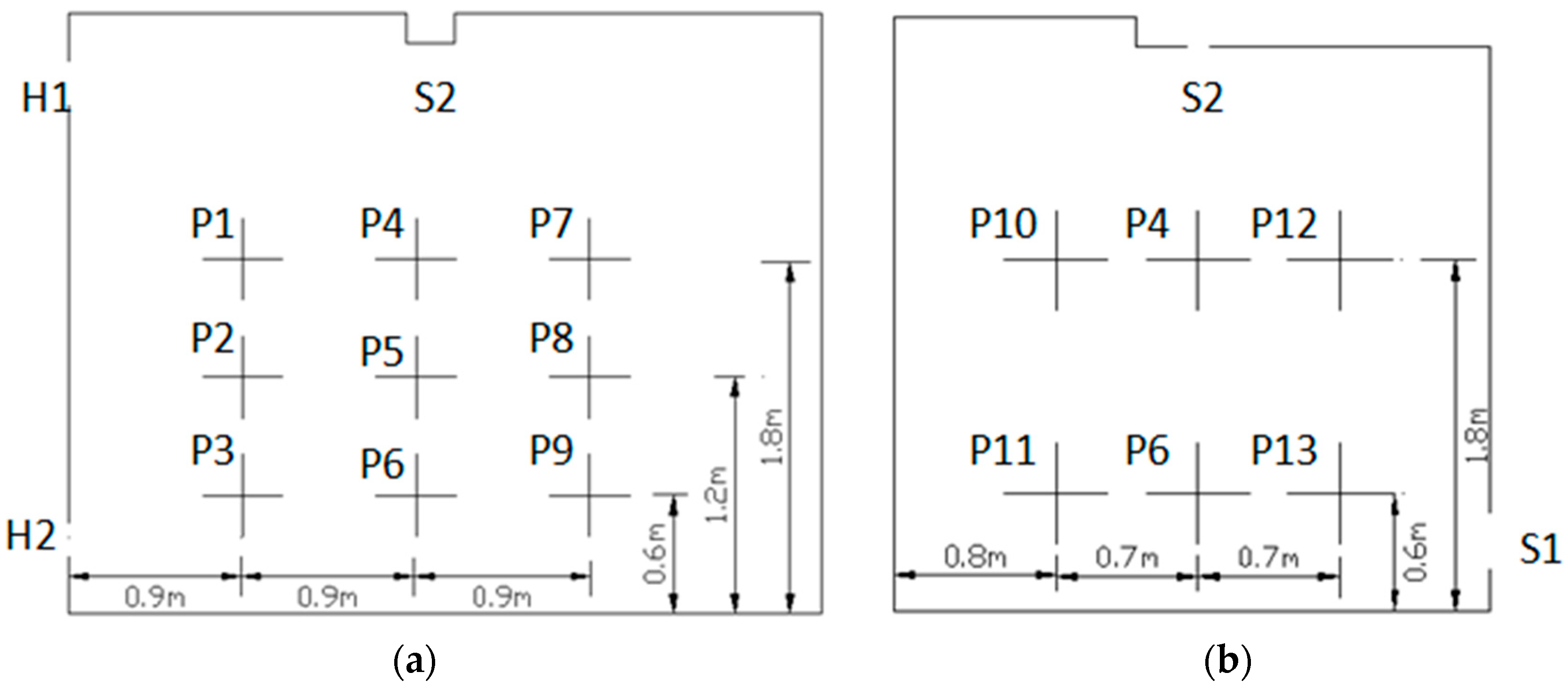
2.1. Model Test
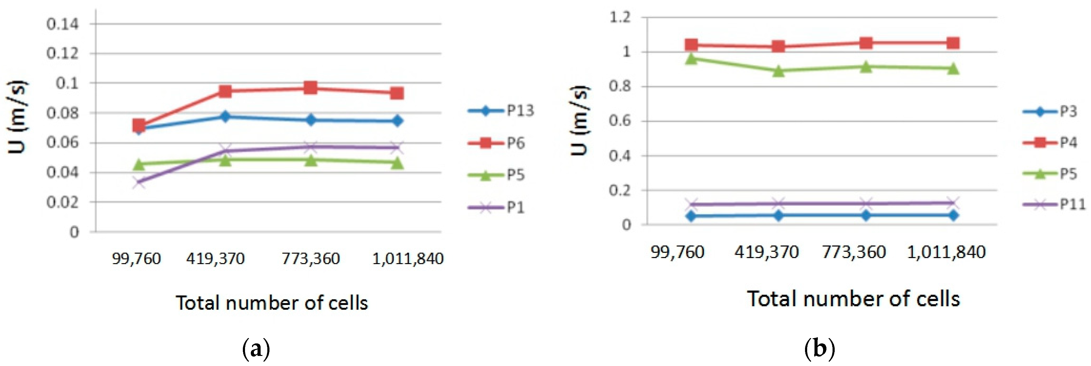
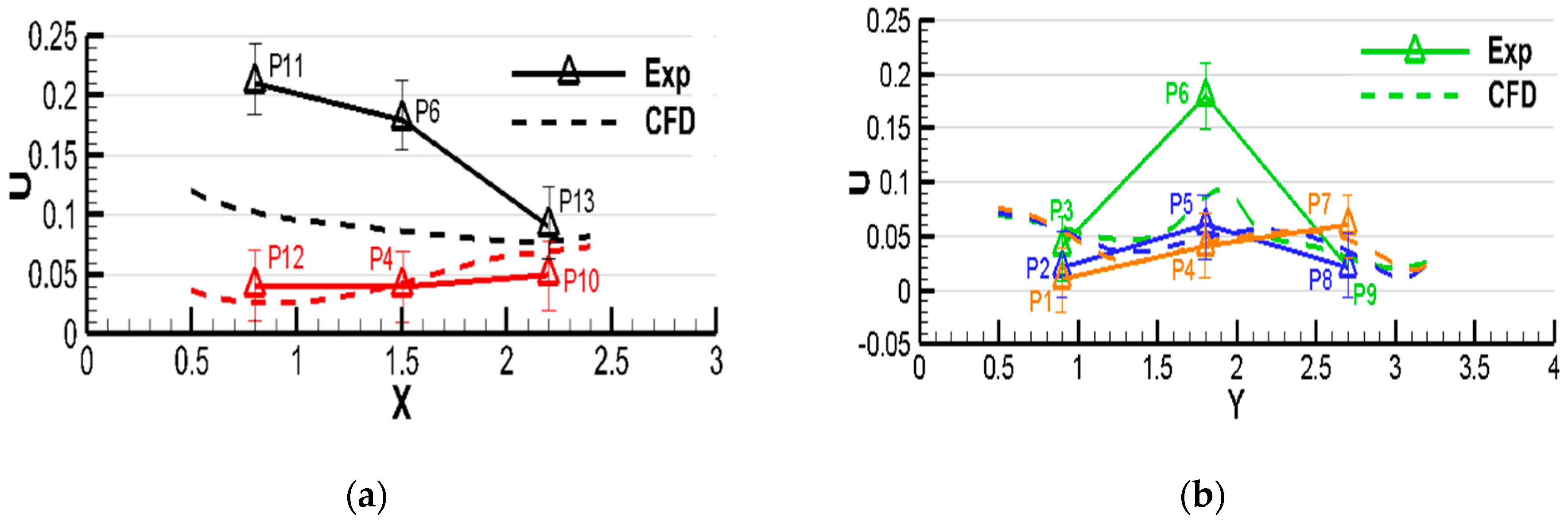
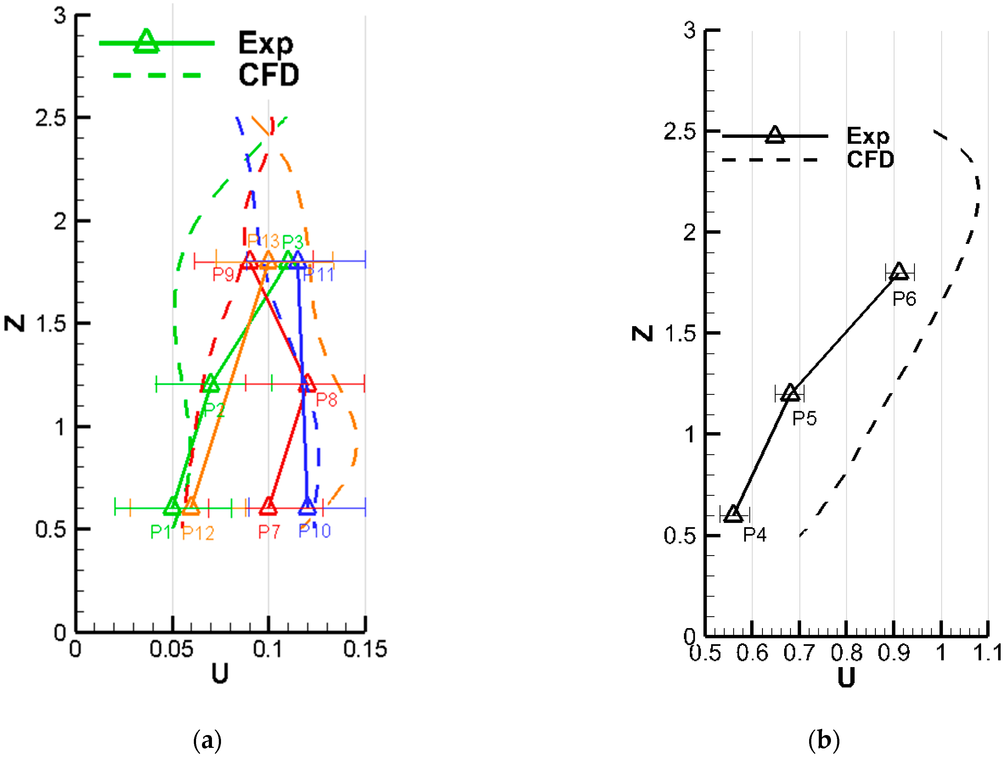
2.2. Comparisons between Simulations and Measurements
3. Case Studies
3.1. Model I Setup
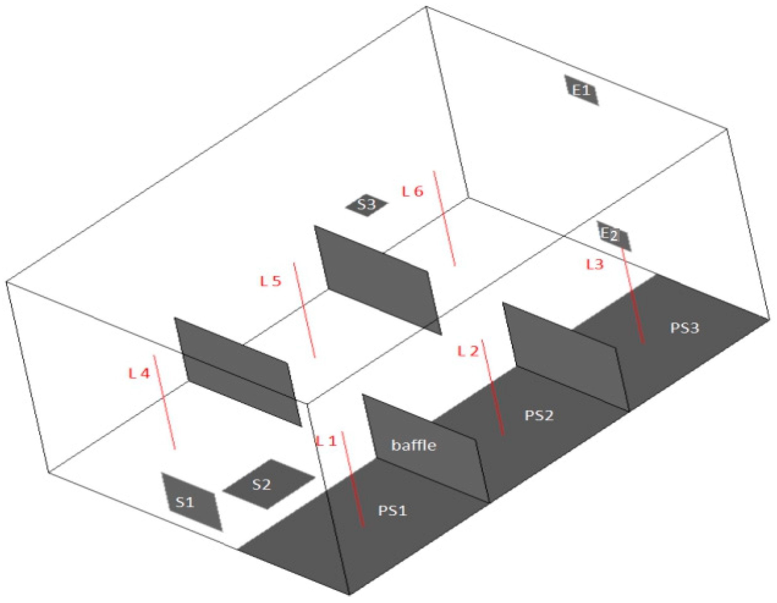
3.2. Model II Setup
4. Simulation Results and Analysis
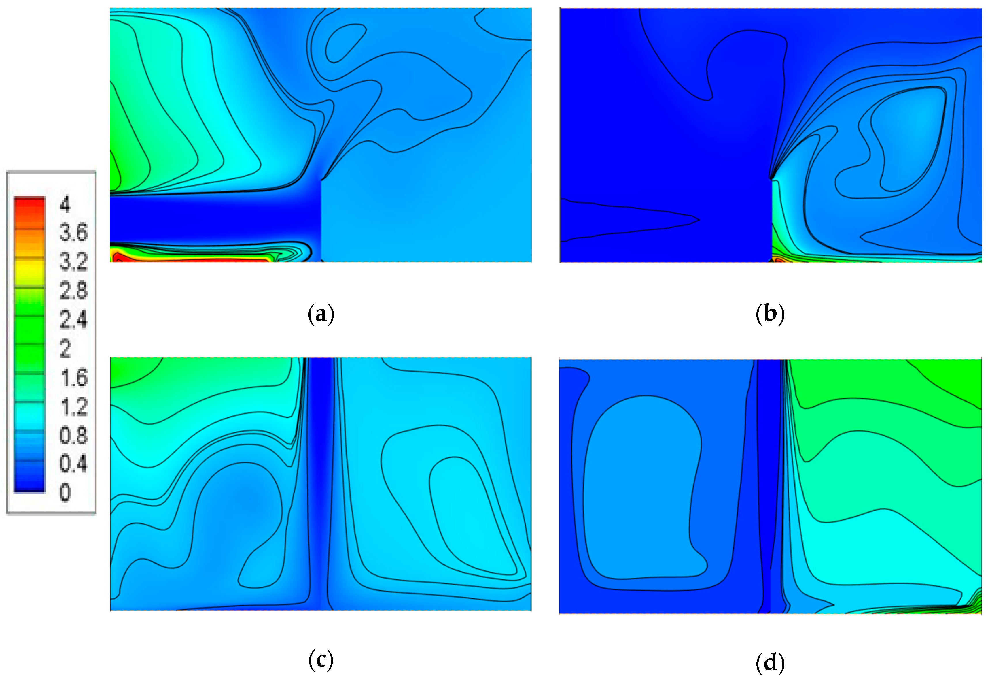
4.1. Airflow Patterns in Model I
4.2. Pollution Concentration Distributions in Model I
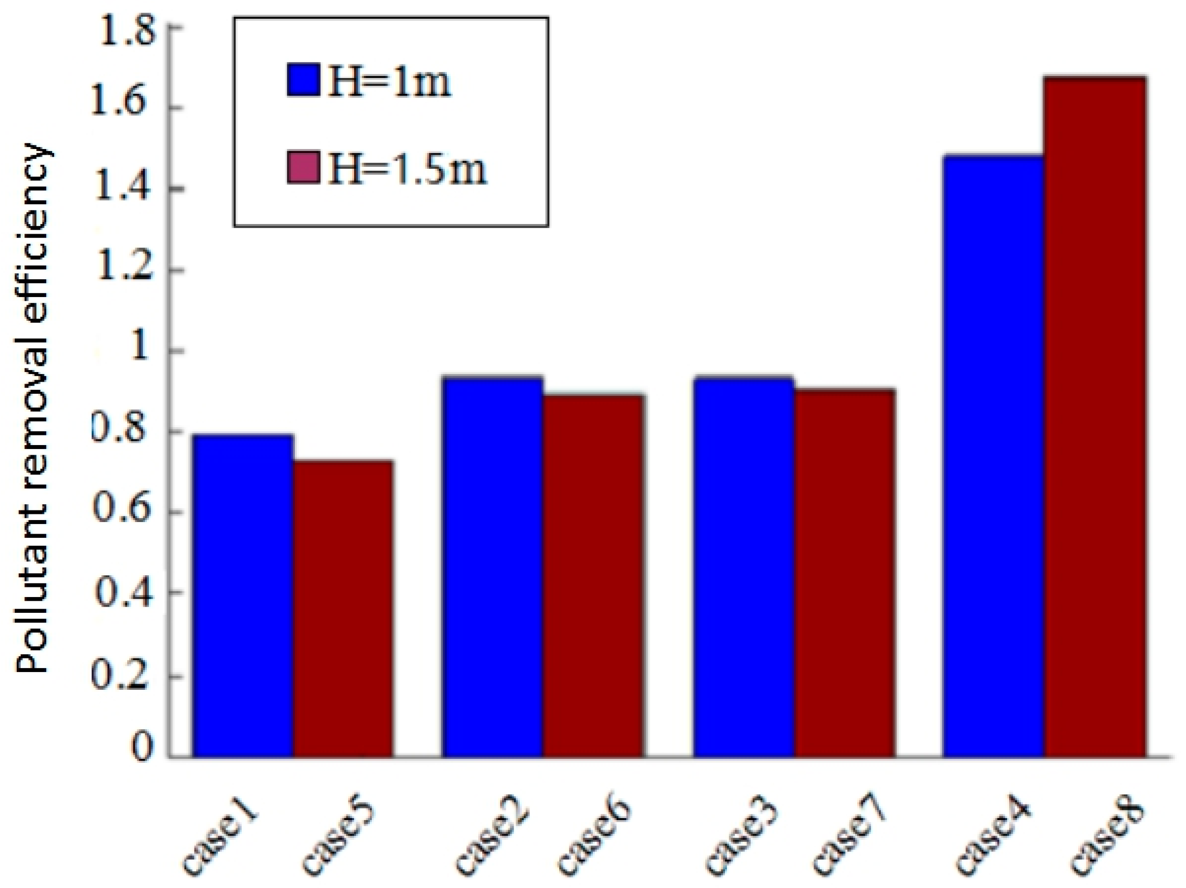
4.3. Pollution Removal Efficiency in Model I
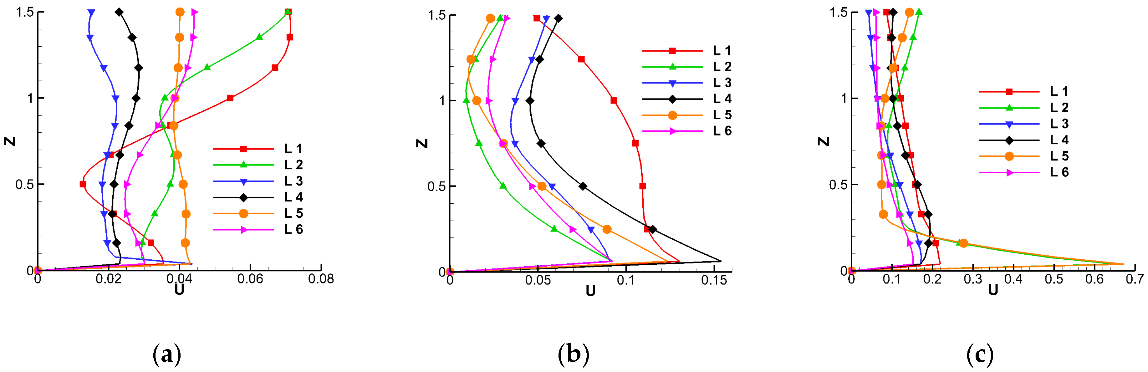
4.4. Velocity Distributions along Vertical Lines in Model II
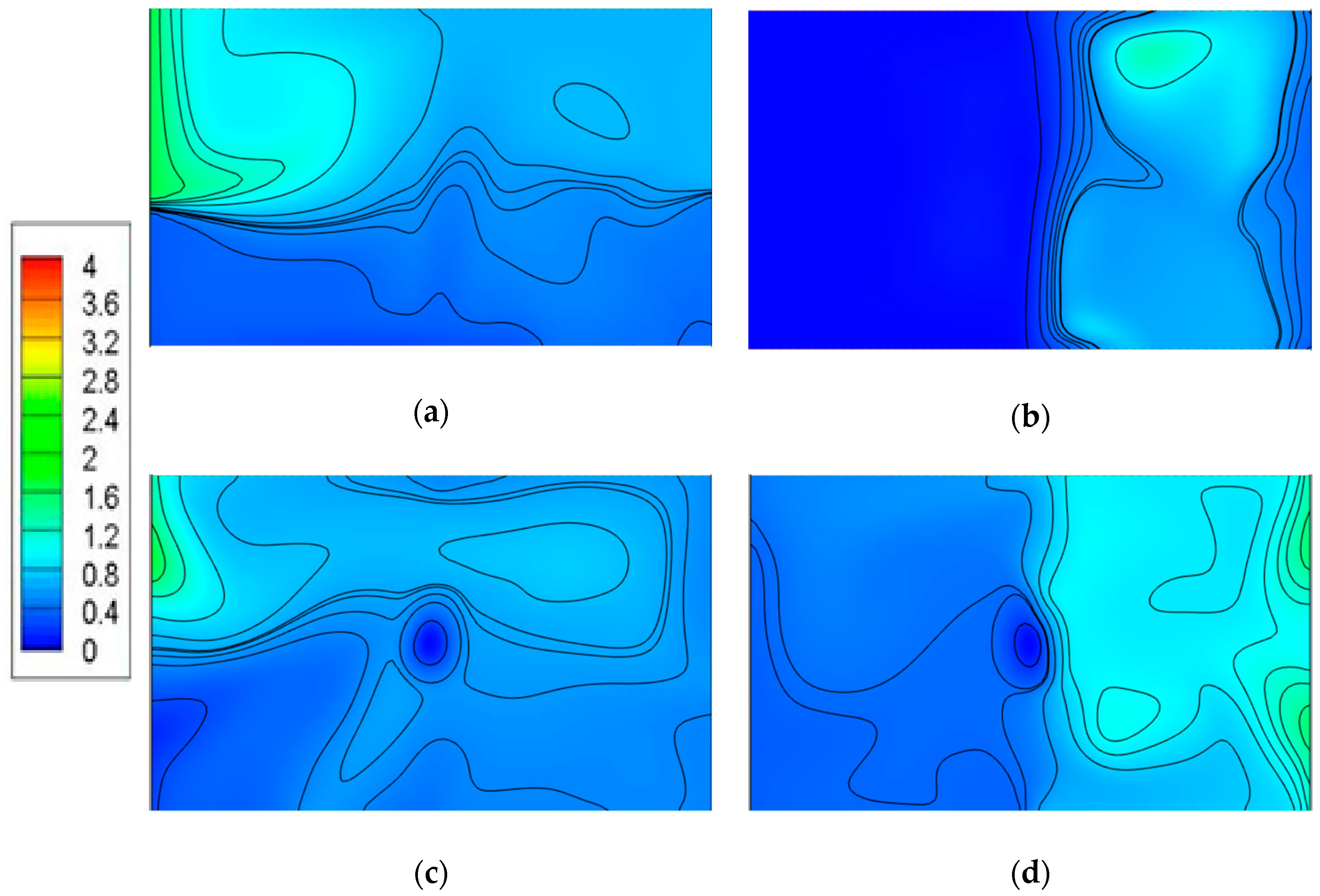
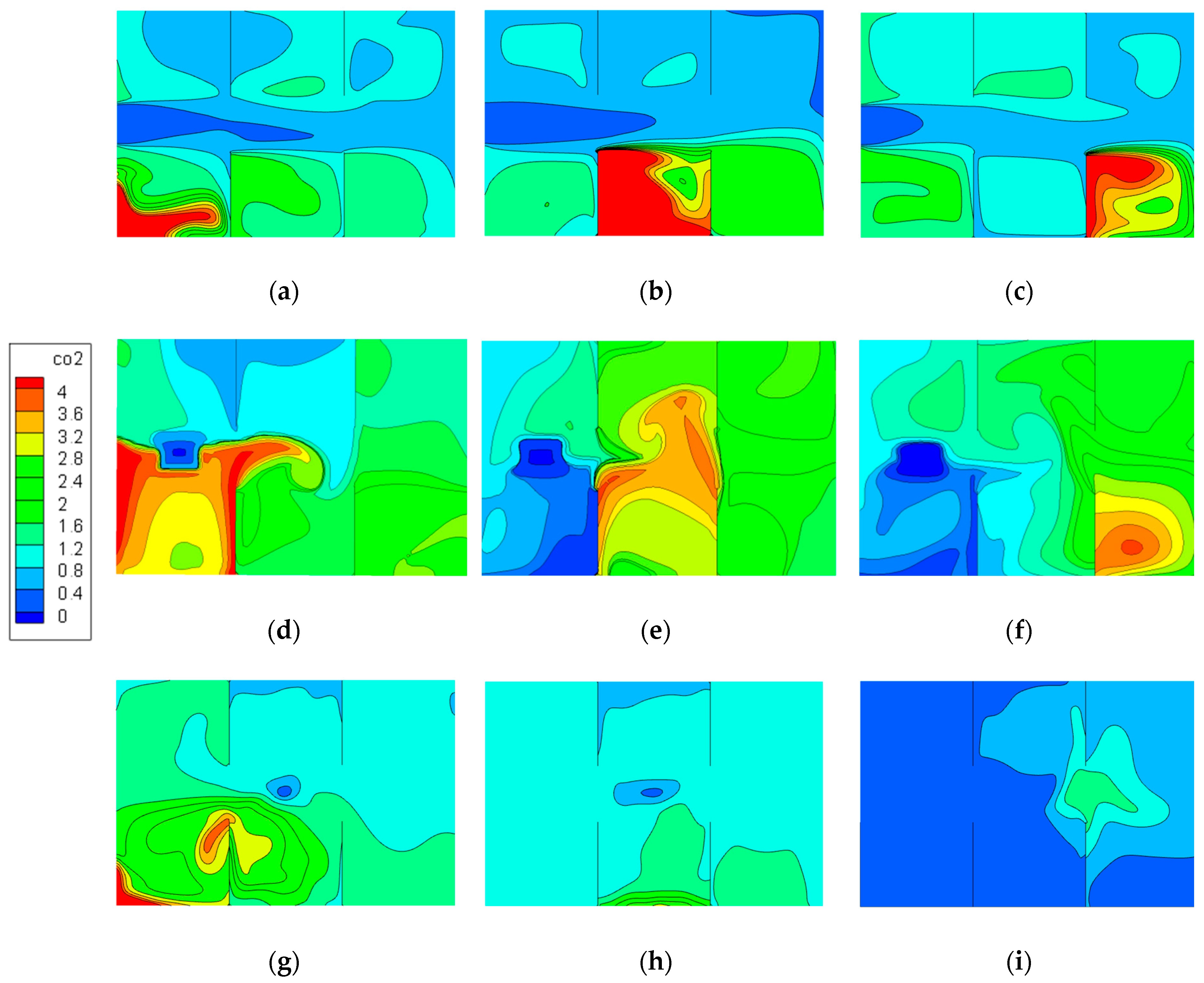
4.5. Pollutant Concentration Distributions in Model II
5. Discussion
6. Conclusions
Author Contributions
Acknowledgments
Conflicts of Interest
References
- Wang, J.N.; Cao, S.R.; Li, Z.; Li, S.M. Human exposure to carbon monoxide and inhalable particulate in Beijing, China. Biomed. Environ. Sci. 1988, 1, 5–12. [Google Scholar] [PubMed]
- Spengler, J.D.; Samet, J.M.; Mccarthy, J.F. Indoor Air Quality Handbook; McGraw-Hill Companies: New York, NY, USA, 2001. [Google Scholar]
- Wallner, P.; Munoz, U.; Tappler, P.; Wanka, A.; Kundi, M.; Shelton, J.F.; Hutter, H.P. Indoor environmental quality in mechanically ventilated, energy-efficient buildings vs. conventional buildings. Int. J. Environ. Res. Public Health 2015, 12, 14132–14147. [Google Scholar] [CrossRef] [PubMed]
- Liu, X.P.; Niu, J.L.; Perino, M.; Heiselberg, P. Numerical simulation of inter-flat air cross-contamination under the condition of single-sided natural ventilation. J. Build. Perform. Simul. 2008, 1, 133–147. [Google Scholar] [CrossRef]
- Liu, X.P.; Niu, J.L.; Kwok, K.C.S. Evaluation of RANS turbulence models for simulating wind-induced mean; pressures and dispersions around a complex-shaped high-rise building. Build. Simul. 2013, 6, 151–164. [Google Scholar] [CrossRef]
- Vornanen-Winqvist, C.; Salonen, H.; Järvi, K.; Andersson, M.A.; Mikkola, R.; Marik, T.; Kredics, L.; Kurnitski, J. Effects of ventilation improvement on measured and perceived indoor air quality in a school building with a hybrid ventilation system. Int. J. Environ. Res. Public Health 2018, 15, 1414. [Google Scholar] [CrossRef] [PubMed]
- Yang, J.; Li, X.; Zhao, B. Prediction of transient contaminant dispersion and ventilation performance using the concept of accessibility. Energy Build. 2004, 36, 293–299. [Google Scholar] [CrossRef]
- Li, X.; Chen, J. Evolution of contaminant distribution at steady airflow field with an arbitrary initial condition in ventilated space. Atmos. Environ. 2008, 42, 6775–6784. [Google Scholar] [CrossRef]
- Zhao, B.; Wu, J. Numerical Investigation of Particle Diffusion in a Clean Room. Indoor Built Environ. 2005, 14, 469–479. [Google Scholar] [CrossRef]
- Yang, X.; Chen, Q. A coupled airflow and source/sink model for simulating indoor VOC exposures. Indoor Air 2010, 11, 257–269. [Google Scholar] [CrossRef]
- Murakami, S.; Kato, S.; Chikamoto, T.; Laurence, D.; Blay, D. New low-Reynolds-number k-ε, model including damping effect due to buoyancy in a stratified flow field. Int. J. Heat Mass Transf. 1996, 39, 3483–3496. [Google Scholar] [CrossRef]
- Patton, A.P.; Calderon, L.; Xiong, Y.; Wang, Z.; Senick, J.; Sorensen Allacci, M.; Plotnik, D.; Wener, R.; Andrews, C.J.; Krogmann, U.; et al. Airborne particulate matter in two multi-family green buildings: Concentrations and effect of ventilation and occupant behavior. Int. J. Environ. Res. Public Health 2016, 13, 144. [Google Scholar] [CrossRef] [PubMed]
- Cao, Q.; He, X.G. Cross ventilation and room partitions: Wind tunnel experiments on indoor airflow distribution. ASHRAE Trans. 1994, 100, 208–219. [Google Scholar]
- Chu, C.R.; Chiang, B.F. Wind-driven cross ventilation with internal obstacles. Energy Build. 2013, 67, 201–209. [Google Scholar] [CrossRef]
- Bauman, F.S. Air Movement, Ventilation, and Comfort in Partitioned Office Space. ASHRAE Trans. 1992, 98, 756–780. [Google Scholar]
- Lee, H.; Awbi, H.B. Effect of internal partitioning on indoor air quality of rooms with mixing ventilation—Basic study. Build. Environ. 2004, 39, 127–141. [Google Scholar] [CrossRef]
- Lee, H.; Awbi, H.B. Effect of internal partitioning on room air quality with mixing ventilation—Statistical analysis. Renew. Energy 2004, 29, 1721–1732. [Google Scholar] [CrossRef]
- Fontanini, A.; Vaidya, U.; Ganapathysubramanian, B. A stochastic approach to modeling the dynamics of natural ventilation systems. Energy Build. 2013, 63, 87–97. [Google Scholar] [CrossRef]
- Fontanini, A.; Olsen, M.G.; Ganapathysubramanian, B. Thermal comparison between ceiling diffusers and fabric ductwork diffusers for green buildings. Energy Build. 2011, 43, 2973–2987. [Google Scholar] [CrossRef] [Green Version]
- Noh, K.-C.; Jang, J.-S.; Oh, M.-D. Thermal comfort and indoor air quality in the lecture room with 4-way cassette air-conditioner and mixing ventilation system. Build. Environ. 2007, 42, 689–698. [Google Scholar] [CrossRef]
- Noh, K.-C.; Han, C.-W.; Oh, M.-D. Effect of the airflow rate of a ceiling type air-conditioner on ventilation effectiveness in a lecture room. Int. J. Refrig. 2008, 31, 180–188. [Google Scholar] [CrossRef]
- Method of Testing for Room Air Diffusion (ASHRAE). ANSI/ASHRAE Standard 113-1990, Method of Testing for Room Air Diffusion; American Society of Heating, Refrigerating, and Air-Conditioning Engineers, Inc.: Atlanta, GA, USA, 1990. [Google Scholar]
- Chung, K.C.; Hsu, S.P. Effect of ventilation pattern on room air and contaminant distribution. Build. Environ. 2001, 36, 989–998. [Google Scholar] [CrossRef]
- Nakshatrala, K.B.; Mudunuru, M.K.; Valocchi, A.J. A numerical framework for diffusion-controlled bimolecular-reactive systems to enforce maximum principles and the non-negative constraint. J. Comput. Phys. 2013, 253, 278–307. [Google Scholar] [CrossRef] [Green Version]
- Mudunuru, M.K.; Nakshatrala, K.B. On enforcing maximum principles and achieving element-wise species balance for advection-diffusion-reaction equations under the finite element method. J. Comput. Phys. 2016, 305, 448–493. [Google Scholar] [CrossRef]
- Mazumdar, S.; Yin, G.; Guity, A.; Marmion, P.; Gulick, B.; Chen, Q. Impact of Moving Objects on Contaminant Concentration Distributions in an Inpatient Ward with Displacement Ventilation. Sci. Technol. Built Environ. 2010, 16, 545–563. [Google Scholar]


| Test Item | Instrument Name | Measurement Range | Accuracy | Sample Interval |
|---|---|---|---|---|
| Air velocity | Alnor Balometer Capture Hood EBT731 | Air volume: 42–4250 m3/h Air velocity: 0.125–40 m/s | 0.1 m3/h | 10–600 s |
| Indoor velocity field/temperature field | Swema 03+ omnidirectional anemometer | Air temperature: +10 to +40 °C Air velocity: 0.05–5.00 m/s | 0.03 m/s/3% | 0.2 s |
| Name | Room | Supply Inlet S1 | Supply Inlet S2 | Exhaust Outlet E1 | Exhaust Outlet E2 | Baffle | Pollution Source PS1 | Pollution Source PS2 |
|---|---|---|---|---|---|---|---|---|
| Size | 5.0 m × 3.0 m × 3.0 m | 0.7 m × 0.6 m | 0.3 m × 0.3 m | 0.4 m × 0.3 m | 0.4 m × 0.3 m | 3 m × 1.0 m | 2.5 m × 3.0 m | 2.5 m × 3.0 m |
| Case No. | Inlet | Outlet | Air Velocity (m/s) | Air Change Rate (times/h) | Pollution Source | Baffle Height (m) |
|---|---|---|---|---|---|---|
| Case 1 | S1 | E1 | 0.3 | 10 | PS1 | 1.0 |
| Case 2 | S1 | E1 | 0.3 | 10 | PS2 | 1.0 |
| Case 3 | S2 | E2 | 1.4 | 10 | PS1 | 1.0 |
| Case 4 | S2 | E2 | 1.4 | 10 | PS2 | 1.0 |
| Case 5 | S1 | E1 | 0.3 | 10 | PS1 | 1.5 |
| Case 6 | S1 | E1 | 0.3 | 10 | PS2 | 1.5 |
| Name | Room | Supply Inlet S1 | Supply Inlet S2 | Supply Inlet S3 | Exhaust Outlet E1 | Exhaust Outlet E2 | Baffle | Pollution Source PS1, PS2, PS3 |
|---|---|---|---|---|---|---|---|---|
| Size | 6.0 m × 4.0 m × 3.0 m | 0.7 m × 0.6 m | 0.7 m × 0.6 m | 0.3 m × 0.3 m | 0.4 m × 0.3 m | 0.4 m × 0.3 m | 1.5 m × 1 m | 2 m × 1.5 m |
| Case No. | Inlet | Outlet | Air Change Rate (times/h) | Pollution Source | Baffle Height (m) |
|---|---|---|---|---|---|
| Case 9 | S1 | E1 | 10 | PS1 | 1 |
| Case 10 | S1 | E1 | 10 | PS2 | 1 |
| Case 11 | S1 | E1 | 10 | PS3 | 1 |
| Case 12 | S2 | E1 | 10 | PS1 | 1 |
| Case 13 | S2 | E1 | 10 | PS2 | 1 |
| Case 14 | S2 | E1 | 10 | PS3 | 1 |
| Case 15 | S3 | E2 | 10 | PS1 | 1 |
| Case 16 | S3 | E2 | 10 | PS2 | 1 |
| Case 17 | S3 | E2 | 10 | PS3 | 1 |
© 2018 by the authors. Licensee MDPI, Basel, Switzerland. This article is an open access article distributed under the terms and conditions of the Creative Commons Attribution (CC BY) license (http://creativecommons.org/licenses/by/4.0/).
Share and Cite
Liu, X.; Wu, X.; Chen, L.; Zhou, R. Effects of Internal Partitions on Flow Field and Air Contaminant Distribution under Different Ventilation Modes. Int. J. Environ. Res. Public Health 2018, 15, 2603. https://0-doi-org.brum.beds.ac.uk/10.3390/ijerph15112603
Liu X, Wu X, Chen L, Zhou R. Effects of Internal Partitions on Flow Field and Air Contaminant Distribution under Different Ventilation Modes. International Journal of Environmental Research and Public Health. 2018; 15(11):2603. https://0-doi-org.brum.beds.ac.uk/10.3390/ijerph15112603
Chicago/Turabian StyleLiu, Xiaoping, Xiaojiao Wu, Linjing Chen, and Rui Zhou. 2018. "Effects of Internal Partitions on Flow Field and Air Contaminant Distribution under Different Ventilation Modes" International Journal of Environmental Research and Public Health 15, no. 11: 2603. https://0-doi-org.brum.beds.ac.uk/10.3390/ijerph15112603