A Novel Hybrid Data-Driven Model for Daily Land Surface Temperature Forecasting Using Long Short-Term Memory Neural Network Based on Ensemble Empirical Mode Decomposition

Abstract
:1. Introduction
2. Methodology Descriptions
2.1. Empirical Mode Decomposition (EMD)
2.2. Ensemble EMD (EEMD)
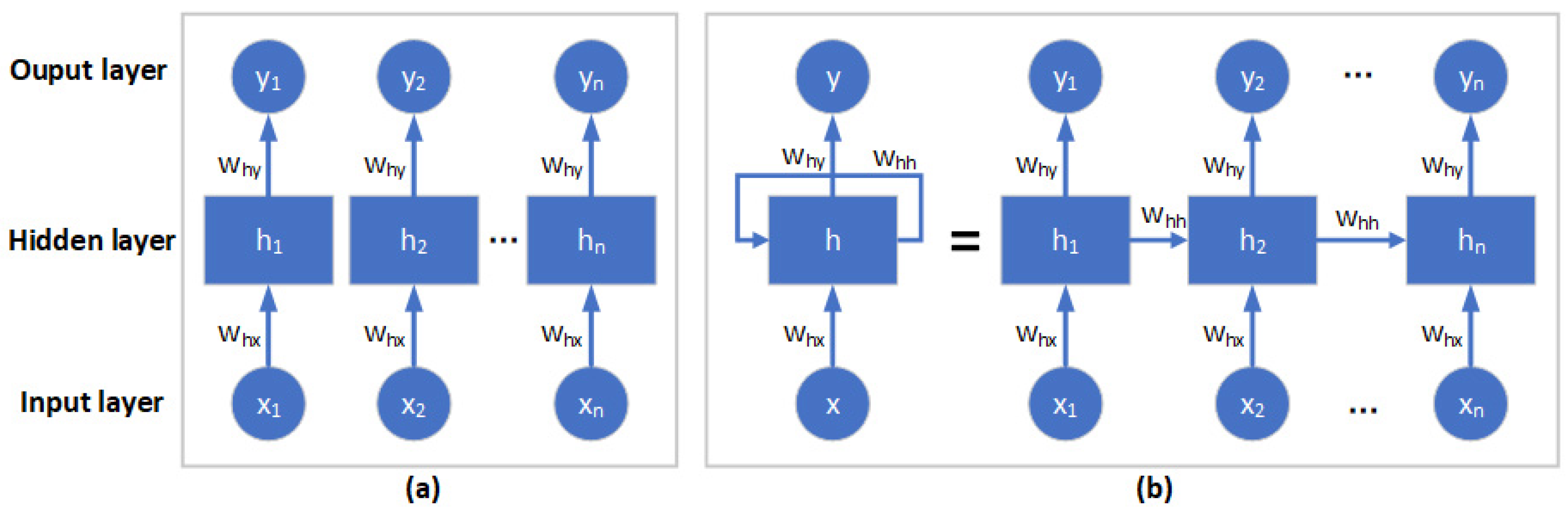
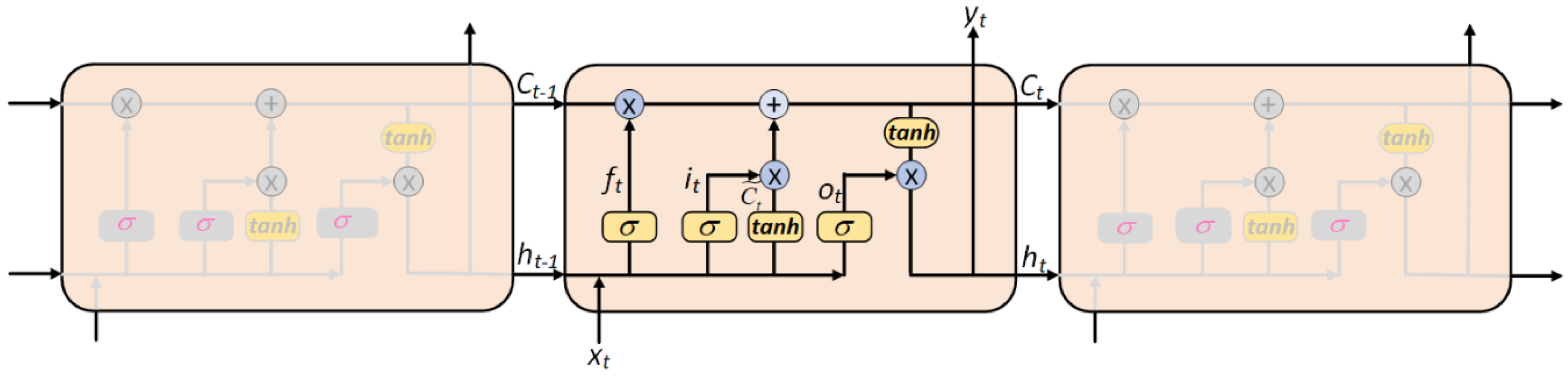
2.3. Long Short-Term Memory (LSTM) Neural Network
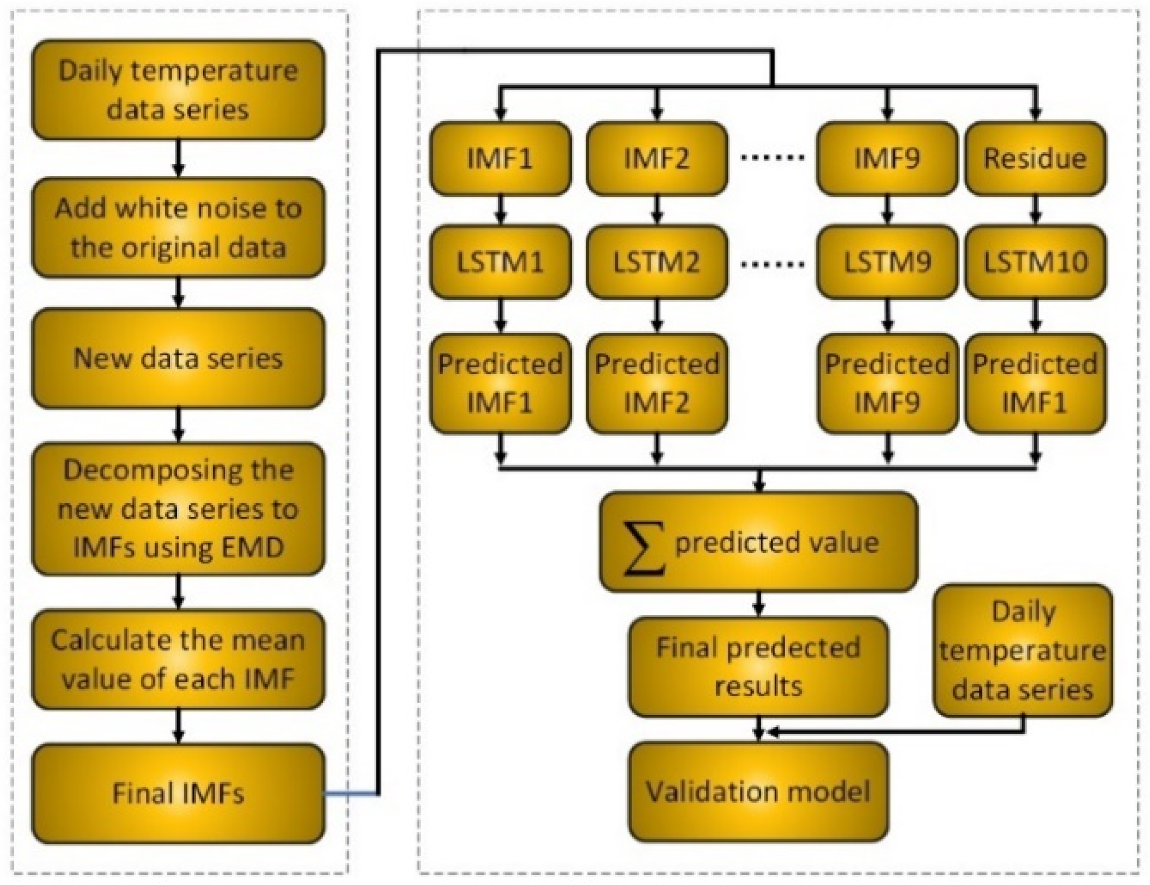
2.4. The Novel Hybrid EEMD-LSTM Data-Driven Model
3. Case Study
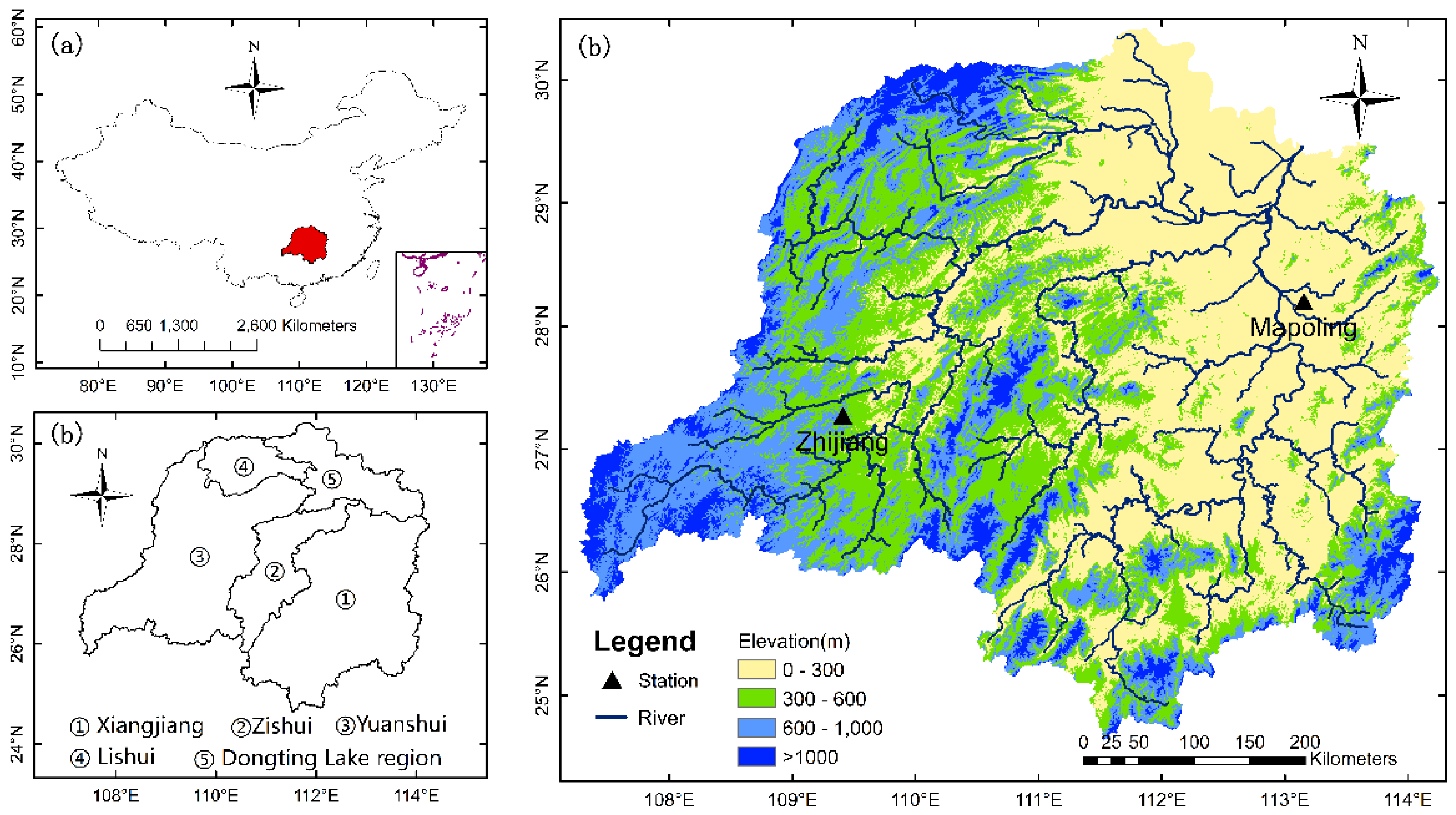
3.1. Study Area
3.2. Data Collection
3.3. Statistical Evaluation Metrics for Forecasting Performance
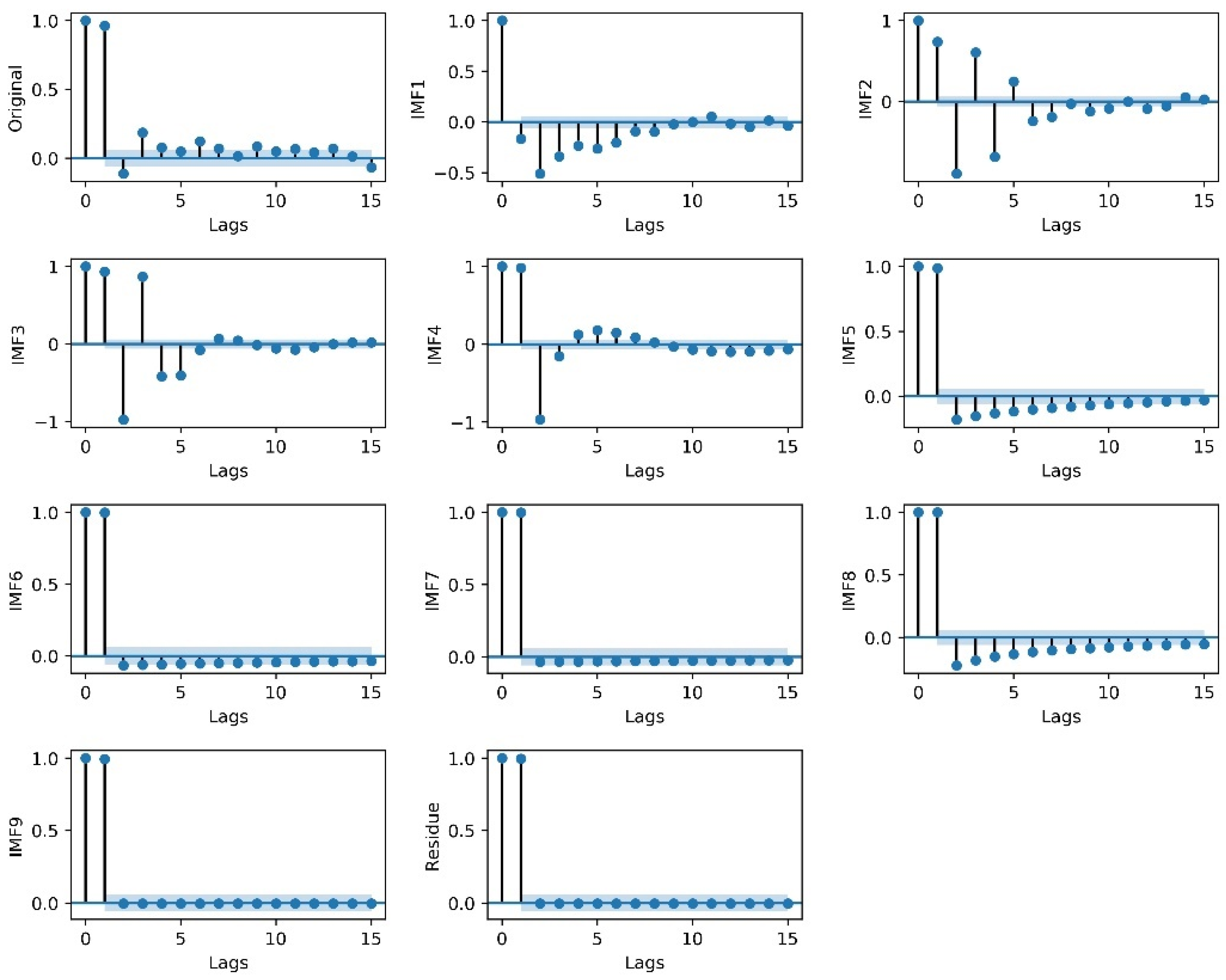
3.4. Daily LST Data Series Decomposition by EEMD
3.5. Forecasting IMFs
3.6. Performance Comparison Analysis
4. Conclusions
Author Contributions
Funding
Acknowledgments
Conflicts of Interest
Appendix A


| Series | Period | Min. | Max. | Mean | Variance | SD 1 | Skewness | Kurtosis |
|---|---|---|---|---|---|---|---|---|
| Original data set | 1 January 2014 to 31 December 2016 | −0.7 | 31.8 | 18.0538 | 63.8016 | 7.9876 | −0.2423 | −1.1268 |
| 1 January 2014 to 30 June 2016 (Training) | −0.7 | 30.85 | 17.5038 | 61.452 | 7.8391 | −0.2228 | −1.1137 | |
| 1 July 2016 to 31 December 2015 (Testing) | 3.15 | 31.8 | 20.7796 | 66.5181 | 8.1559 | −0.491 | −1.1334 | |
| IMF1 | 1 January 2014 to 31 December 2016 | −3.4876 | 3.3164 | −0.0006 | 1.0313 | 1.0155 | −0.006 | 0.5469 |
| 1 January 2014 to 30 June 2016 (Training) | −3.4876 | 3.3164 | −0.0038 | 1.0904 | 1.0442 | 0.0142 | 0.4111 | |
| 1 July 2016 to 31 December 2016 (Testing) | −2.6808 | 2.4776 | 0.0154 | 0.738 | 0.8591 | −0.1602 | 1.4322 | |
| IMF2 | 1 January 2014 to 31 December 2016 | −4.9666 | 4.6916 | −0.0137 | 1.4461 | 1.2025 | −0.0209 | 1.3251 |
| 1 January 2014 to 30 June 2016 (Training) | −4.9666 | 4.6916 | −0.0151 | 1.4498 | 1.2041 | −0.0145 | 1.3825 | |
| 1 July 2016 to 31 December 2016 (Testing) | −3.5345 | 3.7363 | −0.0067 | 1.4281 | 1.195 | −0.0533 | 1.0959 | |
| IMF3 | 1 January 2014 to 31 December 2016 | −3.9453 | 4.4972 | −0.0368 | 1.5168 | 1.2316 | 0.0842 | 0.8224 |
| 1 January 2014 to 30 June 2016 (Training) | −3.9453 | 4.4972 | −0.0552 | 1.5108 | 1.2292 | 0.0978 | 0.899 | |
| 1 July 2016 to 31 December 2016 (Testing) | −3.6699 | 3.4617 | 0.0546 | 1.5364 | 1.2395 | 0.0151 | 0.5368 | |
| IMF4 | 1 January 2014 to 31 December 2016 | −3.2607 | 3.8574 | −0.0131 | 1.0952 | 1.0465 | −0.0819 | 1.0059 |
| 1 January 2014 to 30 June 2016 (Training) | −3.2607 | 3.8574 | −0.0216 | 1.1767 | 1.0848 | −0.0533 | 0.9823 | |
| 1 July 2016 to 31 December 2016 (Testing) | −2.0462 | 1.8588 | 0.029 | 0.6889 | 0.83 | −0.2818 | −0.2253 | |
| IMF5 | 1 January 2014 to 31 December 2016 | −3.8762 | 5.271 | 0.0365 | 1.05 | 1.0247 | 0.3922 | 6.5503 |
| 1 January 2014 to 30 June 2016 (Training) | −3.8762 | 5.271 | 0.0542 | 1.1226 | 1.0595 | 0.4193 | 6.897 | |
| 1 July 2016 to 31 December 2016 (Testing) | −1.2743 | 1.1222 | −0.051 | 0.6811 | 0.8253 | −0.1313 | −1.4911 | |
| IMF6 | 1 January 2014 to 31 December 2016 | −11.189 | 11.9534 | 0.7483 | 46.884 | 6.8472 | −0.1075 | −1.3765 |
| 1 January 2014 to 30 June 2016 (Training) | −10.6116 | 10.1684 | 0.1262 | 42.3756 | 6.5097 | −0.0985 | −1.4462 | |
| 1 July 2016 to 31 December 2016 (Testing) | −11.189 | 11.9534 | 3.8314 | 57.8063 | 7.603 | −0.5543 | −1.1442 | |
| IMF7 | 1 January 2014 to 31 December 2016 | −1.6727 | 1.9026 | −0.0502 | 0.7532 | 0.8679 | 0.9044 | −0.1937 |
| 1 January 2014 to 30 June 2016 (Training) | −1.6727 | 1.9026 | 0.047 | 0.8221 | 0.9067 | 0.7038 | −0.6052 | |
| 1 July 2016 to 31 December 2016 (Testing) | −0.9499 | 0.2884 | −0.5321 | 0.1329 | 0.3645 | 0.6622 | −0.7966 | |
| IMF8 | 1 January 2014 to 31 December 2016 | −0.496 | 0.5448 | 0.0197 | 0.1395 | 0.3736 | 0.0206 | −1.5351 |
| 1 January 2014 to 30 June 2016 (Training) | −0.496 | 0.5448 | 0.0921 | 0.1335 | 0.3654 | −0.3236 | −1.362 | |
| 1 July 2016 to 31 December 2016 (Testing) | −0.4884 | −0.0747 | −0.339 | 0.0148 | 0.1216 | 0.569 | −0.9077 | |
| IMF9 | 1 January 2014 to 31 December 2016 | −0.0582 | 0.0586 | 0.0196 | 0.0012 | 0.0349 | −0.6397 | −0.8556 |
| 1 January 2014 to 30 June 2016 (Training) | −0.0582 | 0.0586 | 0.0283 | 0.0009 | 0.0306 | −1.1161 | 0.3131 | |
| 1 July 2016 to 31 December 2016 (Testing) | −0.0582 | 0.0068 | −0.0235 | 0.0004 | 0.0189 | −0.1403 | −1.1839 | |
| Residue | 1 January 2014 to 31 December 2016 | 16.2408 | 17.8054 | 17.345 | 0.2196 | 0.4686 | −0.7969 | −0.652 |
| 1 January 2014 to 30 June 2016 (Training) | 16.2408 | 17.8008 | 17.2537 | 0.2142 | 0.4628 | −0.5833 | −0.9155 | |
| 1 July 2016 to 31 December 2016 (Testing) | 17.7763 | 17.8054 | 17.798 | 0.0001 | 0.0083 | −1.1065 | −0.0229 |
References
- Abdel-Aal, R.E. Hourly temperature forecasting using abductive networks. Eng. Appl. Artif. Intell. 2004, 17, 543–556. [Google Scholar] [CrossRef]
- Salcedo-Sanz, S.; Deo, R.C.; Carro-Calvo, L.; Saavedra-Moreno, B. Monthly prediction of air temperature in Australia and New Zealand with machine learning algorithms. Theor. Appl. Climatol. 2016, 125, 13–25. [Google Scholar] [CrossRef]
- Kim, K.S.; Taylor, S.E.; Gleason, M.L.; Koehler, K.J. Model to enhance site-specific estimation of leaf wetness duration. Plant Dis. 2002, 86, 179–185. [Google Scholar] [CrossRef]
- Yao, Z.; Lou, G.; Zeng, X.; Zhao, Q. Research and Development Precision Irrigation Control System in Agricultural, Proceeding of the IEEE 2010 International Conference on Computer and Communication Technologies in Agriculture Engineering (CCTAE), Chengdu, China, 12–13 June 2010; IEEE: Chengdu, China, 2010; pp. 117–120. [Google Scholar]
- Araghi, A.; Mousavi-Baygi, M.; Adamowski, J.; Martinez, C.; van der Ploeg, M. Forecasting soil temperature based on surface air temperature using a wavelet artificial neural network. Meteorol. Appl. 2017, 24, 603–611. [Google Scholar] [CrossRef]
- Kamarianakis, Y.; Ayuso, S.V.; Rodríguez, E.C.; Velasco, M.T. Water temperature forecasting for Spanish rivers by means of nonlinear mixed models. J. Hydrol.: Reg. Stud. 2016, 5, 226–243. [Google Scholar] [CrossRef]
- Karimi, M.; Vant-Hull, B.; Nazari, R.; Mittenzwei, M.; Khanbilvardi, R. Predicting surface temperature variation in urban settings using real-time weather forecasts. Urban Clim. 2017, 20, 192–201. [Google Scholar] [CrossRef]
- Ouellet-Proulx, S.; Chimi Chiadjeu, O.; Boucher, M.-A.; St-Hilaire, A. Assimilation of water temperature and discharge data for ensemble water temperature forecasting. J. Hydrol. 2017, 554, 342–359. [Google Scholar] [CrossRef]
- Benyahya, L.; Caissie, D.; St-Hilaire, A.; Ouarda, T.B.M.J.; Bobée, B. A review of statistical water temperature models. Can. Water Resour. J. 2007, 32, 179–192. [Google Scholar] [CrossRef]
- Piccolroaz, S.; Calamita, E.; Majone, B.; Gallice, A.; Siviglia, A.; Toffolon, M. Prediction of river water temperature: A comparison between a new family of hybrid models and statistical approaches. Hydrol. Process. 2016, 30, 3901–3917. [Google Scholar] [CrossRef]
- Sahoo, G.B.; Schladow, S.G.; Reuter, J.E. Forecasting stream water temperature using regression analysis, artificial neural network, and chaotic non-linear dynamic models. J. Hydrol. 2009, 378, 325–342. [Google Scholar] [CrossRef]
- Sohrabi, M.M.; Benjankar, R.; Tonina, D.; Wenger, S.J.; Isaak, D.J. Estimation of daily stream water temperatures with a bayesian regression approach. Hydrol. Process. 2017, 31, 1719–1733. [Google Scholar] [CrossRef]
- Toffolon, M.; Piccolroaz, S. A hybrid model for river water temperature as a function of air temperature and discharge. Environ. Res. Lett. 2015, 10, 114011. [Google Scholar] [CrossRef]
- Attoue, N.; Shahrour, I.; Younes, R. Smart building: Use of the artificial neural network approach for indoor temperature forecasting. Energies 2018, 11, 395. [Google Scholar] [CrossRef]
- Deihimi, A.; Orang, O.; Showkati, H. Short-term electric load and temperature forecasting using wavelet echo state networks with neural reconstruction. Energy 2013, 57, 382–401. [Google Scholar] [CrossRef]
- Huddart, B.; Subramanian, A.; Zanna, L.; Palmer, T. Seasonal and decadal forecasts of atlantic sea surface temperatures using a linear inverse model. Clim. Dyn. 2016, 49, 1833–1845. [Google Scholar] [CrossRef]
- Khan, M.Z.K.; Sharma, A.; Mehrotra, R. Using all data to improve seasonal sea surface temperature predictions: A combination-based model forecast with unequal observation lengths. Int. J. Climatol. 2018. [Google Scholar] [CrossRef]
- Manzanas, R.; Gutiérrez, J.M.; Fernández, J.; van Meijgaard, E.; Calmanti, S.; Magariño, M.E.; Cofiño, A.S.; Herrera, S. Dynamical and statistical downscaling of seasonal temperature forecasts in Europe: Added value for user applications. Clim. Serv. 2017, 9, 44–56. [Google Scholar] [CrossRef]
- Yang, Q.; Wang, M.; Overland, J.E.; Wang, W.; Collow, T.W. Impact of model physics on seasonal forecasts of surface air temperature in the Arctic. Mon. Weather Rev. 2017, 145, 773–782. [Google Scholar] [CrossRef]
- Young, P.C. Data-based mechanistic modelling and forecasting globally averaged surface temperature. Int. J. Forecast. 2018, 34, 314–335. [Google Scholar] [CrossRef]
- Obrist, D.; Kirk, J.L.; Zhang, L.; Sunderland, E.M.; Jiskra, M.; Selin, N.E. A review of global environmental mercury processes in response to human and natural perturbations: Changes of emissions, climate, and land use. Ambio 2018, 47, 116–140. [Google Scholar] [CrossRef] [PubMed]
- Slater, L.J.; Villarini, G.; Bradley, A.A. Weighting of nmme temperature and precipitation forecasts across Europe. J. Hydrol. 2017, 552, 646–659. [Google Scholar] [CrossRef]
- Zhao, X.-H.; Chen, X. Auto regressive and ensemble empirical mode decomposition hybrid model for annual runoff forecasting. Water Resour. Manag. 2015, 29, 2913–2926. [Google Scholar] [CrossRef]
- Deo, R.C.; Sahin, M. An extreme learning machine model for the simulation of monthly mean streamflow water level in Eastern Queensland. Environ. Monit. Assess. 2016, 188, 90. [Google Scholar] [CrossRef] [PubMed]
- Deo, R.C.; Şahin, M. Application of the extreme learning machine algorithm for the prediction of monthly effective drought index in Eastern Australia. Atmos. Res. 2015, 153, 512–525. [Google Scholar] [CrossRef]
- Deo, R.C.; Tiwari, M.K.; Adamowski, J.F.; Quilty, J.M. Forecasting effective drought index using a wavelet extreme learning machine (W-elm) model. Stoch. Environ. Res. Risk A 2017, 31, 1211–1240. [Google Scholar] [CrossRef]
- Jiao, G.; Guo, T.; Ding, Y. A new hybrid forecasting approach applied to hydrological data: A case study on precipitation in northwestern China. Water 2016, 8, 367. [Google Scholar] [CrossRef]
- Luo, Y.; Chang, X.; Peng, S.; Khan, S.; Wang, W.; Zheng, Q.; Cai, X. Short-term forecasting of daily reference evapotranspiration using the hargreaves–samani model and temperature forecasts. Agric. Water Manag. 2014, 136, 42–51. [Google Scholar] [CrossRef]
- Nastos, P.T.; Paliatsos, A.G.; Koukouletsos, K.V.; Larissi, I.K.; Moustris, K.P. Artificial neural networks modeling for forecasting the maximum daily total precipitation at Athens, Greece. Atmos. Res. 2014, 144, 141–150. [Google Scholar] [CrossRef]
- Wang, W.C.; Chau, K.W.; Qiu, L.; Chen, Y.B. Improving forecasting accuracy of medium and long-term runoff using artificial neural network based on eemd decomposition. Environ. Res. 2015, 139, 46–54. [Google Scholar] [CrossRef] [PubMed]
- Zhang, X.; Zhang, Q.; Zhang, G.; Nie, Z.; Gui, Z. A hybrid model for annual runoff time series forecasting using elman neural network with ensemble empirical mode decomposition. Water 2018, 10, 416. [Google Scholar] [CrossRef]
- Balluff, S.; Bendfeld, J.; Krauter, S. Meteorological data forecast using RNN. Int. J. Grid High Perf. 2017, 9, 61–74. [Google Scholar] [CrossRef]
- Xu, S.; Niu, R. Displacement prediction of baijiabao landslide based on empirical mode decomposition and long short-term memory neural network in three gorges area, China. Comput. Geosci. 2018, 111, 87–96. [Google Scholar] [CrossRef]
- Yang, Y.T.; Dong, J.Y.; Sun, X.; Lima, E.; Mu, Q.Q.; Wang, X.H. A CFCC-LSTM model for sea surface temperature prediction. IEEE Geosci. Remote Sens. Lett. 2018, 15, 207–211. [Google Scholar] [CrossRef]
- Wei, S.; Yang, H.; Song, J.; Abbaspour, K.; Xu, Z. A wavelet-neural network hybrid modelling approach for estimating and predicting river monthly flows. Hydrol. Sci. J. 2013, 58, 374–389. [Google Scholar] [CrossRef]
- Chen, B.F.; Wang, H.D.; Chu, C.C. Wavelet and artificial neural network analyses of tide forecasting and supplement of tides around Taiwan and South China sea. Ocean Eng. 2007, 34, 2161–2175. [Google Scholar] [CrossRef]
- Nourani, V.; Alami, M.T.; Aminfar, M.H. A combined neural-wavelet model for prediction of ligvanchai watershed precipitation. Eng. Appl. Artif. Intell. 2009, 22, 466–472. [Google Scholar] [CrossRef]
- Pandey, A.S.; Singh, D.; Sinha, S.K. Intelligent hybrid wavelet models for short-term load forecasting. IEEE Trans. Power Syst. 2010, 25, 1266–1273. [Google Scholar] [CrossRef]
- Shafaei, M.; Kisi, O. Lake level forecasting using wavelet-svr, wavelet-anfis and wavelet-arma conjunction models. Water Resour. Manag. 2016, 30, 79–97. [Google Scholar] [CrossRef]
- Zhang, F.P.; Dai, H.C.; Tang, D.S. A conjunction method of wavelet transform-particle swarm optimization-support vector machine for streamflow forecasting. J. Appl. Math. 2014, 1–10. [Google Scholar] [CrossRef]
- Torrence, C.; Compo, G.P. A practical guide to wavelet analysis. Bull. Am. Meteorol. Soc. 1997, 79, 61–78. [Google Scholar] [CrossRef]
- Wu, Z.; Huang, N.E. Ensemble empirical mode decomposition: A noise-assisted data analysis method. Adv. Adapt. Data Anal. 2009, 1, 1–41. [Google Scholar] [CrossRef]
- Huang, N.E.; Shen, Z.; Long, S.R.; Wu, M.C.; Shih, H.H.; Zheng, Q.; Yen, N.C.; Tung, C.C.; Liu, H.H. The empirical mode decomposition and the hilbert spectrum for nonlinear and non-stationary time series analysis. Proc. R. Soc. A 1998, 454, 903–995. [Google Scholar] [CrossRef]
- Wang, W.-C.; Chau, K.-W.; Xu, D.-M.; Chen, X.-Y. Improving forecasting accuracy of annual runoff time series using arima based on eemd decomposition. Water Resour. Manag. 2015, 29, 2655–2675. [Google Scholar] [CrossRef]
- Zhang, N.; Lin, A.; Shang, P. Multidimensionalk-nearest neighbor model based on eemd for financial time series forecasting. Physica A 2017, 477, 161–173. [Google Scholar] [CrossRef]
- Niu, M.; Gan, K.; Sun, S.; Li, F. Application of decomposition-ensemble learning paradigm with phase space reconstruction for day-ahead PM2.5 concentration forecasting. J. Environ. Manag. 2017, 196, 110–118. [Google Scholar] [CrossRef] [PubMed]
- Huang, N.E.; Shen, Z.; Long, S.R. A new view of nonlinear water waves: The hilbert spectrum. Annu. Rev. Fluid Mech. 1999, 31, 417–457. [Google Scholar] [CrossRef]
- Giles, C.L.; Lawrence, S.; Tsoi, A.C. Noisy time series prediction using recurrent neural networks and grammatical inference. Mach. Learn. 2001, 44, 161–183. [Google Scholar] [CrossRef]
- Kan, M.S.; Tan, A.C.C.; Mathew, J. A review on prognostic techniques for non-stationary and non-linear rotating systems. Mech. Syst. Signal Proc. 2015, 62–63, 1–20. [Google Scholar] [CrossRef]
- Rius, A.; Ruisánchez, I.; Callao, M.P.; Rius, F.X. Reliability of analytical systems: Use of control charts, time series models and recurrent neural networks (RNN). Chemometr. Intell. Lab. 1998, 40, 1–18. [Google Scholar] [CrossRef]
- Schmidhuber, J. Deep learning in neural networks: An overview. Neural Netw. 2015, 61, 85–117. [Google Scholar] [CrossRef] [PubMed]
- Bengio, Y.; Simard, P.; Frasconi, P. Learning long-term dependencies with gradient descent is difficult. IEEE Trans. Neural Netw. 1994, 5, 157–166. [Google Scholar] [CrossRef] [PubMed]
- Hochreiter, S.; Schmidhuber, J. Long short-term memory. Neural Comput. 1997, 9, 1735–1780. [Google Scholar] [CrossRef] [PubMed]
- Zhang, X.; Zhang, Q.; Zhang, G.; Gui, Z. A comparison study of normalized difference water index and object-oriented classification method in river network extraction from landsat-tm imagery. In Proceedings of the IEEE 2017 2nd International Conference on Frontiers of Sensors Technologies, Shenzhen, China, 14–16 April 2017; pp. 198–2013. [Google Scholar]
- Zhang, X.; Zhang, Q.; Zhang, G.; Nie, Z.; Gui, Z. Landsat-based tow decades land cover change in Dongting Lake region. Fresen Environ. Bull. 2018, 27, 1563–1573. [Google Scholar]
- Kang, A.; Tan, Q.; Yuan, X.; Lei, X.; Yuan, Y. Short-term wind speed prediction using EEMD-LSSVM model. Adv. Meteorol. 2017, 2017, 1–22. [Google Scholar] [CrossRef]
- Google. Google Tensorflow. Available online: https://www.tensorflow.org/ (accessed on 4 September 2018).


| Series | Period | Min. | Max. | Mean | Variance | SD 1 | Skewness | Kurtosis |
|---|---|---|---|---|---|---|---|---|
| Original data set | 1 January 2014 to 31 December 2016 | −1.5 | 32.8 | 17.6599 | 67.8232 | 8.2355 | −0.2036 | −1.0706 |
| 1 January 2014 to 30 June 2016 (Training) | −1.5 | 32 | 17.0957 | 65.1861 | 8.0738 | −0.2059 | −1.0738 | |
| 1 July 2016 to 31 December 2016 (Testing) | 0.8 | 32.8 | 20.4565 | 71.4957 | 8.4555 | −0.3571 | −1.1502 | |
| IMF1 | 1 January 2014 to 31 December 2016 | −3.7604 | 3.9356 | −0.0045 | 1.076 | 1.0373 | 0.0456 | 1.2377 |
| 1 January 2014 to 30 June 2016 (Training) | −3.7604 | 3.9356 | -0.0047 | 1.1645 | 1.0791 | 0.0466 | 0.9976 | |
| 1 July 2016 to 31 December 2016 (Testing) | −2.9097 | 2.8863 | −0.0037 | 0.6374 | 0.7984 | 0.0279 | 2.92 | |
| IMF2 | 1 January 2014 to 31 December 2016 | −4.1524 | 4.2432 | −0.008 | 1.508 | 1.228 | 0.0174 | 0.5498 |
| 1 January 2014 to 30 June 2016 (Training) | −4.1524 | 4.2432 | −0.0063 | 1.4944 | 1.2224 | 0.0309 | 0.4341 | |
| 1 July 2016 to 31 December 2016 (Testing) | −4.1085 | 3.6196 | −0.0162 | 1.5756 | 1.2552 | −0.0441 | 1.1147 | |
| IMF3 | 1 January 2014 to 31 December 2016 | −4.1166 | 4.8691 | −0.0506 | 1.734 | 1.3168 | 0.0441 | 1.1287 |
| 1 January 2014 to 30 June 2016 (Training) | −4.1166 | 4.8691 | -0.0763 | 1.6987 | 1.3034 | 0.0537 | 1.3837 | |
| 1 July 2016 to 31 December 2016 (Testing) | −3.9231 | 3.6299 | 0.0768 | 1.8891 | 1.3745 | -0.025 | 0.1554 | |
| IMF4 | 1 January 2014 to 31 December 2016 | −2.9359 | 3.4556 | −0.0027 | 1.1967 | 1.0939 | −0.0078 | 0.0501 |
| 1 January 2014 to 30 June 2016 (Training) | −2.9359 | 3.4556 | -0.0072 | 1.2543 | 1.12 | 0.0216 | 0.0981 | |
| 1 July 2016 to 31 December 2016 (Testing) | −2.1632 | 2.0125 | 0.0197 | 0.9102 | 0.9541 | −0.2184 | −0.7181 | |
| IMF5 | 1 January 2014 to 31 December 2016 | −3.5915 | 4.826 | −0.044 | 1.2316 | 1.1098 | 0.0722 | 3.0066 |
| 1 January 2014 to 30 June 2016 (Training) | −3.5915 | 4.826 | 0.0478 | 1.0681 | 1.0335 | 0.294 | 5.0861 | |
| 1 July 2016 to 31 December 2016 (Testing) | −2.4797 | 1.6551 | −0.499 | 1.7933 | 1.3392 | 0.0258 | −1.2748 | |
| IMF6 | 1 January 2014 to 31 December 2016 | −10.941 | 11.8481 | 0.7883 | 49.9635 | 7.0685 | −0.124 | −1.4036 |
| 1 January 2014 to 30 June 2016 (Training) | −10.941 | 10.1515 | 0.1742 | 47.1743 | 6.8684 | −0.0974 | −1.4479 | |
| 1 July 2016 to 31 December 2016 (Testing) | −9.9938 | 11.8481 | 3.8317 | 52.6572 | 7.2565 | −0.4786 | −1.234 | |
| IMF7 | 1 January 2014 to 31 December 2016 | −0.9518 | 1.2903 | −0.0991 | 0.4445 | 0.6667 | 0.6826 | −0.5425 |
| 1 January 2014 to 30 June 2016 (Training) | −0.9518 | 1.2903 | −0.0261 | 0.4801 | 0.6929 | 0.5038 | −0.8375 | |
| 1 July 2016 to 31 December 2016 (Testing) | −0.8916 | 0.2486 | −0.4609 | 0.1108 | 0.3328 | 0.5094 | −0.959 | |
| IMF8 | 1 January 2014 to 31 December 2016 | −0.1752 | 0.2321 | 0.0247 | 0.0217 | 0.1472 | 0.0304 | −1.5499 |
| 1 January 2014 to 30 June 2016 (Training) | −0.1749 | 0.2321 | 0.0593 | 0.0188 | 0.1371 | −0.304 | −1.3216 | |
| 1 July 2016 to 31 December 2016 (Testing) | −0.1752 | −0.0809 | −0.1463 | 0.0008 | 0.0281 | 0.7649 | −0.6715 | |
| IMF9 | 1 January 2014 to 31 December 2016 | −0.067 | 0.0673 | 0.0225 | 0.0016 | 0.0401 | −0.6397 | −0.8557 |
| 1 January 2014 to 30 June 2016 (Training) | −0.067 | 0.0673 | −0.0274 | 0.0005 | 0.0216 | −0.138 | −1.1845 | |
| 1 July 2016 to 31 December 2016 (Testing) | −0.067 | 0.0073 | 17.0341 | 0.3258 | 0.5708 | −0.5572 | −0.9412 | |
| Residue | 1 January 2014 to 31 December 2016 | 15.7958 | 17.7251 | 17.0341 | 0.3258 | 0.5708 | −0.5572 | −0.9412 |
| 1 January 2014 to 30 June 2016 (Training) | 15.7958 | 17.6306 | 16.9026 | 0.2884 | 0.537 | −0.4171 | −1.0568 | |
| 1 July 2016 to 31 December 2016 (Testing) | 17.6314 | 17.7251 | 17.6859 | 0.0008 | 0.0274 | −0.337 | −1.1062 |
© 2018 by the authors. Licensee MDPI, Basel, Switzerland. This article is an open access article distributed under the terms and conditions of the Creative Commons Attribution (CC BY) license (http://creativecommons.org/licenses/by/4.0/).
Share and Cite
Zhang, X.; Zhang, Q.; Zhang, G.; Nie, Z.; Gui, Z.; Que, H. A Novel Hybrid Data-Driven Model for Daily Land Surface Temperature Forecasting Using Long Short-Term Memory Neural Network Based on Ensemble Empirical Mode Decomposition. Int. J. Environ. Res. Public Health 2018, 15, 1032. https://0-doi-org.brum.beds.ac.uk/10.3390/ijerph15051032
Zhang X, Zhang Q, Zhang G, Nie Z, Gui Z, Que H. A Novel Hybrid Data-Driven Model for Daily Land Surface Temperature Forecasting Using Long Short-Term Memory Neural Network Based on Ensemble Empirical Mode Decomposition. International Journal of Environmental Research and Public Health. 2018; 15(5):1032. https://0-doi-org.brum.beds.ac.uk/10.3390/ijerph15051032
Chicago/Turabian StyleZhang, Xike, Qiuwen Zhang, Gui Zhang, Zhiping Nie, Zifan Gui, and Huafei Que. 2018. "A Novel Hybrid Data-Driven Model for Daily Land Surface Temperature Forecasting Using Long Short-Term Memory Neural Network Based on Ensemble Empirical Mode Decomposition" International Journal of Environmental Research and Public Health 15, no. 5: 1032. https://0-doi-org.brum.beds.ac.uk/10.3390/ijerph15051032