1. Introduction
Despite improvements in monitoring and modelling of intra-urban variation in multiple air pollutants, few studies have attempted to separate spatial patterns by time of day, or to incorporate organic tracers for key emissions sources [
1]. Because diesel particulate matter (DPM) is a likely carcinogen [
2] and is linked to other health outcomes [
3,
4,
5], more clearly identifying diesel emissions sources in densely-populated areas can help to identify opportunities to reduce exposures, which may lead to substantial improvements in population health.
Many studies have captured fine-scale spatial variation in urban air pollution, and successfully applied land use regression (LUR) and related spatial modelling methods to estimate exposures and to support identification of key sources [
6,
7,
8]. Due to logistical and technical limitations related to deploying a large number of non-programmable monitors simultaneously, however, few studies have been able to perform spatial sampling specific to key hours of interest (e.g., rush hours, inversion hours) [
9].
Further, although there have been substantial improvements in methods for multi-pollutant saturation monitoring [
10], relatively few spatial studies have incorporated source-specific organic particle components [
11,
12,
13], in part due to the greater volatility and instability of these compounds. To capture diesel-related sources, however—and particularly to attempt to separate multiple diesel sources (e.g., trucks vs. buses)—multiple organic markers are normally necessary [
6,
8,
9,
14,
15].
Downtown Pittsburgh (PA, USA) is a compact urban core (~2.8 km2) impacted by a large number of diesel-related sources (i.e., buses, trucks, diesel-engine barges, construction activity). We monitored 24 spatially-distributed sites, summer and winter, for a wide suite of pollutants (i.e., fine particles (PM2.5), black carbon (BC), elemental carbon (EC), organic carbon (OC), a suite of polycyclic aromatic hydrocarbons (PAHs), hopanes, steranes, and trace elements). At each site, paired samplers collected samples for the full work week (Monday–Friday, 7 a.m.–7 p.m.), or solely during high-diesel hours (Monday–Friday, 5 a.m.–10 a.m. and 3 p.m.–7 p.m.). We compared spatial variation by sampling interval and season, and developed season- and interval-specific LUR models. We hypothesized higher pollution concentrations and greater spatial contrast during rush-hour sampling, with variation by season and pollutant. This study is the first, to our knowledge, to capture and compare spatial variation in multiple pollutants, including organic components, during high-diesel vs. other work-week hours.
2. Materials and Methods
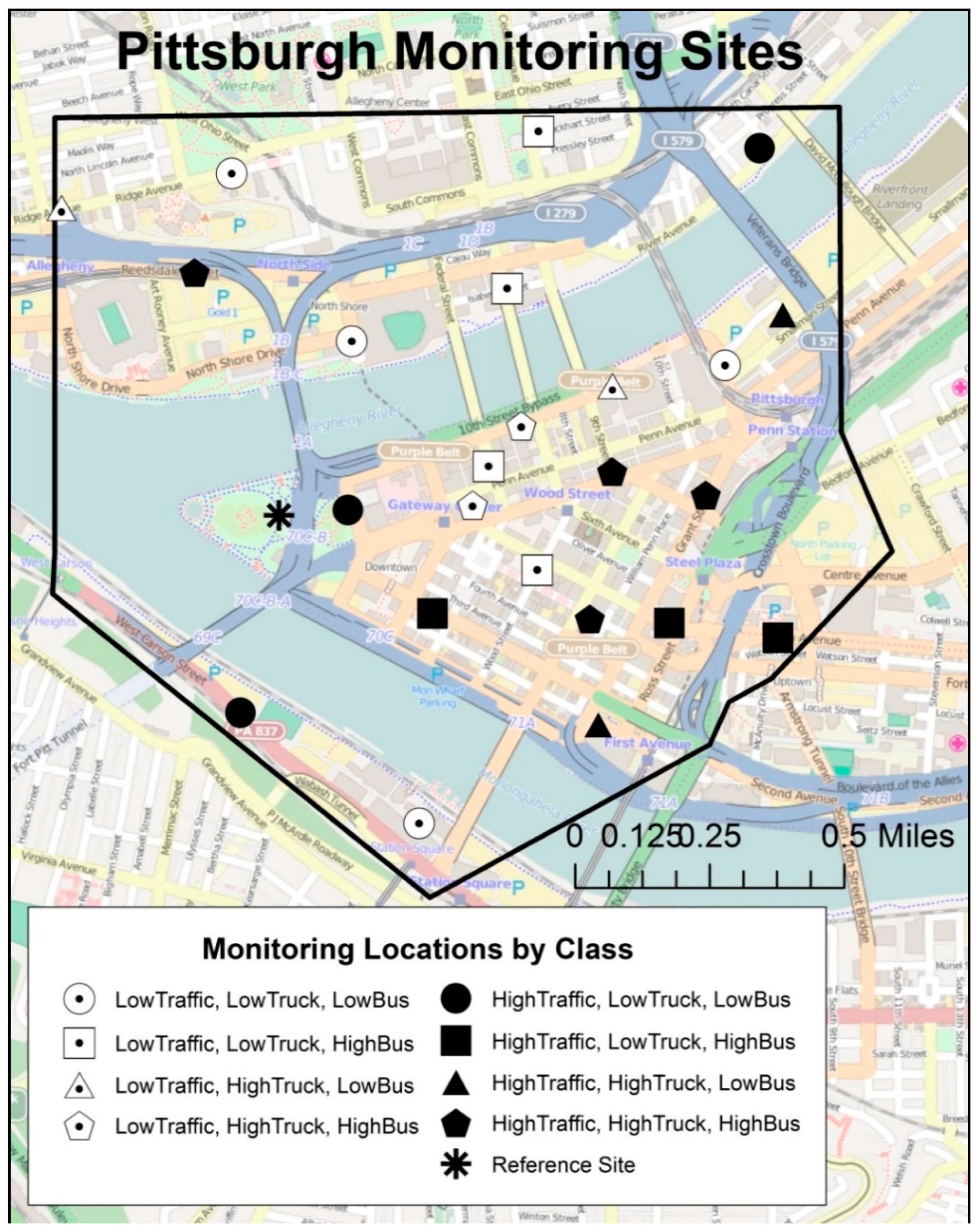
We systematically allocated twenty-four (24) air monitoring sites, using previously-developed geographic information system (GIS)-based methods, to characterize variation in total traffic, buses, and truck traffic across our small domain [
1]. The same sites were sampled in both summer and winter, and were randomly distributed over four 5-day (Monday through Friday) sampling sessions. At each site, we collected paired work-week and rush-hour samples for a suite of gasoline- and diesel-related pollutants. Temporally-adjusted concentrations at each site, for each season, were derived using time trends observed at two reference monitors (one urban and one rural background site). This study design is further detailed, and maps of the reference sites provided, in Tunno et al., [
1].
2.1. Study Domain
We used GIS to fit a polygon that included downtown Pittsburgh, with a uniform elevation of roughly 300 m, to encompass vehicular traffic across highways and bridges surrounding the downtown core, resulting in a sampling domain of roughly 2.8 km
2 (
Figure 1).
2.2. Tracer Selection
We identified chemical tracers for key pollution sources of interest (i.e., heavy trucks, buses, and gasoline vehicles). We collected integrated samples of PM
2.5, BC, trace elements, and organic compounds (PAHs, hopanes, steranes). We also identified elemental constituents found to be associated with diesel emissions in at least two published studies (Al [
16,
17], Ca [
18,
19,
20], and Fe [
20,
21]), based on our previous literature search, and included additional elements related to vehicular emissions, brake/tire wear, soil/road dust resuspension, steel-making, and coal [
22]. We selected organic markers previously identified in diesel exhaust, quantifiable using thermal desorption gas-chromatography mass-spectrometry (TD-GC-MS) [
15], and relatively lower volatility and reactivity relative to other components of diesel exhaust [
9]. Additional information on organic compound marker selection and quartz filter handling is detailed in Tunno et al. [
1].
2.3. Sampling Intervals
Paired samplers ran two (2) programs: one to capture full work-week concentrations (Monday through Friday, 7 a.m. to 7 p.m.), and one to capture rush-hours (Monday through Friday, 5 a.m. to 10 a.m. and 3 p.m. to 7 p.m.). These “rush-hours” were identified as the hours with the heaviest bus and truck traffic, based on the Pennsylvania Department of Transportation (PennDOT) hourly traffic counts and Allegheny County Port Authority bus schedules for the downtown area. Winter sampling was performed from 13 January to 7 February, and summer sampling from 7 July to 1 August 2014.
2.4. Instrumentation
We used programmable, portable ambient air sampling units [
23] which included Harvard Impactors (HI) (Air Diagnostics and Engineering, Inc., Harrison, ME, USA) with 37 mm Teflon filters (PTFE membrane, 2 µm pores, Pall Life Sciences (Port Washington, NY, USA), and HOBO data loggers for temperature and relative humidity (Onset Computer Corporation, Bourne, MA, USA). Battery-operated vacuum pumps (SKC, Inc., Eighty-Four, PA, USA) maintained a flow rate of 4 L per minute (LPM). Particle sampling instruments were housed in weather-tight Pelican boxes.
We adapted these sampling units to collect integrated samples of organic compounds. In separate weather-tight Pelican boxes, additional PM
2.5 samples to analyze for organic compounds were collected using cyclones (Air Diagnostics and Engineering, Inc., (Harrison, ME, USA)) using 37 mm quartz fiber filters (Pallflex Tissuquartz non-heat treated filters, Pall Life Sciences), pre-baked at 900 deg F prior to sampling to remove VOC contamination which may interfere with collection of organic particle components. All samplers were mounted approximately 3 m above ground, near the human breathing zone, but sufficiently out-of-reach to avoid tampering. Most importantly, the sampling height was consistent across all sites, for comparability. Organics samplers were strictly deployed on metal poles, to avoid contamination by VOCs from treated wooden poles [
24].
To enable comparisons of elemental vs. organic, and rush-hour vs. work-week, samples, four (4) monitors were deployed together. Two sampling units collected PM2.5, BC, and trace elements on Teflon filters using Harvard Impactors (HIs); two additional units collected organic compounds using cyclones. One unit of each type was programmed to capture work-week hours, and the other to capture only rush hours. Because four sampling units could not be placed on the same utility pole without obstructing each other, we selected, as needed, the closest suitable pole for the HI (Teflon) samplers, and used the original pole for the cyclone (quartz) samplers.
2.5. Site Selection and Allocation
We aimed to capture the spatial variability in traffic, particularly with regard to diesel- and gasoline-powered vehicles, by allocating sites using three GIS-based indicators: total traffic density, total truck density, and bus route frequency, as described in Tunno et al. [
1]. To compare rush-hour and work-week paired samples, we modified the original site allocation to enable paired sampling. For phase 2, we retained 24 distributed sites from the original 36 sites (66%) for spatial and source variation (
Figure 1). Sites were eliminated (
n = 12 sites) based on similarity in temporally-adjusted organic concentrations with those detected at nearby sampling locations during the Phase 1 summer and winter campaigns [
1], to maximize the retained spatial variation in concentrations across the study area. We retained two reference sites (one upwind background site, one urban site within the domain).
2.6. Laboratory Analyses:
Using an ultramicrobalance (Mettler Toledo Model XP2U, Columbus, OH, USA), Teflon filters were pre- and post-weighed in a temperature and relative-humidity controlled glove box (PlasLabs Model 890 THC, Lansing, MI, USA) to determine total PM
2.5 mass. Reflectometry for BC absorbance was performed using an EEL43M Smokestain Reflectometer (Diffusion Systems, Ltd., London, UK). Inductively-coupled plasma mass spectrometry (ICP-MS) analyses were conducted for elemental constituents by the Wisconsin State Laboratory of Hygiene following documented protocols (ESS INO Method 400.4; EPA Method 1638) [
25]. For OC and EC, thermal-optical reflectance was run by Desert Research Institute (DRI, Reno, NV, USA) [
26], and TD-GC-MS was conducted for organic compounds [
27,
28].
2.7. Quality Assurance and Quality Control
Multiple laboratory and field blanks were collected each session to quantify contamination, on both filter types. Pump flow rates were calibrated to 4.0 LPM, temperature-adjusted based on average forecasted temperatures for the sampling period, and re-assessed after sampling completion. All sampling pumps met acceptable pre- and post-collection flow rates, within ± 5% of 4.0 LPM. A small number of sites (n = 2 for Teflon filters, n = 2 for quartz filters) were re-sampled due to equipment failure during the scheduled session. Field blanks from the same session were used to blank-correct all pollutant concentrations. Data completeness was 96 to 100% for interval- and season-specific sampling campaigns, with no statistical outliers (outside of ±3 standard deviations). One summer work-week PM2.5 sample was lost due to field equipment error. One additional trace element sample was lost due to analytic equipment error.
2.8. GIS-Based Source Density Indicators
We examined both rush-hour and work-week data using the GIS-based source covariates and modifiers reported in Tunno et al. [
1]. All covariates were created using ArcInfo Version 10.2 (ESRI, Redlands, CA, USA). Buffer-based covariates were created for concentric radial buffers surrounding each monitoring location (25 to 200 m), to assess impacts of sources at various distances on observed pollutant concentrations. Buffers larger than 200 m were not considered, because these buffers overlapped between neighboring sites, dampening variance across sites.
2.9. Temporal Adjustment
Using both the rural and urban reference sites, we temporally-adjusted all samples to account for between-session variability driven by time-varying meteorology or long-range pollutant transport. We estimated the expected seasonal average concentration at each site by dividing the observed concentration by the session-specific average concentration from both reference sites, then multiplied the result by the seasonal average concentration from both reference sites, as detailed in Shmool et al. [
29].
2.10. Statistical Analysis
We calculated descriptive statistics for PM
2.5, BC, total EC and OC, trace elements previously associated with diesel emissions (Al, Ca, Fe), and organic compounds, and compared temporally-adjusted pollutant concentration distributions across the source indicator strata used for site selection. We compared pollutant concentrations within sites, by season and by sampling interval (i.e., rush-hour vs work-week), using paired
t-tests. We identified potential statistical outliers (outside of mean ± 3 standard deviations) within each sampling session. Before LUR modeling, bivariate source-pollutant correlations were performed to select candidate source terms, and each source indicator (
Table 1) was assessed individually as a predictor of each temporally-adjusted pollutant concentration. Data analysis and model-building were performed separately for each pollutant by rush and work-week programs, and for summer and winter seasons.
LUR models were derived, for each of the pollutants described above, using manual forward step-wise linear regression, predicting raw pollutant concentrations for the summer and winter seasons, using an adapted version of the modeling approach in Tunno et al. [
9]. In model building, temporal trends in pollutant concentrations were incorporated first into LUR models, using the session-specific mean reference concentration. Source terms with the strongest univariate correlation to the temporally-adjusted pollutant were then incorporated, individually in descending order by strength of the bivariate correlation. Regression models were sequentially fit to assess overall model improvement at each stage, using the coefficient of determination (R
2), and removing non-significant covariates in order of descending
p-value, until all independent terms were significant (
p < 0.05). Covariates were removed, at any stage, if the variance inflation factor (VIF) became greater than 2.0, to reduce multicollinearity between variables.
LUR model residuals were mapped to identify systematic spatial variation and locations poorly predicted by LUR, suggesting the need to identify and incorporate additional covariates. Semivariograms of residuals were created in GIS, and spatial autocorrelation in residuals was tested using the Moran’s I statistic.
2.11. Sensitivity Analyses
Covariate selection was sensitivity-tested using scatterplots to assess fit between each significant predictor and raw pollutant concentrations, to ensure that selected candidate covariates captured variability across the range of concentrations, and that associations were not reliant on outliers or influential points. Tree structures and Random Forest automated methods were performed to corroborate covariate selection. A scatterplot of each retained term was tested against the residual of the prior model in the sequential model-building process to check for outliers and overall fit. We examined model residuals to ensure normality. Backwards elimination, from multivariate linear models including all source covariates with significant bivariate associations with temporally-adjusted concentrations, was used to further corroborate model structure and covariate selection. For validation of LUR predictions, a random 20% of sites (n = 5) were removed from the analysis, and the LUR model was re-fit and used to predict pollutant concentrations at withheld sites. Analyses were performed in SAS v 9.4 (SAS Institute Inc., Cary, NC, USA), ArcInfo, v 10.1 (ESRI, Redlands, CA, USA), R statistical software v 3.1.2, and Excel 2010 (Microsoft, Inc. Redmond, WA, USA).
3. Results
3.1. Summary Statistics and Spatial Patterns
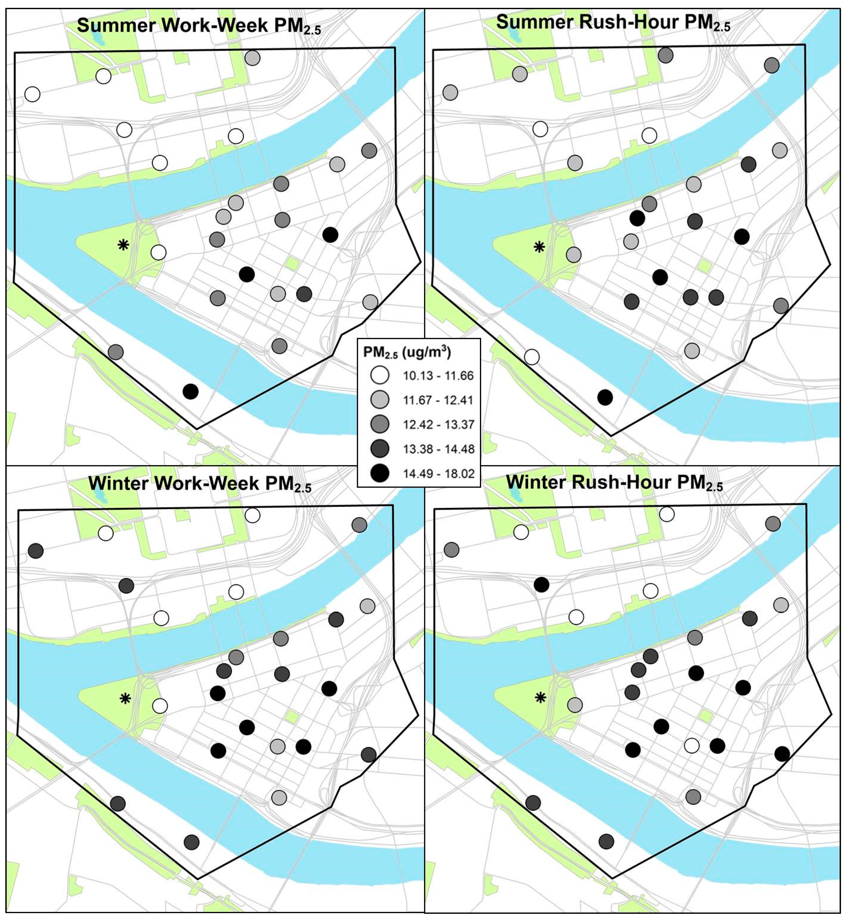
We found no significant differences in total PM
2.5 concentrations, either by season or sampling scheme. Spatial patterning in PM
2.5 for each season was similar, with generally higher concentrations in the center of downtown. Notably, differences in concentrations of PM
2.5 were greater across sites than between seasons. In both seasons, we found higher average PM
2.5 concentrations during rush-hours than over the full work-week (
Table 1). There were no apparent spatial differences in PM
2.5 or constituent concentrations by sampling scheme or season (
Figure 2 and
Figure 3, other constituent maps not shown).
3.2. Comparisons between Sampling Schemes
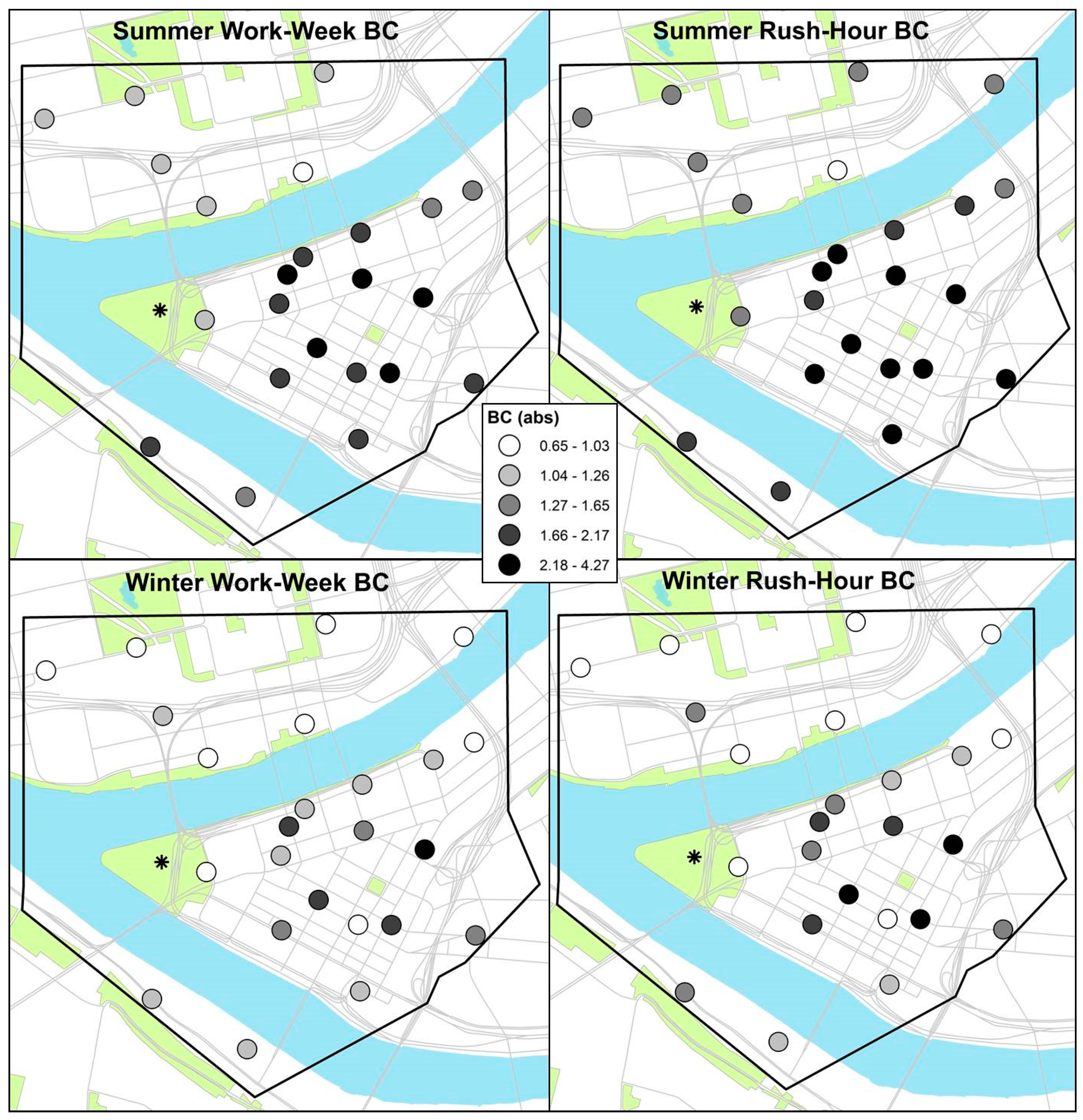
During winter, we found greater concentrations of
diesel-related (i.e., BC, EC, benz(a)anthracene, benzo(e)pyrene, and chrysene) and
traffic/road dust-related constituents (e.g., copper, manganese, potassium, zinc) in rush-hour vs. full work-week samples (
Table 1). Conversely, hopane (
diesel) and arsenic (
coal) concentrations were higher in work-week than rush-hour samples.
During summer, we found greater concentrations of some diesel-related constituents (i.e., BC, fluoranthene, pyrene, cholestane) in rush-hour vs. work-week samples, though some (i.e., hopanes) were higher in work-week samples (
Table 2).
3.3. Comparisons between Seasons
In rush-hour samples, concentrations of
coal-related elements (i.e., As, Se) were higher during summer.
Motor-vehicle-related elements (i.e., calcium, phosphorus, potassium, zinc) and
diesel-related organics (i.e., benzo(e)pyrene, benzo(ghi)perylene, pyrene, total PAHs) were higher during winter (
Supplementary Materials Table S1).
Likewise, in the work-week samples, concentrations of
motor vehicle-related zinc, and
diesel-related organics (i.e., benzo(e)pyrene, benzo(ghi)perylene, chrysene, fluoranthene, pyrene, total PAHs) were higher during winter than summer (
Supplementary Materials Table S2).
3.4. LUR Models
For PM
2.5 and EC, the only significant source covariate retained in LUR models, for both seasons and sampling schemes, was mean bus density within 200 m of the sampling site (
Table 3 and
Table 4). For BC, mean bus density was the strongest term for both seasons and sampling schemes; truck density within 200 m explained additional spatial variability in summer.
For OC, bus stop use (number of stops per day) was the only significant predictor, for both sampling schemes, during winter (
Table 3). During summer, truck density explained variability in rush-hour samples; commercial land use and buildings aspect ratio explained variability in work-week samples (
Table 4).
For total PAHs, bus-related covariates were significant for both seasons and schemes (
Table 3 and
Table 4). For total hopanes, bus density explained spatial variance in full work-week samples, in both seasons. For rush-hour samples, no source covariates predicted spatial variance during winter; only truck density explained spatial variance in summer.
For the elemental tracers (Al, Ca, Fe), during winter, no covariates explained spatial variance in Al or Fe, using either sampling scheme (
Table 3). For Ca, distance to primary road explained variability in rush-hour samples; bus density explained variation in work-week samples. During summer, for all three elements, truck density explained spatial variation in rush-hour samples (
Table 4). No source covariates explained spatial variation in summer work-week samples of Al or Ca; length of roadway explained spatial variability in work-week Fe.
3.5. Sensitivity Analyses
Scatterplots revealed that final models were not driven by outliers or influential points. Tree structures and Random Forest automated methods corroborated the covariates retained in final models. Moran’s I results indicated no spatial autocorrelation in model residuals across distributed monitoring sites. Removal of a random subset (20%) of monitoring sites did not significantly change any of the models, and predicted concentrations at the withheld sites were within 10% of the measured concentrations.
4. Discussion
Air pollution saturation studies are now commonly used in exposure assessment and environmental epidemiology, but few have been able to capture spatial variation during selected hours of the day (e.g., rush-hours, inversion events [
9]), largely due to technical and equipment limitations. Further, relatively few studies to date have been able to incorporate organic pollutants into spatial saturation studies. We sampled gasoline and diesel-related organic and elemental constituents during rush-hour and work-week hours, to disentangle a complex mix of sources impacting spatial variation in air pollution exposures across an urban core.
This study is the first, to our knowledge, to explicitly capture and compare spatial variation in multiple pollutants during high diesel source-intensity hours (“rush hours”) vs. the overall work-week. We hypothesized heightened concentrations and sharper spatial contrasts in multiple pollutants during the rush hours, and expected to identify source terms which differently explained spatial variation in multiple pollutant concentrations during these different hours of the day. Rush-hour sampling indicated non-significantly higher PM2.5 concentrations compared to work-week sampling, in both seasons, with no evident difference in spatial patterns—possibly suggested that rush-hours emissions accounted for a large portion of total PM2.5 concentrations and spatial variance across the downtown core.
We observed higher concentrations of traffic-related elemental and organic constituents during rush-hours, relative to the work-week, again with similar spatial patterning using both sampling schemes. The differences between rush hours and the full work week were stronger for BC and other components than for PM
2.5—possibly because BC and other components may be more specific to traffic and diesel emissions than is total PM
2.5 [
30,
31].
GIS-based source terms explained similar variability (R2) during the rush hours and full work-week, possibly suggesting that the bulk of spatial contrast in diesel-related pollutants may be explained during rush hours. Bus traffic explained the bulk of spatial variance in rush-hour concentrations, and accounted for some spatial variation in work-week samples. Higher concentrations of coal-related elements during work-week, relative to the rush hours, suggests that non-traffic industrial sources may have a greater relative influence on pollution exposure patterns during non-rush-hours.
Comparing between seasons, PM2.5 concentrations did not differ significantly, possibly pointing to the consistency of commuting traffic, working hours, and bus and truck traffic year-round. For BC, EC, and OC, we found higher concentrations during summer compared to winter. The differences between rush hours and the full work week were stronger for BC than for PM2.5—possibly because BC may be more specific to traffic and diesel emissions than is total PM2.5.
Though we hypothesized greater spatial contrasts and different source contributions during rush hours, LUR models for both schemes were comparable for PM2.5 and BC, with bus density as the lone significant predictor. The significance of the bus indicators in predicting concentrations of many pollutants may indicate a greater accuracy in this GIS variable, compared to other source terms, or a particularly strong impact of bus-related emissions. This same pattern held true for total EC rush-hour models in both seasons, as well as winter total OC models, suggesting slightly higher pollutant concentrations and spatial contrasts during rush hours.
We may have observed lesser spatial contrast, and weaker fits for GIS-based source terms, during winter than summer due to a lower mixing height, cooler ambient temperature, and/or greater frequency of inversion events (possibly flattening out spatial contrasts in pollution across this small area of relatively uniform elevation).
There are several limitations to our study, including the lack of downtown-area meteorological data (i.e., windspeed and direction), limiting our ability to account for complex dispersal patterns in and around urban street canyons. In addition, the majority of GIS-based source terms available were based on annual-average source intensity (e.g., annual-average daily traffic)—limiting our ability to identify short-term changes in local emissions during our sampling period. Finally, limited equipment availability required us to sample different sites over several weeks, and to temporally-adjust all concentrations prior to LUR modelling and comparison of spatial patterns. As higher diesel-related exposures are generally found in densely-populated urban areas, diesel particulate matter (DPM) can have a tremendous impact on public health. By performing a saturation sampling campaign across the downtown area during specific time periods (i.e., rush hours), we were able to identify locations and times of peak pollution exposures, and were able to identify potential contributing sources using land use regression modelling. New policies could also be implemented to target specific sources found in the LUR models (e.g., bus routes), to decrease pollutant exposures.
Future studies should consider sampling, as possible, during high- and low-source intensity hours, and include tracers for a wider variety of sources; our study could not, for example, examine impacts of railroads, barges, and other sources, although they may impact upon total diesel-related exposures, and contribute differently to the concentrations of these various constituents. Furthermore, the Pittsburgh Port Authority is changing the majority of their bus fleet to natural gas in the coming years; validation analyses for the effectiveness of this intervention in reducing local concentrations could include re-sampling using this or a similar spatial saturation design.
5. Conclusions
This study is among the most densely-saturated monitoring campaigns, to our knowledge, and was specifically designed to capture spatial variation in pollution during selected hours of the day, incorporating both elemental and organic tracers of diesel-related emissions into our analysis. This method could be replicated across other urban areas to assess whether spatial variation differs by time of day. Future studies could focus on variability in constituents, with an emphasis on local meteorological phenomenon and its impact on spatial gradients in exposure.
Mean bus density was the strongest LUR predictor, regardless of sampling interval, underscoring the significant contribution of bus exhaust to overall pollutant concentrations. While rush-hour sampling produced slightly higher PM2.5 concentrations, there were no evident differences in spatial patterns, compared to work-week sampling, and rush-hour and work-week LUR models explained similar proportions of variability in concentrations in each season. We found substantial spatial variability in most trace elements and organic compounds, with comparable spatial patterns, using both sampling paradigms. Overall, we found higher concentrations of traffic-related trace elements and organic compounds in the rush-hour samples, and higher concentrations of coal-related elements (e.g., As, Se) in the work-week samples. Together, these results indicate that vehicular source patterning during rush hours may account for a substantial portion of overall spatial variation in exposures.
Supplementary Materials
The following are available online at
https://0-www-mdpi-com.brum.beds.ac.uk/1660-4601/15/9/1968/s1, Table S1: Summary and comparison of rush-hour temporally-adjusted pollutant concentrations by winter and summer seasons, Table S2: Summary and comparison of work-week temporally-adjusted pollutant concentrations by winter and summer seasons.
Author Contributions
Data curation, B.J.T., L.C. (Leah Cambal), L.C. (Lauren Chubb) and C.R.; Data analysis, B.J.T., D.R.M., J.L.C.S., S.T. and E.K.; Funding acquisition, J.E.C.; Methodology, B.J.T., Drew Michanowicz, J.L.C.S., S.T. and E.K.; Supervision, J.E.C.; Validation, B.R.T. and J.E.C.; Writing—original draft, B.J.T.; Writing—review & editing, B.J.T., Drew Michanowicz, J.L.C.S., S.T., E.K., L.C. (Leah Cambal), L.C. (Lauren Chubb), C.R. and J.E.C.
Funding
This research was funded by the Allegheny County Health Department (ACHD).
Acknowledgments
This work was supported by the Allegheny County Health Department (ACHD) Clean Air Fund. The authors would like to thank Jayme Graham, Jason Maranche, Darrell Stern, and Jim Thompson for support throughout the project. The authors would like to thank Rebecca Dalton, Sara Gillooly, Jessica McDonald, and R. Tyler Rubright for field work and data support, and Isaac Johnson for GIS support. The authors thank the Pittsburgh Department of Public Works (Alan Asbury and Mike Salem), Duquesne Light Company, and the Allegheny County Department of Parks for monitoring permissions.
Conflicts of Interest
The authors declare no conflict of interest.
References
- Tunno, B.J.; Michanowicz, D.; Tripathy, S.; Chubb, L.; Kinnee, E.; Cambal, L.; Roper, C.; Clougherty, J.E. Spatial Variation in Diesel-Related Elemental and Organic PM2.5 Components during Workweek Hours across a Downtown Core. Sci. Total Environ. 2016, 573, 27–38. [Google Scholar] [CrossRef] [PubMed]
- EPA Diesel Particulate Matter. Available online: http://www3.epa.gov/region1/eco/airtox/diesel.html (accessed on 5 February 2018).
- Sydbom, A.; Blomberg, A.; Parnia, S.; Stenfors, N.; Sandstrom, T.; Dahlen, S.E. Health effects of diesel exhaust emissions. Eur. Respir. J. 2001, 17, 733–746. [Google Scholar] [CrossRef] [PubMed] [Green Version]
- Hesterberg, T.W.; Long, C.M.; Bunn, W.B.; Lapin, C.A.; McClellan, R.O.; Valberg, P.A. Health effects research and regulation of diesel exhaust: An historical overview focused on lung cancer risk. Inhal. Toxicol. 2012, 24, 1–45. [Google Scholar] [CrossRef] [PubMed]
- Kagawa, J. Health effects of diesel exhaust emissions—A mixture of air pollutants of worldwide concern. Toxicology 2002, 181–182, 349–353. [Google Scholar] [CrossRef]
- Ryan, P.H.; LeMasters, G.K. A review of land-use regression models for characterizing intraurban air pollution exposure. Inhal. Toxicol. 2007, 19, 127–133. [Google Scholar] [CrossRef] [PubMed]
- Hoek, G.; Beelen, R.; de Hoogh, K.; Vienneau, D.; Gulliver, J.; Fischer, P.; Briggs, D. A review of land-use regression models to assess spatial variation of outdoor air pollution. Atmos. Environ. 2008, 42, 7561–7578. [Google Scholar] [CrossRef]
- Jerrett, M.; Arain, A.; Kanaroglou, P.; Beckerman, B.; Potoglou, D.; Sahsuvaroglu, T.; Morrison, J.; Giovis, C. A review and evaluation of intraurban air pollution exposure models. J. Expo. Anal. Environ. Epidemiol. 2005, 15, 185–204. [Google Scholar] [CrossRef] [PubMed]
- Tunno, B.J.; Michanowicz, D.R.; Shmool, J.L.; Kinnee, E.; Cambal, L.; Tripathy, S.; Gillooly, S.; Roper, C.; Chubb, L.; Clougherty, J.E. Spatial variation in inversion-focused vs 24-h integrated samples of PM and black carbon across Pittsburgh, PA. J. Expo. Sci. Environ. Epidemiol. 2015. [Google Scholar] [CrossRef]
- Hatzopoulou, M.; Valois, M.F.; Levy, I.; Mihele, C.; Lu, G.; Bagg, S.; Minet, L.; Brook, J. Robustness of Land-Use Regression Models Developed from Mobile Air Pollutant Measurements. Environ. Sci. Technol. 2017, 51, 3938–3947. [Google Scholar] [CrossRef] [PubMed]
- Jedynska, A.; Hoek, G.; Wang, M.; Eeftens, M.; Cyrys, J.; Beelen, R.; Cirach, M.; De Nazelle, A.; Keuken, M.; Visschedijk, A.; et al. Spatial variations of levoglucosan in four European study areas. Sci. Total Environ. 2015, 505, 1072–1081. [Google Scholar] [CrossRef] [PubMed]
- Jedynska, A.G.H.; Wang, M.; Yang, A.; Eeftens, M.; Cyrys, J.; Keuken, M.; Ampe, C.; Beelen, R.; Cesaroni, G.; Forastiere, F. Spatial variations and development of land use regression models of oxidative potential in ten European study areas. Atmos. Environ. 2017, 150, 24–32. [Google Scholar] [CrossRef]
- Gaeta, A.; Cattani, G.; di Bucchianico, A.D.M.; De Santis, A.; Cesaroni, G.; Badaloni, C.; Ancona, C.; Forastiere, F.; Sozzi, R. Development of nitrogen dioxide and volatile organic compounds land use regression models to estimate air pollution exposure near an Italian airport. Atmos. Environ. 2016, 151, 254–262. [Google Scholar] [CrossRef]
- Kheirbek, I.; Johnson, S.; Ross, Z.; Pezeshki, G.; Ito, K.; Eisl, H.; Matte, T. Spatial variability in levels of benzene, formaldehyde, and total benzene, toluene, ethylbenzene and xylenes in New York City: A land-use regression study. Environ. Health 2012, 11, 51. [Google Scholar] [CrossRef] [PubMed]
- Zhu, X.; Fan, Z.-H.; Wu, X.; Meng, Q.; Wang, S.-W.; Tang, X.; Ohman-Strickland, P.; Georgopoulos, P.G.; Zhang, J.; Bonanno, L.; et al. Spatial Variation of Volatile Organic Compounds in a “Hot Spot” for Air Pollution. Atmos. Environ. 2008, 42, 7329–7339. [Google Scholar] [CrossRef] [PubMed]
- Ogulei, D.; Hopke, P.K.; Zhou, L.; Patrick Pancras, J.; Nair, N.; Ondov, J.M. Source apportionment of Baltimore aerosol from combined size distribution and chemical composition data. Atmos. Environ. 2006, 40, 396–410. [Google Scholar] [CrossRef]
- Lough, G.C.; Schauer, J.J. Sensitivity of source apportionment of urban particulate matter to uncertainty in motor vehicle emissions profiles. J. Air Waste Manag. Assoc. 2007, 57, 1200–1213. [Google Scholar] [CrossRef] [PubMed]
- Spencer, M.T.; Shields, L.G.; Sodeman, D.A.; Toner, S.M.; Prather, K.A. Comparison of oil and fuel particle chemical signatures with particle emissions from heavy and light duty vehicles. Atmos. Environ. 2006, 40, 5224–5235. [Google Scholar] [CrossRef]
- Qin, Y.; Kim, E.; Hopke, P.K. The concentrations and sources of PM2.5 in metropolitan New York City. Atmos. Environ. 2006, 40, 312–332. [Google Scholar] [CrossRef]
- Schauer, J.J.; Lough, G.C.; Shafer, M.M.; Christensen, W.F.; Arndt, M.F.; DeMinter, J.T.; Park, J.S. Characterization of metals emitted from motor vehicles. Res. Rep. Health Eff. Inst. 2006, 133, 1–76. [Google Scholar]
- Rizzo, M.J.; Scheff, P.A. Fine particulate source apportionment using data from the USEPA speciation trends network in Chicago, Illinois: Comparison of two source apportionment models. Atmos. Environ. 2007, 41, 6276–6288. [Google Scholar] [CrossRef]
- Tunno, B.J.; Dalton, R.; Michanowicz, D.R.; Shmool, J.L.; Kinnee, E.; Tripathy, S.; Cambal, L.; Clougherty, J.E. Spatial patterning in PM2.5 constituents under an inversion-focused sampling design across an urban area of complex terrain. J. Expo. Sci. Environ. Epidemiol. 2016, 26, 385. [Google Scholar] [CrossRef] [PubMed]
- Matte, T.D.; Ross, Z.; Kheirbek, I.; Eisl, H.; Johnson, S.; Gorczynski, J.E.; Kass, D.; Markowitz, S.; Pezeshki, G.; Clougherty, J.E. Monitoring intraurban spatial patterns of multiple combustion air pollutants in New York City: Design and implementation. J. Expos. Sci. Environ. Epidemiol. 2013, 23, 223–231. [Google Scholar] [CrossRef] [PubMed]
- Gallego, E.; Roca, F.J.; Perales, J.F.; Guardino, X.; Berenguer, M.J. VOCs and PAHs emissions from creosote-treated wood in a field storage area. Sci. Total Environ. 2008, 402, 130–138. [Google Scholar] [CrossRef] [PubMed]
- Sutton, K.L.; Caruso, J.A. Liquid chromatography-inductively coupled plasma mass spectrometry. J. Chromatogr. A 1999, 856, 243–258. [Google Scholar] [CrossRef]
- Chow, J.C.; Watson, J.G.; Pritchett, L.C.; Pierson, W.R.; Frazier, C.A.; Purcell, R.G. The DRI thermal/optical reflectance carbon analysis system: Description, evaluation and applications in U.S. air quality studies. Atmos. Environ. 1993, 27, 1185–1201. [Google Scholar] [CrossRef]
- Chow, J.C.; Yu, J.Z.; Watson, J.G.; Ho, S.S.; Bohannan, T.L.; Hays, M.D.; Fung, K.K. The application of thermal methods for determining chemical composition of carbonaceous aerosols: A review. J. Environ. Sci. Health A 2007, 42, 1521–1541. [Google Scholar] [CrossRef] [PubMed]
- Ho, S.S.; Yu, J.Z.; Chow, J.C.; Zielinska, B.; Watson, J.G.; Sit, E.H.; Schauer, J.J. Evaluation of an in-injection port thermal desorption-gas chromatography/mass spectrometry method for analysis of non-polar organic compounds in ambient aerosol samples. J. Chromatogr. A 2008, 1200, 217–227. [Google Scholar] [CrossRef] [PubMed]
- Shmool, J.L.; Michanowicz, D.R.; Cambal, L.; Tunno, B.; Howell, J.; Gillooly, S.; Roper, C.; Tripathy, S.; Chubb, L.G.; Eisl, H.M.; et al. Saturation sampling for spatial variation in multiple air pollutants across an inversion-prone metropolitan area of complex terrain. Environ. Health 2014, 13, 28. [Google Scholar] [CrossRef] [PubMed] [Green Version]
- Nieuwenhuijsen, M.J.; Donaire-Gonzalez, D.; Rivas, I.; de Castro, M.; Cirach, M.; Hoek, G.; Seto, E.; Jerrett, M.; Sunyer, J. Variability in and Agreement between Modeled and Personal Continuously Measured Black Carbon Levels Using Novel Smartphone and Sensor Technologies. Environ. Sci. Technol. 2015, 26, 385. [Google Scholar] [CrossRef] [PubMed]
- Wang, Y.; Hopke, P.K.; Rattigan, O.V.; Chalupa, D.C.; Utell, M.J. Multiple-year black carbon measurements and source apportionment using delta-C in Rochester, New York. J. Air Waste Manag. Assoc. 2012, 62, 880–887. [Google Scholar] [CrossRef] [PubMed]
© 2018 by the authors. Licensee MDPI, Basel, Switzerland. This article is an open access article distributed under the terms and conditions of the Creative Commons Attribution (CC BY) license (http://creativecommons.org/licenses/by/4.0/).

 ,
, 


