A Nonlinear Inexact Two-Stage Management Model for Agricultural Water Allocation under Uncertainty Based on the Heihe River Water Diversion Plan

Abstract
:1. Introduction
2. Methodology
2.1. Interval Regression Analysis Method
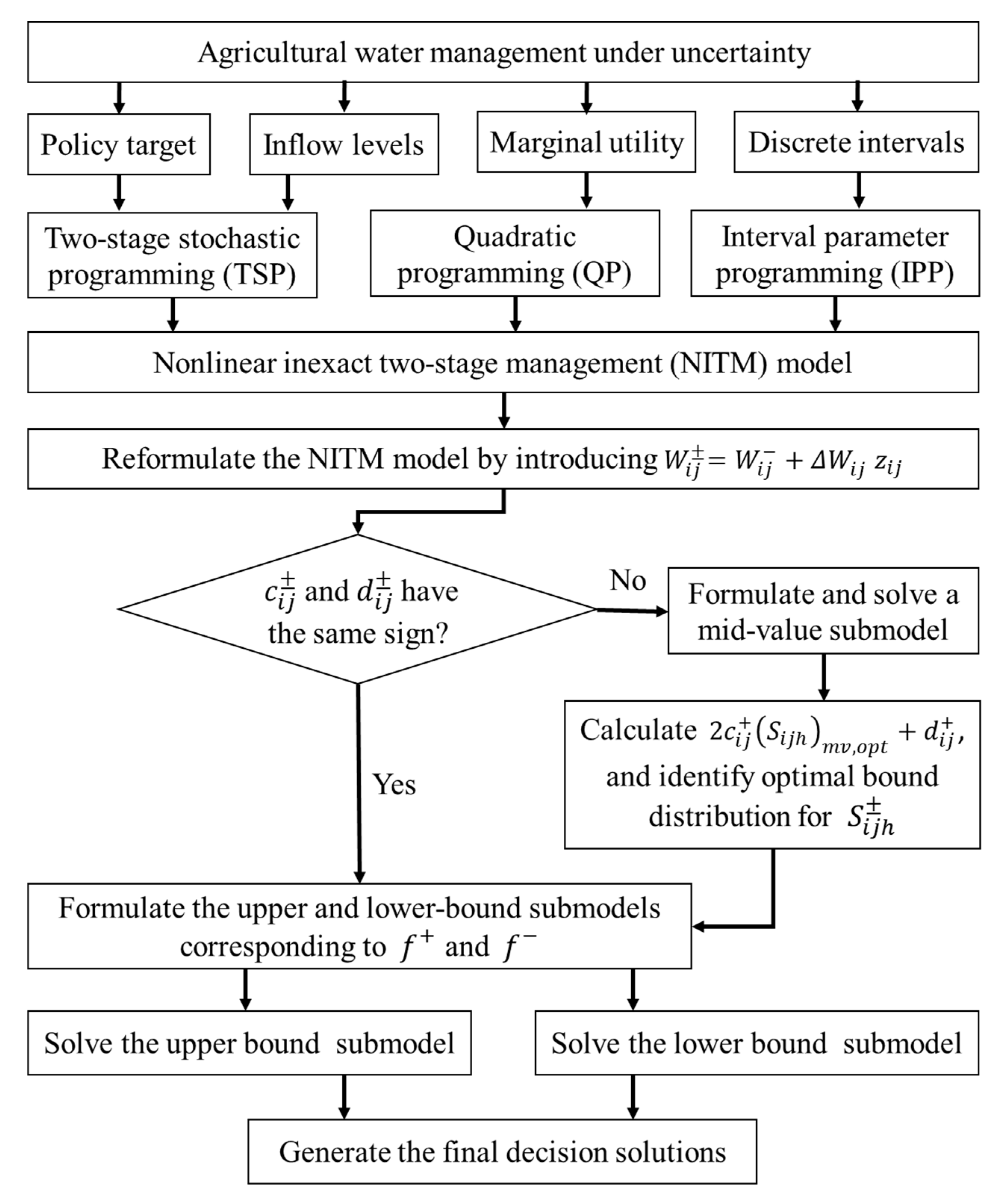
2.2. Nonlinear Inexact Two-Stage Management (NITM) Model
2.3. Solution Method
3. Case Study
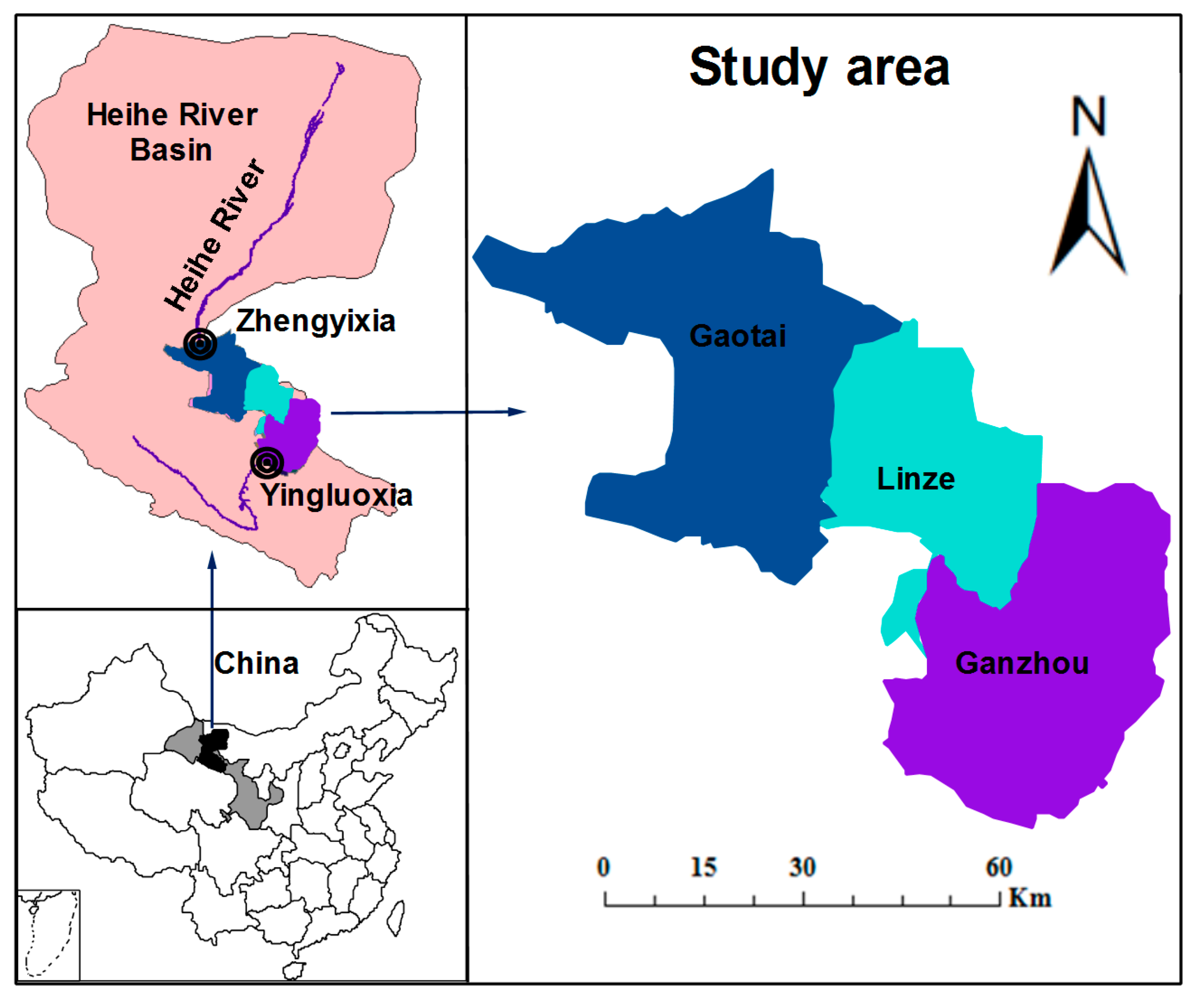
3.1. Study Area
3.2. Data Acquisition and Analysis
3.2.1. Irrigation Targets
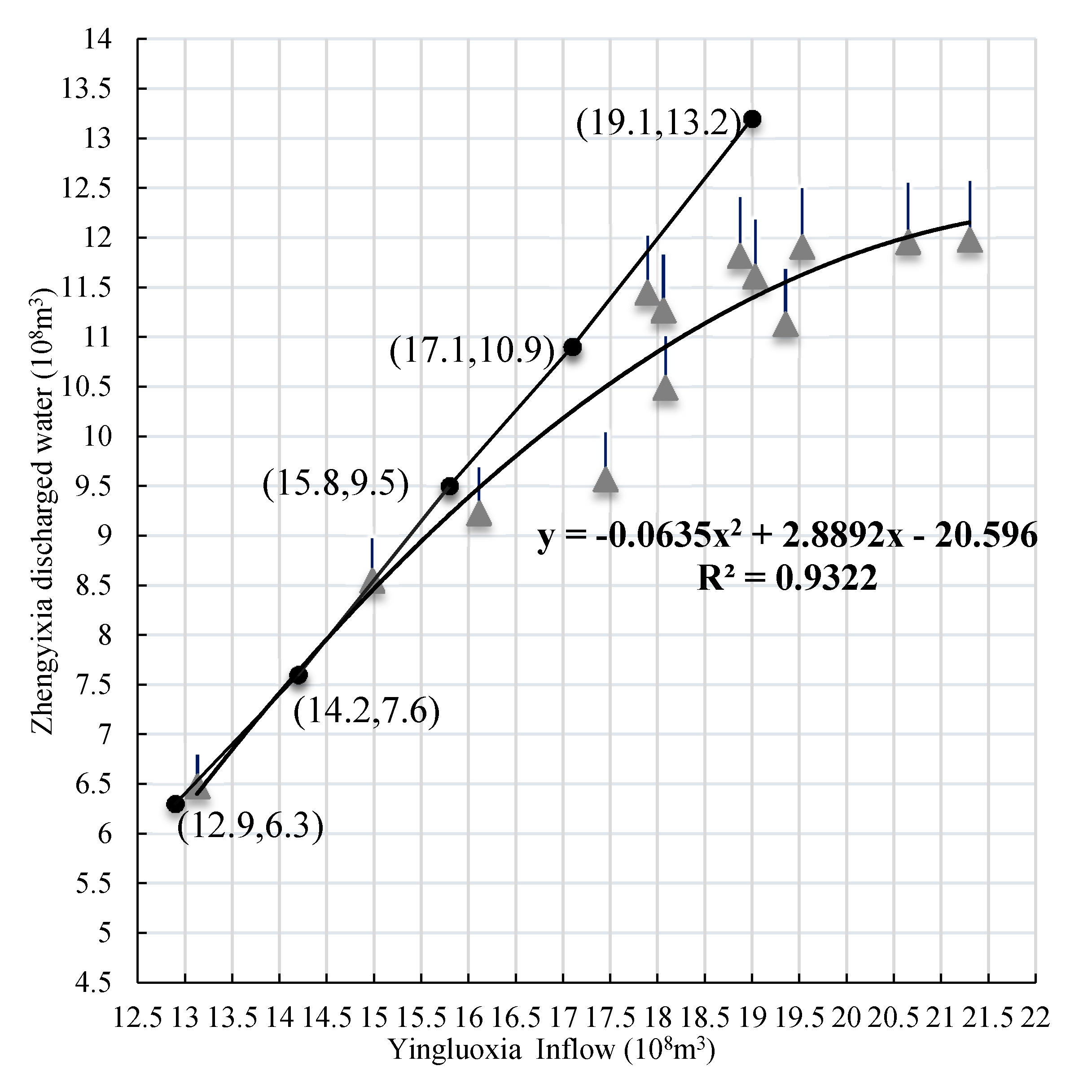
3.2.2. Water Availability
3.2.3. Benefit and Penalty Coefficients
3.3. Nonlinear Inexact Two-Stage Management Model for Optimal Agricultural Water Allocation
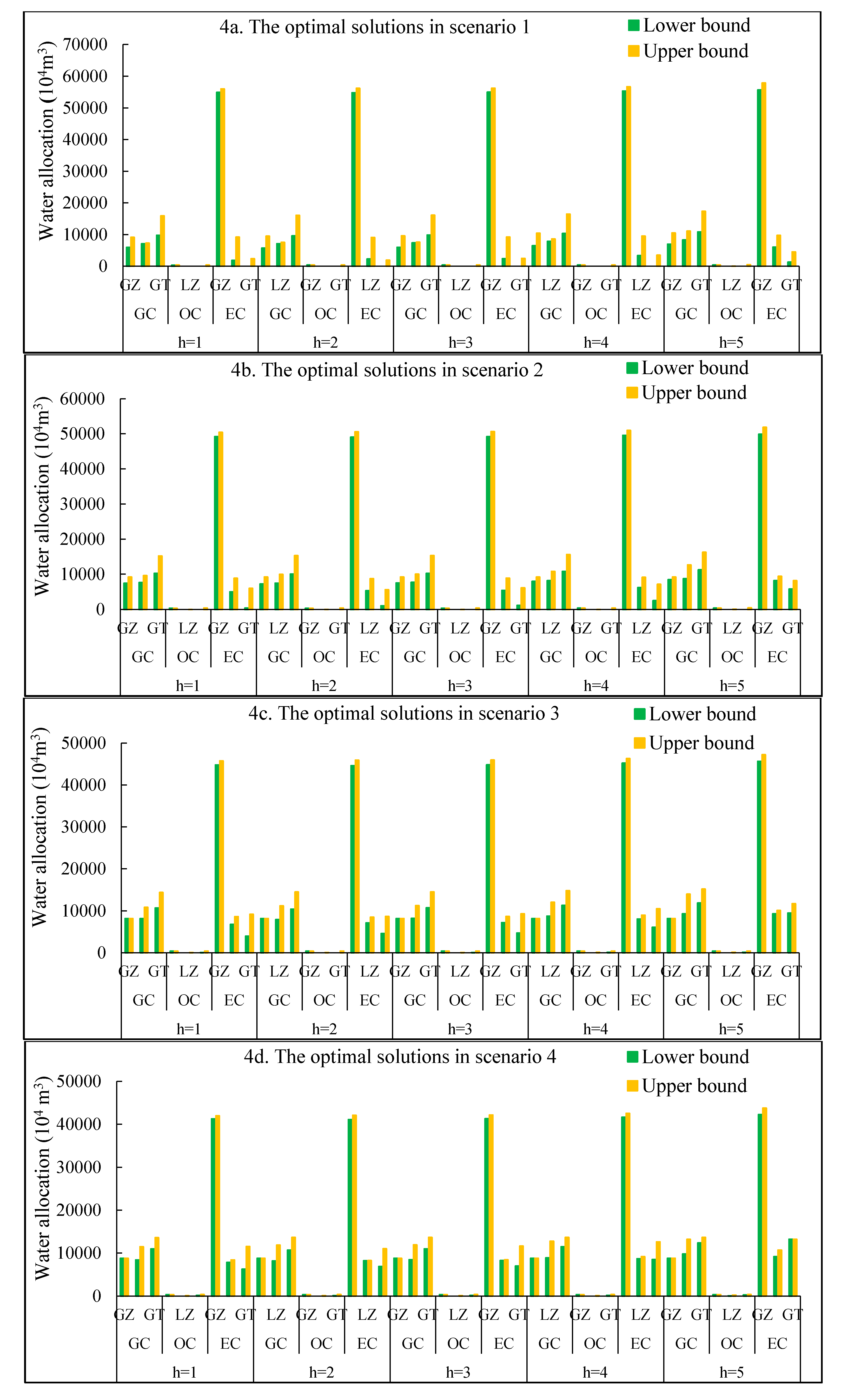
- Scenario 1:
- irrigation targets maintain existing conditions (i.e., ), and the sum of all irrigation targets is the total water consumption in midstream area.
- Scenario 2:
- irrigation targets are reduced by 10%, representing 90% of the current level (i.e., ).
- Scenario 3:
- irrigation targets are reduced by 20%, representing 80% of the current level (i.e., ). This scenario denotes that the total water consumption is reduced by 20%.
- Scenario 4:
- irrigation targets are reduced by 30%, representing 70% of the current level (i.e., ). This scenario represents the case that the total water consumption is reduced by 30%.
4. Results Analysis and Discussion
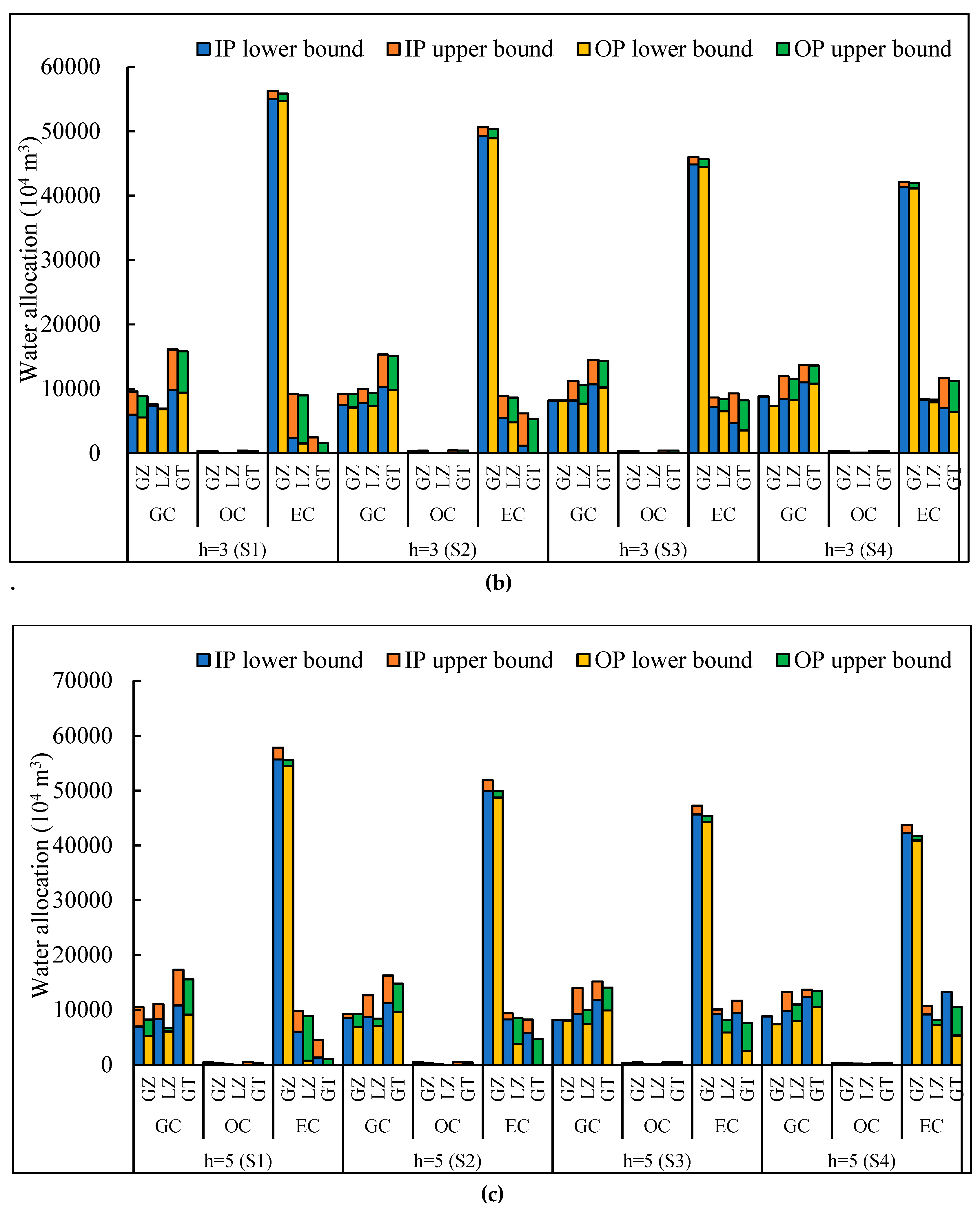
4.1. Optimal Irrigation Water Allocation
4.2. Economic Benefits Analysis
4.3. Discussion
5. Conclusions
Author Contributions
Funding
Acknowledgments
Conflicts of Interest
References
- Chen, Y.; Zhang, D.; Sun, Y.; Liu, X.; Wang, N.; Savenije, H.H.G. Water demand management: A case study of the Heihe River Basin in China. Phys. Chem. Earth Parts A B C 2005, 30, 408–419. [Google Scholar] [CrossRef]
- Zhang, C.; Engel, B.A.; Guo, P.; Zhang, F.; Guo, S.; Liu, X.; Wang, Y. An inexact robust two-stage mixed-integer linear programming approach for crop area planning under uncertainty. J. Clean. Prod. 2018, 204, 489–500. [Google Scholar] [CrossRef]
- Zhao, W.; Liu, B.; Zhang, Z. Water requirements of maize in the middle Heihe River basin, China. Agric. Water Manag. 2010, 97, 215–223. [Google Scholar] [CrossRef]
- Cheng, G.; Li, X.; Zhao, W.; Xu, Z.; Feng, Q.; Xiao, S.; Xiao, H. Integrated study of the water-ecosystem-economy in the Heihe River Basin. Natl. Sci. Rev. 2014, 1, 413–428. [Google Scholar] [CrossRef]
- Li, M.; Guo, P.; Singh, V.P. Biobjective optimization for efficient irrigation under fuzzy uncertainty. J. Irrig. Drain. Eng. 2016, 142, 05016003. [Google Scholar] [CrossRef]
- Zhang, C.; Guo, P. An inexact CVaR two-stage mixed-integer linear programming approach for agricultural water management under uncertainty considering ecological water requirement. Ecol. Indic. 2018, 92, 342–353. [Google Scholar] [CrossRef]
- Smith, D.V. Systems analysis and irrigation planning. J. Irrig. Drain. Div. 1973, 99, 89–107. [Google Scholar]
- Tsakiris, G.; Kiountouzis, E. Optimal intra seasonal irrigation water distribution. Adv. Water Resour. 1984, 7, 89–92. [Google Scholar] [CrossRef]
- Wardlaw, R.; Barnes, J. Optimal allocation of irrigation water supplies in real time. J. Irrig. Drain. Eng. 1999, 125, 345–354. [Google Scholar] [CrossRef]
- Cai, X.; McKinney, D.C.; Rosegrant, M.W. Sustainability analysis for irrigation water management in the Aral Sea region. Agric. Syst. 2003, 76, 1043–1066. [Google Scholar] [CrossRef] [Green Version]
- Cutlac, I.M.; Horbulyk, T.M. Optimal water allocation under short-run water scarcity in the South Saskatchewan River Basin. J. Water Resour. Plan. Manag. 2010, 137, 92–100. [Google Scholar] [CrossRef]
- Singh, A. Simulation-optimization modeling for conjunctive water use management. Agric. Water Manag. 2014, 141, 23–29. [Google Scholar] [CrossRef]
- Inam, A.; Adamowski, J.; Halbe, J.; Prasher, S. Using causal loop diagrams for the initialization of stakeholder engagement in soil salinity management in agricultural watersheds in developing countries: A case study in the Rechna Doab watershed, Pakistan. J. Environ. Manag. 2015, 152, 251–267. [Google Scholar] [CrossRef]
- Smith, P.; House, J.I.; Bustamante, M.; Sobocká, J.; Harper, R.; Pan, G.; West, P.C.; Clark, J.M.; Adhya, T.; Rumpel, C. Global change pressures on soils from land use and management. Glob. Chang. Biol. 2016, 22, 1008–1028. [Google Scholar] [CrossRef] [PubMed]
- Sun, H.; Wang, S.; Hao, X. An improved analytic hierarchy process method for the evaluation of agricultural water management in irrigation districts of north China. Agric. Water Manag. 2017, 179, 324–337. [Google Scholar] [CrossRef]
- Zhao, J.; Li, M.; Guo, P.; Zhang, C.; Tan, Q. Agricultural water productivity oriented water resources allocation based on the coordination of multiple factors. Water 2017, 9, 490. [Google Scholar] [CrossRef]
- Regulwar, D.G.; Gurav, J.B. Irrigation planning under uncertainty—A multi objective fuzzy linear programming approach. Water Resour. Manag. 2011, 25, 1387–1416. [Google Scholar] [CrossRef]
- Huang, G.H. A hybrid inexact-stochastic water management model. Eur. J. Oper. Res. 1998, 107, 137–158. [Google Scholar] [CrossRef]
- Huang, G.H.; Loucks, D.P. An inexact two-stage stochastic programming model for water resources management under uncertainty. Civ. Eng. Syst. 2000, 17, 95–118. [Google Scholar] [CrossRef]
- Maqsood, I.; Huang, G.H.; Yeomans, J.S. An interval-parameter fuzzy two-stage stochastic program for water resources management under uncertainty. Eur. J. Oper. Res. 2005, 167, 208–225. [Google Scholar] [CrossRef]
- Li, Y.P.; Huang, G.H.; Nie, S.L. An interval-parameter multi-stage stochastic programming model for water resources management under uncertainty. Adv. Water Resour. 2006, 29, 776–789. [Google Scholar] [CrossRef]
- Marques, G.F.; Lund, J.R.; Howitt, R.E. Modeling conjunctive use operations and farm decisions with two-stage stochastic quadratic programming. J. Water Resour. Plan. Manag. 2009, 136, 386–394. [Google Scholar] [CrossRef]
- Guo, P.; Huang, G.H.; Zhu, H.; Wang, X.L. A two-stage programming approach for water resources management under randomness and fuzziness. Environ. Model. Softw. 2010, 25, 1573–1581. [Google Scholar] [CrossRef]
- Huang, Y.; Li, Y.; Chen, X.; Ma, Y.G. Optimization of the irrigation water resources for agricultural sustainability in Tarim River Basin, China. Agric. Water Manag. 2012, 107, 74–85. [Google Scholar] [CrossRef]
- Guo, P.; Wang, X.; Zhu, H.; Li, M. Inexact fuzzy chance-constrained nonlinear programming approach for crop water allocation under precipitation variation and sustainable development. J. Water Resour. Plan. Manag. 2013, 140, 05014003. [Google Scholar] [CrossRef]
- Li, M.; Guo, P.; Ren, C. Water resources management models based on two-level linear fractional programming method under uncertainty. J. Water Resour. Plan. Manag. 2015, 141, 05015001. [Google Scholar] [CrossRef]
- Zhang, C.; Guo, P. FLFP: A fuzzy linear fractional programming approach with double-sided fuzziness for optimal irrigation water allocation. Agric. Water Manag. 2018, 199, 105–119. [Google Scholar] [CrossRef]
- Li, M.; Fu, Q.; Singh, V.P.; Liu, D.; Li, X. Stochastic multi-objective modelling for optimization of water-food-energy nexus of irrigated agriculture. Adv. Water Resour. 2019, 127, 209–224. [Google Scholar] [CrossRef]
- Harou, J.J.; Pulido-Velazquez, M.; Rosenberg, D.E.; Medellín-Azuara, J.; Lund, J.R.; Howitt, R.E. Hydro-economic models: Concepts, design, applications, and future prospects. J. Hydrol. 2009, 375, 627–643. [Google Scholar] [CrossRef] [Green Version]
- Jakeman, A.J.; Letcher, R.A. Integrated assessment and modelling: Features, principles and examples for catchment management. Environ. Model. Softw. 2003, 18, 491–501. [Google Scholar] [CrossRef]
- Lund, J.R.; Cai, X.; Characklis, G.W. Economic engineering of environmental and water resource systems. J. Water Resour. Plan. Manag. 2006, 132, 399–402. [Google Scholar] [CrossRef]
- Heinz, I.; Pulido-Velazquez, M.; Lund, J.R.; Andreu, J. Hydro-economic modeling in river basin management: Implications and applications for the European water framework directive. Water Resour. Manag. 2007, 21, 1103–1125. [Google Scholar] [CrossRef]
- Cai, X.M. Implementation of holistic water resources–economic optimization models for river basin management—Reflective experiences. Environ. Model. Softw. 2008, 23, 2–18. [Google Scholar] [CrossRef]
- Brouwer, R.; Hofkes, M. Integrated hydro-economic modelling: Approaches, key issues and future research directions. Ecol. Econ. 2008, 66, 16–22. [Google Scholar] [CrossRef]
- Esteve, P.; Varela-Ortega, C.; Blanco-Gutiérrez, I.; Downing, T.E. A hydro-economic model for the assessment of climate change impacts and adaptation in irrigated agriculture. Ecol. Econ. 2015, 120, 49–58. [Google Scholar] [CrossRef] [Green Version]
- Forni, L.G.; Medellín-Azuara, J.; Tansey, M.; Young, C.; Purkey, D.; Howitt, R. Integrating complex economic and hydrologic planning models: An application for drought under climate change analysis. Water Resour. Econ. 2016, 16, 15–27. [Google Scholar] [CrossRef]
- Mirchi, A.; Watkins, D.W.; Engel, V.; Sukop, M.C.; Czajkowski, J.; Bhat, M.; Rehage, J.; Letson, D.; Takatsuka, Y.; Weisskoff, R. A hydro-economic model of South Florida water resources system. Sci. Total Environ. 2018, 628, 1531–1541. [Google Scholar] [CrossRef] [PubMed]
- Li, Y.P.; Huang, G.H. Inexact multistage stochastic quadratic programming method for planning water resources systems under uncertainty. Environ. Eng. Sci. 2007, 24, 1361–1378. [Google Scholar] [CrossRef]
- Chen, M.; Huang, G.H. A derivative algorithm for inexact quadratic program—Application to environmental decision-making under uncertainty. Eur. J. Oper. Res. 2001, 128, 570–586. [Google Scholar] [CrossRef]
- Gu, B.; Victor, S.S. A solution path algorithm for general parametric quadratic programming problem. IEEE Trans. Neural Netw. Learn. Syst. 2017, 29, 4462–4472. [Google Scholar] [PubMed]
- Tong, F.; Guo, P. Simulation and optimization for crop water allocation based on crop water production functions and climate factor under uncertainty. Appl. Math. Model. 2013, 37, 7708–7716. [Google Scholar] [CrossRef]
- Tanaka, H.; Lee, H. Interval regression analysis by quadratic programming approach. IEEE Trans. Fuzzy Syst. 1998, 6, 473–481. [Google Scholar] [CrossRef]
- Li, D.; Shao, M. Simulating the vertical transition of soil textural layers in north-western China with a Markov chain model. Soil Res. 2013, 51, 182–192. [Google Scholar] [CrossRef]
- Datta, B.; Burges, S.J. Short-term, single, multiple-purpose reservoir operation: Importance of loss functions and forecast errors. Water Resour. Res. 1984, 20, 1167–1176. [Google Scholar] [CrossRef]


| Symbol | Notation |
|---|---|
| f± | System economic benefits (108 Yuan) |
| i | Subarea, i = 1,2,3. I = 3 (i = 1 denotes GZ; i = 2 denotes LZ and i = 3 denotes GT) |
| j | Crop, j = 1,2,3. J = 3 (j = 1 denotes GC; j = 2 denotes OC and j = 3 denotes EC) |
| h | Inflow level, h = 1,2,3,4,5. H = 5 (h = 1, low level; h = 2, low-medium level; h = 3, medium level; h = 4, medium-high level and h = 5, high level) |
| ph | Probability of inflow level h |
| The benefit coefficient, benefit for subarea i to j crop of promised allocated irrigation water (104 Yuan/104 m3) | |
| The slope of the relationship curve between unit benefit and irrigation water amount for subarea i to j crop ( < 0 denotes that unit benefit decrease with irrigation water increase) | |
| The intercept of the relationship curve between unit benefit and the amount of irrigation water for subarea i to j crop (> 0) | |
| The penalty coefficient, reductions/penalties for water users to subarea i for crop j of water not irrigated (104 Yuan/104 m3), | |
| The slope of the relationship curve between unit penalty and the amount of irrigation water shortages for subarea i to j crop ( denotes that as water shortages increase, penalties also increase) | |
| The intercept of the relationship curve between unit penalty and the amount of irrigation water shortages for subarea i to j crop () | |
| Pre-regulated irrigation targets promised to water users for subarea i to j crop. This is the first stage decision variable (104 m3) | |
| Random variable of surface water availability for irrigation under a certain inflow level h (104 m3) | |
| Random variable of groundwater availability for irrigation under a certain inflow level h (104 m3) | |
| ηsw | Irrigation water use efficiency coefficient of surface water, 0.52 |
| ηgw | Irrigation water use efficiency coefficient of groundwater, 0.6 |
| ηag | The proportion of agricultural irrigation in three studied administrative regions to water consumption, 0.9 |
| Water shortages for subarea i to j crop under inflow level h, which is the amount of water that does not satisfy the promised target under the level of total water availabilities (104 m3) | |
| Wijmax | The maximum allowable water for subarea i to j crop (104 m3) |
| zij | Decision variable to solve the NITM model, , and |
| Subarea | Irrigation Targets (108 m3) | ||
|---|---|---|---|
| GC | OC | EC | |
| GZ | [1.05059, 1.2598] | [0.04794, 0.07347] | [5.45679, 6.24537] |
| LZ | [1.88783, 2.14500] | [0.03234, 0.05051] | [1.35234, 1.52921] |
| GT | [1.95183, 2.14411] | [0.05304, 0.06544] | [1.89169, 2.15210] |
| Irrigation quota for each crop (m3/ha) | |||
| GZ | [5595, 7020] | [4320, 5625] | [11232, 12355] |
| LZ | [7500, 9720] | [5175, 6750] | [11659, 12825] |
| GT | [6975, 9840] | [4725, 6150] | [12105, 13316] |
| Maximum allowable water (108 m3) | |||
| GZ | 1.3385 | 0.0767 | 6.3192 |
| LZ | 2.1155 | 0.0527 | 1.6083 |
| GT | 2.3662 | 0.0670 | 2.2892 |
| Inflow Level | Probability | Surface Available Water from the IP | Surface Available Water from the OP | Allowable Groundwater | Total Available Water from the IP | Total Available Water from the OP |
|---|---|---|---|---|---|---|
| Low | 0.12 | 6.79 | 6.60 | [2.20, 2.28] | [8.99, 9.07] | [8.80, 8.88] |
| Low-medium | 0.25 | [6.57, 6.79] | 6.60 | [2.29, 2.44] | [8.86, 9.23] | [8.89, 9.04] |
| Medium | 0.32 | [6.57, 6.60] | 6.30 | [2.45, 2.66] | [9.02, 9.26] | [8.75, 8.96] |
| Medium-high | 0.17 | [6.60, 6.86] | 6.20 | [2.67, 2.77] | [9.27, 9.63] | [8.87, 8.97] |
| High | 0.14 | [6.86, 7.62] | 5.80 | [2.78, 2.88] | [9.64, 10.5] | [8.58, 8.68] |
| Subarea | Upper Bound | Lower Bound | ||||
|---|---|---|---|---|---|---|
| GC | OC | EC | GC | OC | EC | |
| Benefit coefficients when water demand is satisfied () | ||||||
| GZ | −1.0264x + 55955 | −36.1470x + 54614 | −0.2572x + 56610 | −1.0264x + 44890 | −36.1470x + 26294 | −0.2572x + 25803 |
| LZ | −0.8515x + 41516 | −13.7720x + 22893 | −1.1245x + 40698 | −0.8515x + 29228 | −13.7720x + 15844 | −1.3427x + 27671 |
| GT | −0.4149x + 32466 | −26.0970x + 42300 | −0.7311x + 49580 | −0.4149x + 27408 | −27.8260x + 24563 | −0.7311x + 26426 |
| Penalty coefficients when water demand is not satisfied () | ||||||
| GZ | 2.0528x + 95124 | 72.2940x + 92844 | 0.5144x + 96237 | 1.8475x + 68682 | 65.0646x + 40230 | 0.4630x + 39479 |
| LZ | 1.7030x + 70577 | 27.5440x + 38918 | 2.2490x + 69187 | 1.5327x + 44719 | 24.7896x + 24241 | 2.4169x + 42337 |
| GT | 0.8298x + 55192 | 52.1940x + 71910 | 1.4622x + 84286 | 0.7468x + 41934 | 50.0868x + 37581 | 1.3160x + 40432 |
© 2019 by the authors. Licensee MDPI, Basel, Switzerland. This article is an open access article distributed under the terms and conditions of the Creative Commons Attribution (CC BY) license (http://creativecommons.org/licenses/by/4.0/).
Share and Cite
Zhang, C.; Yue, Q.; Guo, P. A Nonlinear Inexact Two-Stage Management Model for Agricultural Water Allocation under Uncertainty Based on the Heihe River Water Diversion Plan. Int. J. Environ. Res. Public Health 2019, 16, 1884. https://0-doi-org.brum.beds.ac.uk/10.3390/ijerph16111884
Zhang C, Yue Q, Guo P. A Nonlinear Inexact Two-Stage Management Model for Agricultural Water Allocation under Uncertainty Based on the Heihe River Water Diversion Plan. International Journal of Environmental Research and Public Health. 2019; 16(11):1884. https://0-doi-org.brum.beds.ac.uk/10.3390/ijerph16111884
Chicago/Turabian StyleZhang, Chenglong, Qiong Yue, and Ping Guo. 2019. "A Nonlinear Inexact Two-Stage Management Model for Agricultural Water Allocation under Uncertainty Based on the Heihe River Water Diversion Plan" International Journal of Environmental Research and Public Health 16, no. 11: 1884. https://0-doi-org.brum.beds.ac.uk/10.3390/ijerph16111884