Spatio-Temporal Prediction for the Monitoring-Blind Area of Industrial Atmosphere Based on the Fusion Network

 ,
,  ,
,
Abstract
:1. Introduction
2. Related Works
2.1. Time Series Prediction Methods
2.2. Spatial Analysis of Atmospheric Environment
3. Fusion Network of Spatio-Temporal Prediction
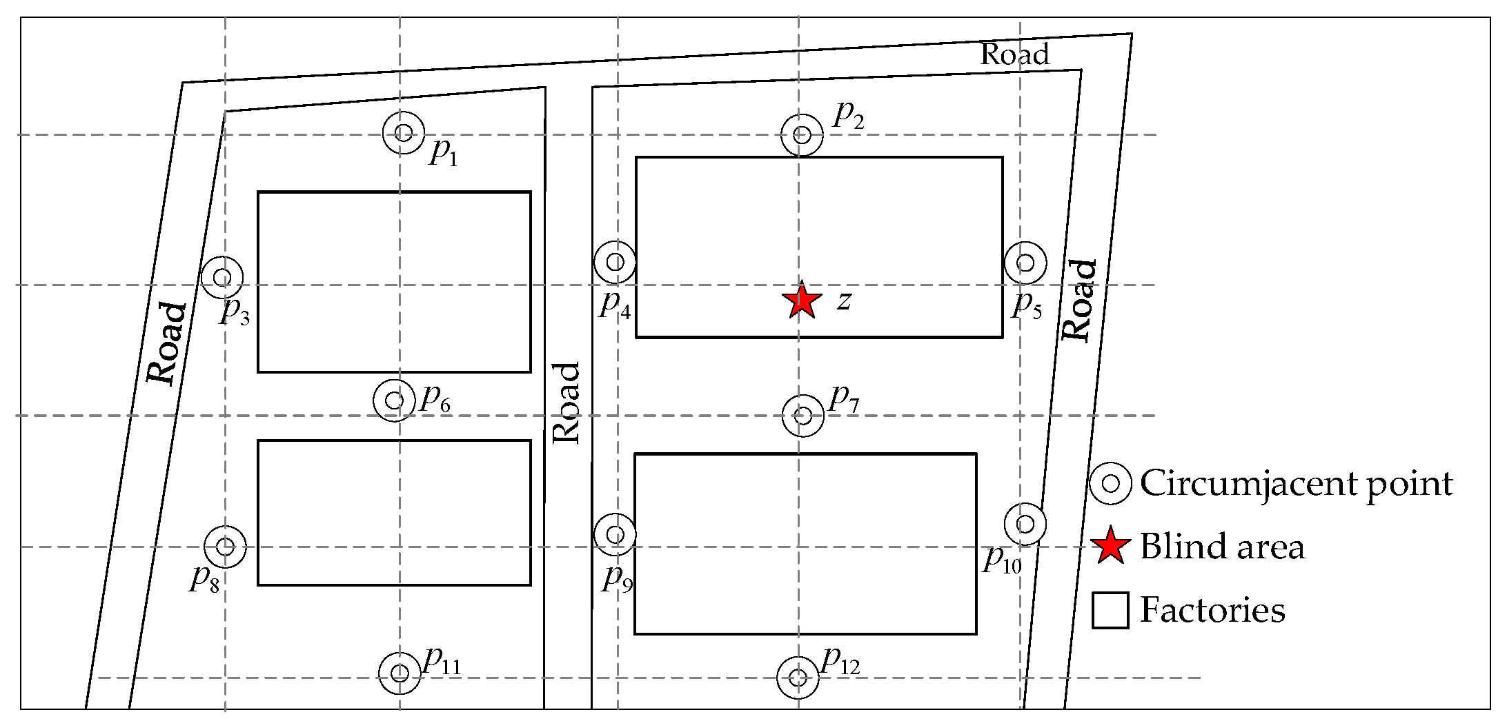
3.1. Problem Description
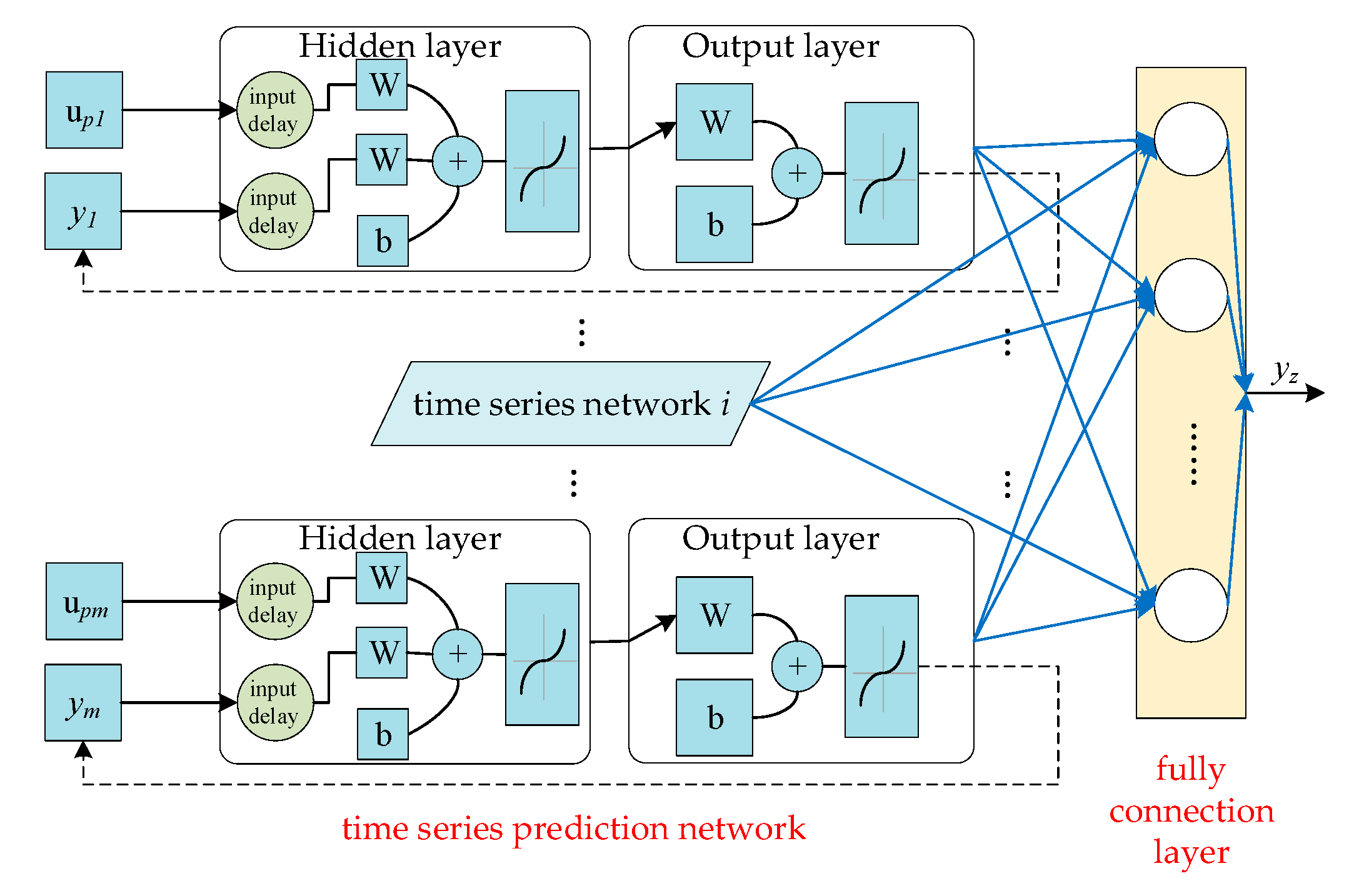
3.2. Fusion Network Framework
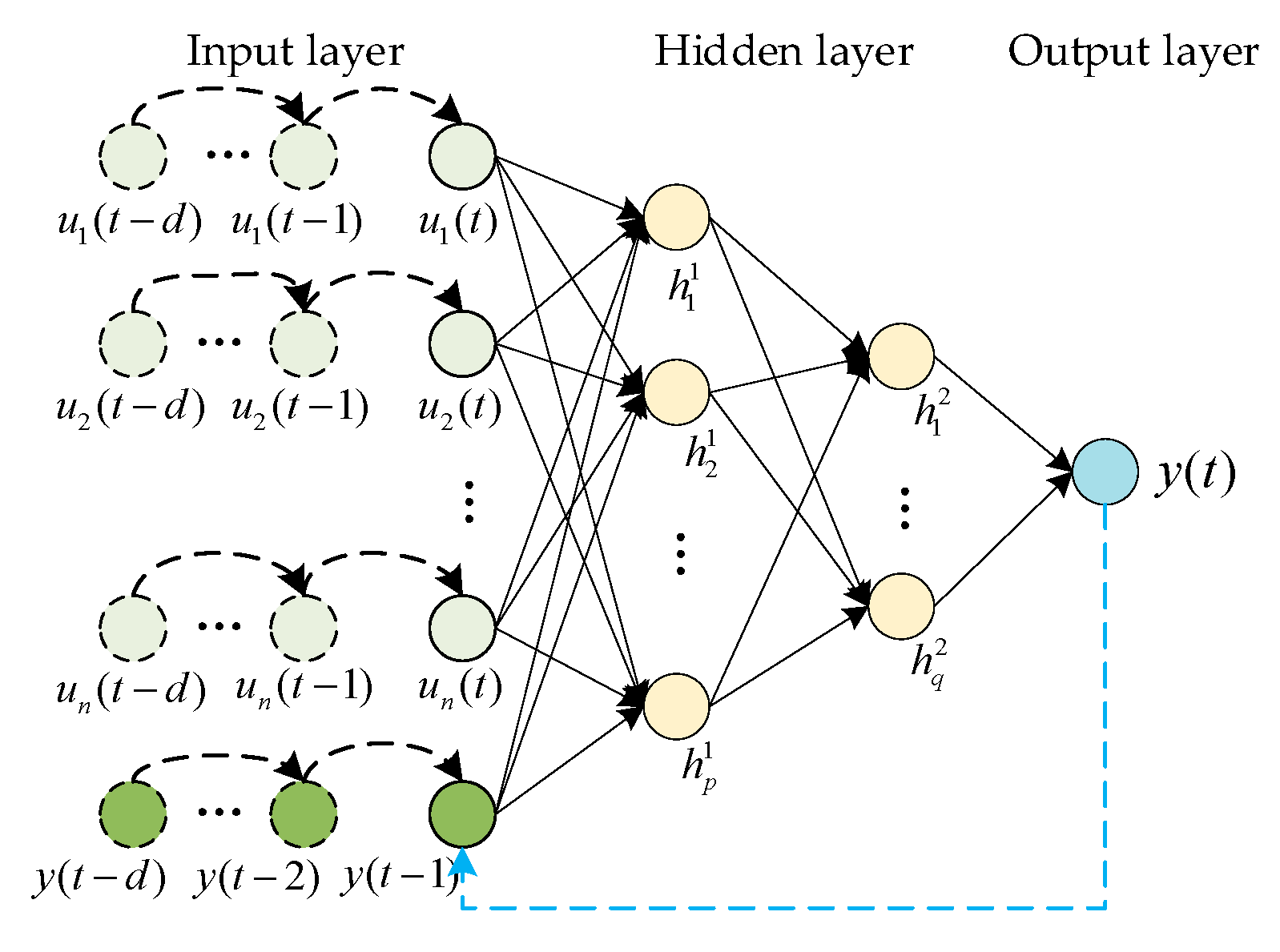
3.3. Time Series Prediction Model Based on NARX
3.4. Spatial Inference Model
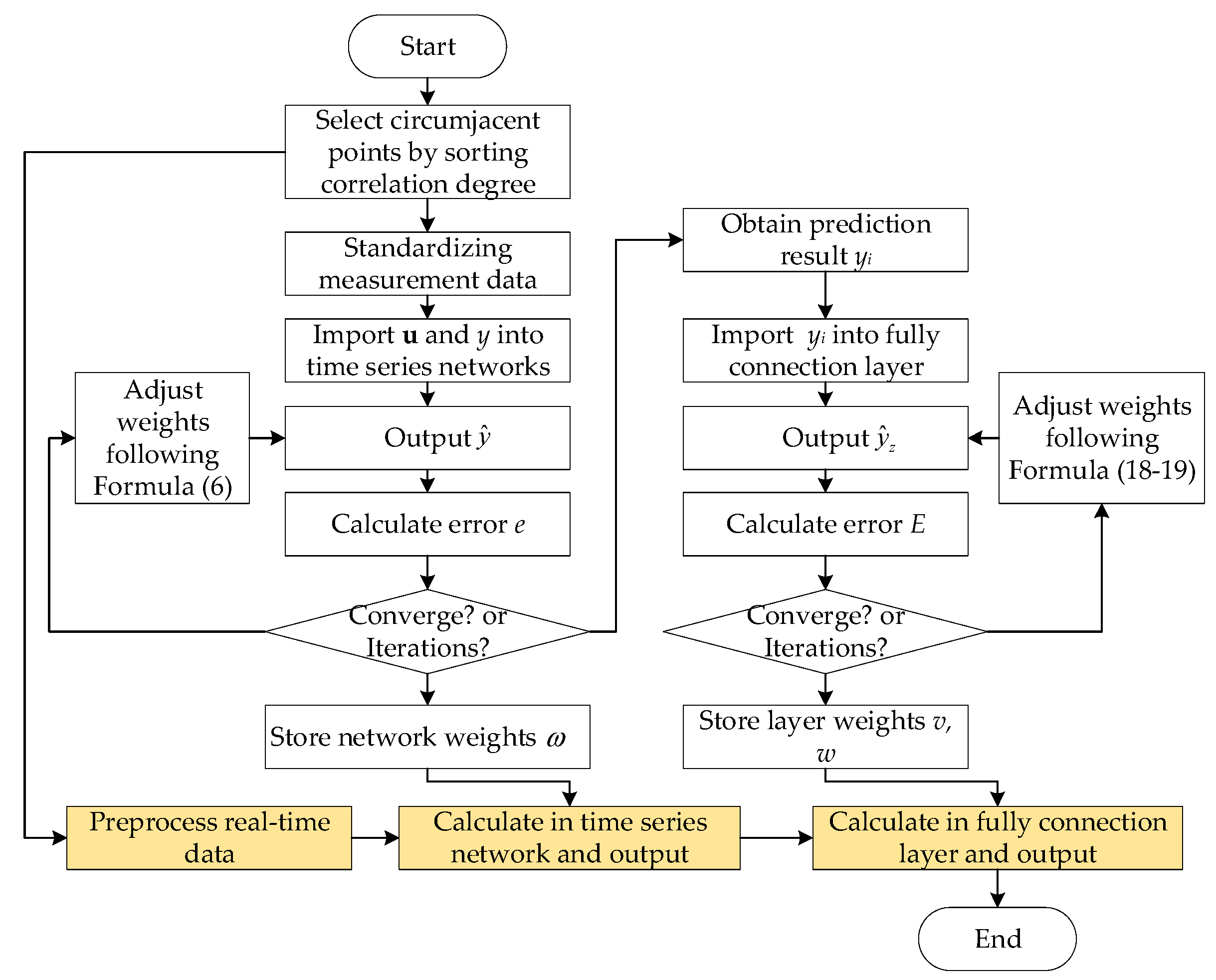
3.5. Spatio-Temporal Prediction Algorithm
4. Experiment and Result
4.1. Experiment Data and Setting
4.2. Experiment Result
5. Discussion
6. Conclusions
Author Contributions
Funding
Conflicts of Interest
References
- Zheng, J. Study on VOCs in atmosphere and their sources of atypical industrial park in Shanghai. J. Shanghai Norm. Univ. (Nat. Sci.) 2017, 46, 298–303. (In Chinese) [Google Scholar]
- Cao, X.; Roy, G.; Hurley, W.J.; Andrews, W.S. Dispersion coefficients for Gaussian puff models. Bound. Layer Meteor. 2011, 139, 487–500. [Google Scholar] [CrossRef]
- Shang, X.; Li, Y.; Pan, Y.; Liu, R.; Lai, Y. Modification and application of gaussian plume model for an industrial transfer park. Adv. Mater. Res. 2013, 785–786, 1384–1387. [Google Scholar] [CrossRef]
- Wang, Y.; Huang, H.; Huang, L.; Ristic, B. Evaluation of Bayesian source estimation methods with Prairie Grass observations and Gaussian plume model: A comparison of likelihood functions and distance measures. Atmos. Environ. 2017, 152, 519–530. [Google Scholar] [CrossRef]
- Overcamp, T.J. An Exact solution for the ground-level gamma dose rate from a spherical Gaussian puff. Health Phys. 2016, 111, 403. [Google Scholar] [CrossRef] [PubMed]
- Gao, J.; King, M.; Lu, Z.; Tjøstheim, D. Specification testing in nonlinear and nonstationary time series autoregression. Ann. Stat. 2009, 37, 3893–3928. [Google Scholar] [CrossRef]
- Liu, Q.; Chung, E.; Zhai, L. Fusing moving average model and stationary wavelet decomposition for automatic incident detection: Case study of Tokyo Expressway. J. Traff. Transp. Eng. 2014, 1, 404–414. [Google Scholar] [CrossRef]
- Chen, J.; Wang, W.; Huang, C. Analysis of an adaptive time-series autoregressive moving-average (ARMA) model for short-term load forecasting. Electr. Power Syst. Res. 1995, 34, 187–196. [Google Scholar] [CrossRef]
- Nelson, B.K. Statistical methodology: V. Time series analysis using autoregressive integrated moving average (ARIMA) models. Acad. Emerg. Med. 2014, 5, 739–744. [Google Scholar] [CrossRef]
- Eknath, K.G.; Muley, A.A.; Deshmukh, N.K.; Bhalchandra, P.U. Autoregressive integrated moving average time series model for forecasting air pollution in Nanded city, Maharashtra, India. Model. Earth Syst. Environ. 2018, 4, 1435–1444. [Google Scholar]
- Wang, Y.; Wang, C.; Shi, C.; Xiao, B. Short-term cloud coverage prediction using the ARIMA time series model. Remote Sens. Lett. 2018, 9, 275–284. [Google Scholar] [CrossRef]
- Yang, H.; Pan, Z.; Bai, W. Review of time series prediction methods. Comput. Sci. 2019, 46, 21–28. (In Chinese) [Google Scholar]
- Botvinick, M.M.; Plaut, D.C. Short-term memory for serial order: A recurrent neural network model. Psychol. Rev. 2006, 113, 201–233. [Google Scholar] [CrossRef] [PubMed]
- Graves, A.; Fernández, S.; Schmidhuber, J. Multi-dimensional recurrent neural networks. In Proceedings of the International Conference on Artificial Neural Networks, Berlin, Germany, 9 September 2007; pp. 549–558. [Google Scholar]
- Schuster, M.; Paliwal, K.K. Bidirectional recurrent neural networks. IEEE Trans. Signal Process. 1997, 45, 2673–2681. [Google Scholar] [CrossRef] [Green Version]
- Hochreiter, S.; Schmidhuber, J. Long short-term memory. Neural Comput. 1997, 9, 1735–1780. [Google Scholar] [CrossRef] [PubMed]
- Xie, Y.; Han, X.; Li, Q. Research on applied-information technology with PM2.5 generation and evolution model based on BP neural network. Adv. Mater. Res. 2014, 1003, 4. [Google Scholar] [CrossRef]
- Wang, M.; Yuan, Z.; Zhang, X.; Zheng, D.; Ji, D. Construction of air quality evaluation system based on FCM algorithm and BP neural network. Agric. Biotechnol. 2018, 7, 279–281. [Google Scholar]
- Zhang, J.; Liu, Y.; Gu, F.; Shen, L.; Mao, X.; Wu, J.; Wang, C.; Bao, Z. The humidity compensation for measurement systems of aerosol mass concentrations based on the PSO-BP neural network. Chin. J. Sens. Actuators 2017, 30, 360–367. (In Chinese) [Google Scholar]
- Xin, R. A Study on Application of Neural Network Based on Genetic Optimization and Bayesian Regularization in Air Quality Prediction. Master’s Thesis, Shandong University, Jinan, China, 1 July 2013. (In Chinese). [Google Scholar]
- Yu, H.; Yuan, J.; Yu, X.; Zhang, L.; Chen, W. Tracking prediction model for PM2.5 hourly concentration based on ARMAX. J. Tianjin Univ. 2017, 50, 105–111. (In Chinese) [Google Scholar]
- Liu, B.; Yan, S.; Li, J.; Li, Y. Forecasting PM2.5 concentration using spatio-temporal extreme learning machine. In Proceedings of the 15th IEEE International Conference on Machine Learning and Applications, Anaheim, CA, USA, 18 December 2016; pp. 950–953. [Google Scholar]
- Wang, P.; Zhang, H.; Qin, Z.; Zhang, G. A novel hybrid-Garch model based on ARIMA and SVM for PM2.5 concentrations forecasting. Atmos. Pollut. Res. 2017, 8, 850–860. [Google Scholar] [CrossRef]
- García Nieto, P.J.; García-Gonzalo, E.; Bernardo Sánchez, A.; Rodríguez Miranda, A.A. Air quality modeling using the PSO-SVM-based approach, MLP neural network, and M5 model tree in the metropolitan area of Oviedo (Northern Spain). Environ. Model. Assess. 2018, 23, 229–247. [Google Scholar] [CrossRef]
- Shimpalee, S.U.; Beuscher, J.W.; Van, Z. Investigation of gas diffusion media inside PEMFC using CFD modeling. J. Power Sources 2006, 163, 480–489. [Google Scholar] [CrossRef]
- Xing, Y. Approach on pollution gases diffusion path of small spacing tunnel entrance based on CFD. Appl. Mech. Mater. 2014, 580–583, 1254–1257. [Google Scholar] [CrossRef]
- Poulsen, T.G.; Christophersen, M.; Moldrup, P.; Kjeldsen, P. Relating landfill gas emissions to atmospheric pressure using numerical modelling and state-space analysis. Waste Manag. Res. 2003, 21, 356–366. [Google Scholar] [CrossRef]
- Bykova, N.A.; Favorov, A.V.; Mironov, A.A. Hidden Markov models for evolution and comparative genomics analysis. PLoS ONE 2013, 8, e65012. [Google Scholar] [CrossRef] [PubMed]
- Zhou, T.; Chen, G. Research on air quality of Chengdu city based on Gaussian diffusion model. J. Green Sci. Technol. 2017, 2, 45–47, 49. (In Chinese) [Google Scholar]
- Gao, M.; Zhu, J.; Liu, X.; Liu, F. Research of air pollution diffusion problem based on Gaussian model. J. Fuyang Teach. Coll. (Nat. Sci. Ed.) 2016, 33, 12–16. (In Chinese) [Google Scholar]
- Menezes, J.M.P.; Guilherme, A.B. Long-term time series prediction with the NARX network: An empirical evaluation. Neurocomputing 2008, 71, 3335–3343. [Google Scholar] [CrossRef]
- Chang, L.C.; Chu, H.J.; Hsiao, C.T. Integration of optimal dynamic control and neural network for groundwater quality management. Water Resour. Manag. 2012, 26, 1253–1269. [Google Scholar] [CrossRef]


| Network | Time Series Network (for Each) | Full Connection Layer |
|---|---|---|
| Number of training times | 1100 | 1100 |
| Learning rate | 0.01 | 0.01 |
| Convergence error | 0.002 | 0.002 |
| Input delay | 1:24 | \ |
| Output delay | 1:6 | \ |
| Number of inputs | 5 | 5 |
| Number of outputs | 1 | 1 |
| Number of first hidden neurons | 8 | 7 |
| Number of second hidden neurons | 4 | \ |
| Error Indicator | Validation Subset 1 | Validation Subset 2 | Validation Subset 3 |
|---|---|---|---|
| MAE | 4.5683 | 4.9836 | 3.7342 |
| RMSE | 5.9634 | 6.0232 | 5.3427 |
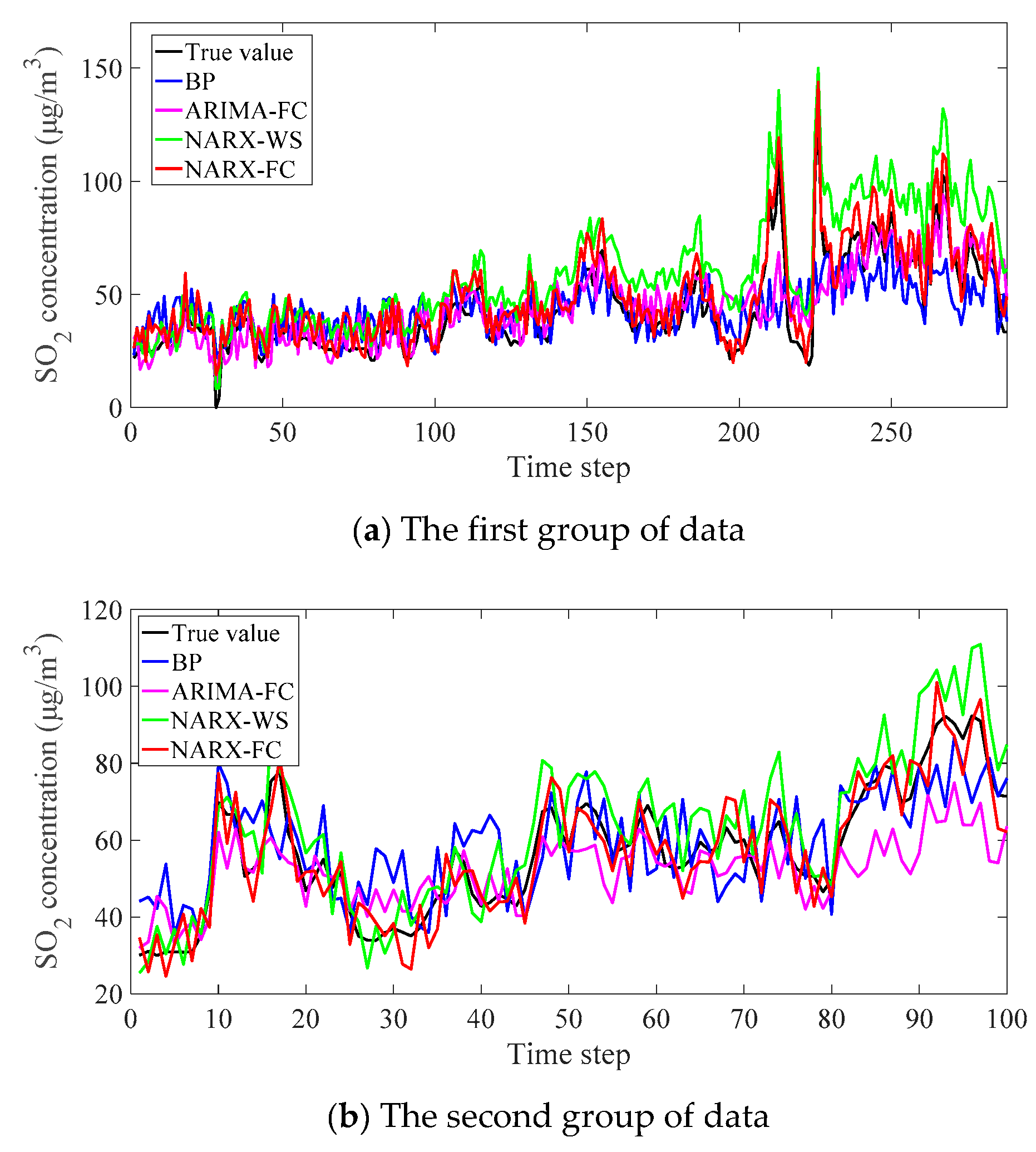
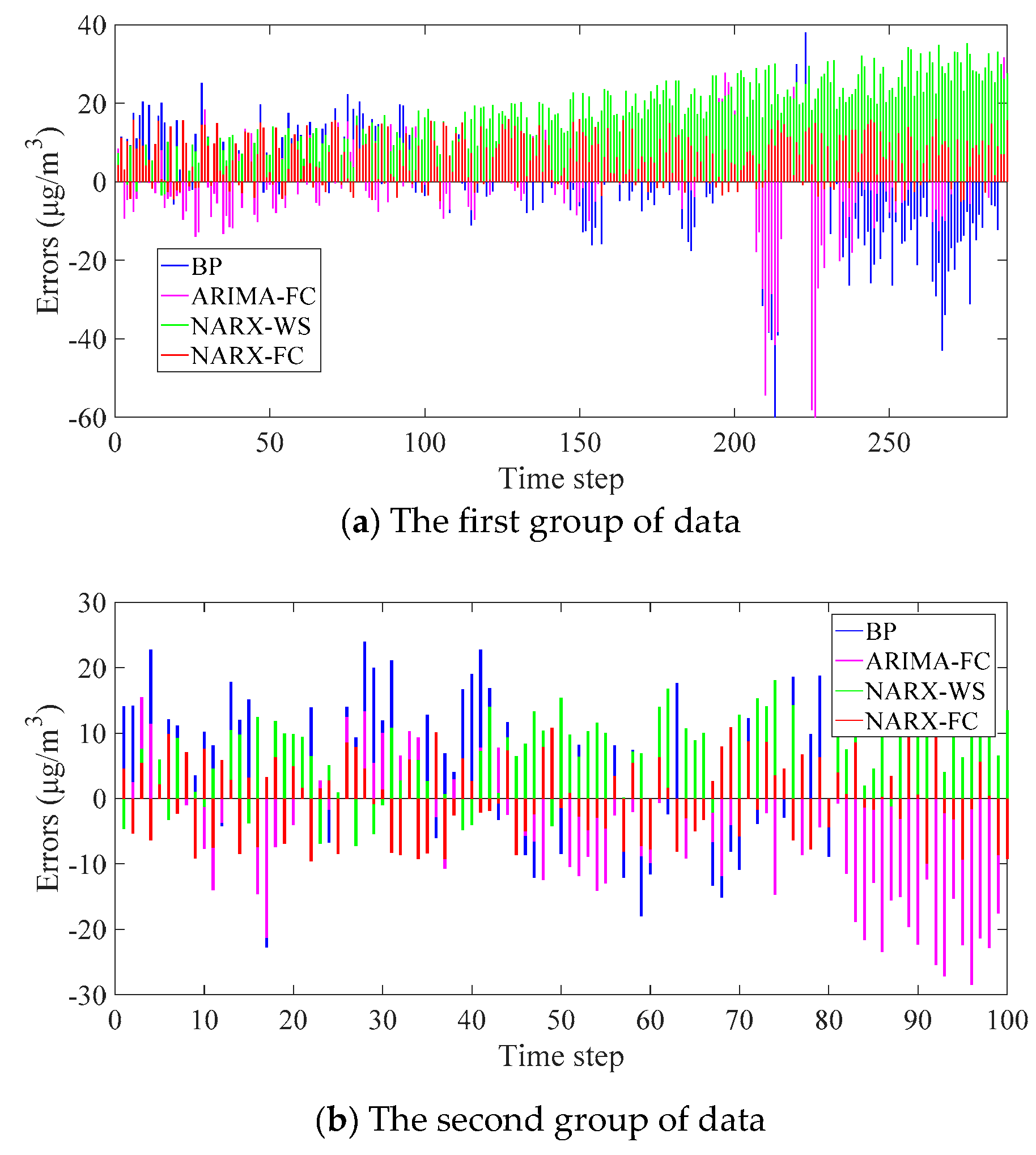
| Data Subsets | Error Indicator | BP | ARIMA-FC | NARX-WS | NARX-FC |
|---|---|---|---|---|---|
| First group | MAE | 10.5835 | 9.0415 | 16.9133 | 7.1388 |
| RMSE | 14.5723 | 12.8278 | 18.9587 | 8.6520 | |
| Second group | MAE | 9.2676 | 8.4514 | 7.3071 | 5.3797 |
| RMSE | 11.2321 | 10.9401 | 8.9681 | 6.1651 |
© 2019 by the authors. Licensee MDPI, Basel, Switzerland. This article is an open access article distributed under the terms and conditions of the Creative Commons Attribution (CC BY) license (http://creativecommons.org/licenses/by/4.0/).
Share and Cite
Bai, Y.-t.; Wang, X.-y.; Sun, Q.; Jin, X.-b.; Wang, X.-k.; Su, T.-l.; Kong, J.-l. Spatio-Temporal Prediction for the Monitoring-Blind Area of Industrial Atmosphere Based on the Fusion Network. Int. J. Environ. Res. Public Health 2019, 16, 3788. https://0-doi-org.brum.beds.ac.uk/10.3390/ijerph16203788
Bai Y-t, Wang X-y, Sun Q, Jin X-b, Wang X-k, Su T-l, Kong J-l. Spatio-Temporal Prediction for the Monitoring-Blind Area of Industrial Atmosphere Based on the Fusion Network. International Journal of Environmental Research and Public Health. 2019; 16(20):3788. https://0-doi-org.brum.beds.ac.uk/10.3390/ijerph16203788
Chicago/Turabian StyleBai, Yu-ting, Xiao-yi Wang, Qian Sun, Xue-bo Jin, Xiao-kai Wang, Ting-li Su, and Jian-lei Kong. 2019. "Spatio-Temporal Prediction for the Monitoring-Blind Area of Industrial Atmosphere Based on the Fusion Network" International Journal of Environmental Research and Public Health 16, no. 20: 3788. https://0-doi-org.brum.beds.ac.uk/10.3390/ijerph16203788