Article

Statistical Evaluation of Radiofrequency Exposure during Magnetic Resonant Imaging: Application of Whole-Body Individual Human Model and Body Motion in the Coil

1
Division of Medical and Biological Measurement, National Institute of Metrology, Beijing 100029, China
2
School of Biomedical Engineering, Dalian University of Technology, Dalian 116024, China
3
China Academy of Information and Communications Technology, Beijing 100191, China
4
XGY Medical Equipment Co. Ltd., Ningbo 315400, China
5
Ningbo Tongde Medical Equipment Technology Co. Ltd., Ningbo 315000, China
*
Authors to whom correspondence should be addressed.
The authors contributed equally to the study.
Int. J. Environ. Res. Public Health 2019, 16(6), 1069; https://0-doi-org.brum.beds.ac.uk/10.3390/ijerph16061069
Submission received: 28 December 2018 / Revised: 20 March 2019 / Accepted: 21 March 2019 / Published: 25 March 2019

Abstract

:
The accurate estimation of patient’s exposure to the radiofrequency (RF) electromagnetic field of magnetic resonance imaging (MRI) significantly depends on a precise individual anatomical model. In the study, we investigated the applicability of an efficient whole-body individual modelling method for the assessment of MRI RF exposure. The individual modelling method included a deformable human model and tissue simplification techniques. Besides its remarkable efficiency, this approach utilized only a low specific absorption rate (SAR) sequence or even no MRI scan to generate the whole-body individual model. Therefore, it substantially reduced the risk of RF exposure. The dosimetric difference of the individual modelling method was evaluated using the manually segmented human models. In addition, stochastic dosimetry using a surrogate model by polynomial chaos presented SAR variability due to body misalignment and tilt in the coil, which were frequently occurred in the practical scan. In conclusion, the dosimetric equivalence of the individual models was validated by both deterministic and stochastic dosimetry. The proposed individual modelling method allowed the physicians to quantify the patient-specific SAR while the statistical results enabled them to comprehensively weigh over the exposure risk and get the benefit of imaging enhancement by using the high-intensity scanners or the high-SAR sequences.

1. Introduction

Magnetic resonance imaging (MRI) is a widely used and powerful imaging technique for non-invasive clinical diagnosis [1]. In order to excite the detectable MR signals, its scanner typically includes a transmit (Tx) coil to generate a homogeneous circular polarized B1 field [2]. The induced eddy current is the primary radiofrequency (RF) absorption mechanism of the B1 field exposure, which will result in tissue heating. As a consequence, RF electromagnetic field (EMF) power deposition and the resulting tissue heating should be carefully managed, which becomes an important safety concern in sequence and coil design. Specific absorption rate (SAR) has been used to prevent excessive exposure [3]. International Electrotechnical Commission [4] defined the SAR averaged over whole body (wbSAR), over the head (hdSAR), over the partial body, and the peak SAR averaging over 10 g tissue (pSAR10g) as the limits.
For MRI exposure, overestimation for SAR may improperly restrict clinical MRI scans with new sequences, whereas underestimation of SAR can lead to tissue heating and thermal injury. Accurate SAR predication is critical for ensuring regulatory compliance, while completely exploiting the potential of the MRI system because of optimizing the imaging quality by repetitive scans or increasing the emissions in sequence resulted in higher SAR [5].
At present, SAR is usually non-invasively characterized using numerical simulations. A representation of the patient-specific SAR depends on the coil model and the individual model [6]. To date, accurate individual models are usually reconstructed using MRI [7]. In this case, the high-intensity scanner and high-SAR sequence were frequently applied to present the precise anatomical details. Non-rigid registration using the brain [6] and breast model libraries [8], tissue simplification [9,10], or body truncation [5] techniques allowed generating an individual human model by a low-intensity scan with an SAR-reduced sequence [6,11].
Nevertheless, the abovementioned methods either focused on partial body modelling or obscured the anatomical and physiological details which may influence the SAR. In this case, it is desirable to derive the a priori knowledge for the measurable anthropometric parameters (e.g., profile, height and weight) and the internal anatomy. However, the relationship was too complicated to be quantified [12].
Our recently developed deformable Chinese phantom [13,14] may help resolve the dilemma. In these studies, deformable human torso and head phantoms were constructed by learning the inter-subject anatomical variation from a segmented computed tomography (CT) dataset of healthy Chinese adults. To match the personal anatomy, the deformable phantoms were registered to individual body surface, which can be obtained by a 3-D surface optical scan. As a consequence, the individual model can be generated in less than 10 minutes using a personal computer and it is free of an MRI scan. The applicability of this kind of model in patient-specific SAR assessment could be promising but the resulting errors should be investigated, and some further work needs to be conducted to finalize the whole-body modelling (e.g., the limbs cannot be generated by the method because the CT dataset did not include this part).
Positioning of the patient in the scanner usually involves random misalignment, which is inevitable in clinical scans [15]. Among the three directions, the shift along the long-axis of the coil (Z-axis) was roughly controlled compared to the other directions which were practically confined by padding or spacers. The Z-axis alignment was based on several body landmarks (e.g., shoulder, groin) and the shift could introduce substantial SAR change [16]. Besides, the body tilt was frequently observed due to the inaccuracy in coil installation (leading to a relative rotation between the excitation port and the body) or the slight motion of the patient. The extent of variation has been evaluated for the Z-axis shift mainly using the deterministic method [5,16] whilst no report was available for the body tilt. In comparison, the stochastic approach addressed the SAR variability based on the probability distribution of the input variables [12,17,18,19,20]. The statistical results would be appropriate for MRI exposure assessment because clinical physicians could manage SAR at different risk levels when weighing over the benefit from the SAR-enhanced sequence.
In this work, we proposed a whole-body individual modelling method, including deformable phantom and tissue simplification, to evaluate the patient-specific exposure to B1 field of MRI. For this purpose, a commercial Tx coil was numerically reconstructed and verified by measurement. The whole-body individual model could be efficiently generated with high accuracy and contained 37 (male) and 34 (female) different tissues. Stochastic dosimetry was conducted using a surrogate model [21] constructed by polynomial chaos [22]. The exposure variability due to the Z-axis misalignment and tilt of the subject was quantified. Both the deterministic and stochastic results validated the application of the individual modelling technique in evaluating the RF exposure of Tx coil. The statistical results fitted well for the need for exposure risk management in MRIs. The procedures as well as the modelling method can be used for efficient patient-specific SAR during MRI assessment.

2. Materials and Methods

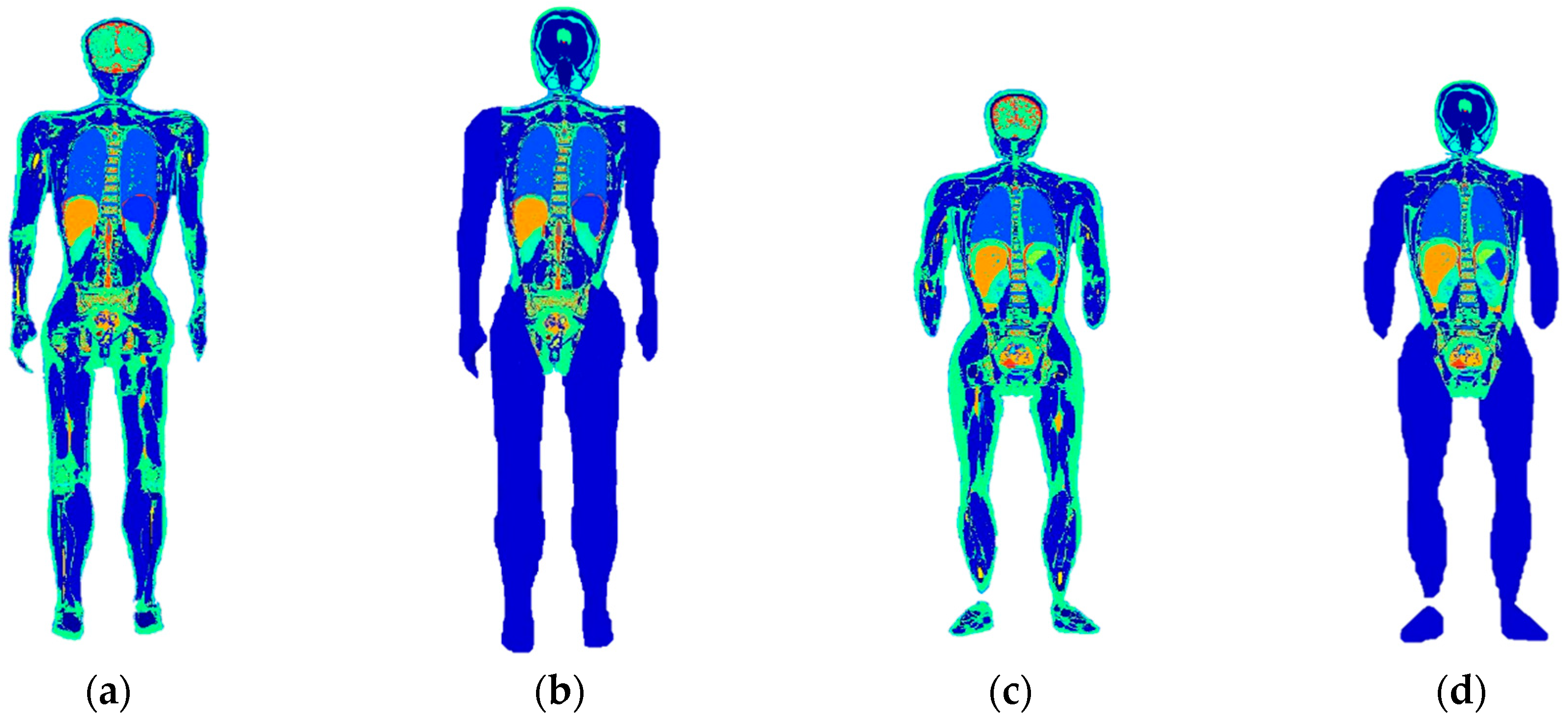
2.1. Whole-Body Individual Modelling

The deformable human phantoms were recently generated for the human torso [13] and head [14] while representing the physical parameters in a given Chinese population. Statistical shape model [23] was used to learn about the inter-subject anatomical variation from a CT dataset containing 79 healthy Chinese, whose tissues were either automatically segmented or mapped using the anatomical templates [24], depending on the specific imaging contrast. To match the personal anatomy for individualized modelling, the deformable phantoms were registered to the individual body profile (can be achieved by an optical scanner) using an active shape model [25]. This was an efficient method (less than 10-min’s calculation on a personal computer) free of MRI scans. However, the abovementioned registration method cannot be applied for limbs because they were not included in the CT database. In the experiments, we assumed that the limbs were homogeneous with muscle.
In order to validate the proposed modelling method, we selected the Chinese adult female and male models [26] as references. The models were manually segmented and reconstructed from cryo-section slices by 10 anatomical experts at the resolution of 1 mm3. Rigorous quality control has been ensured in the process [27]. They were assumed to present the individual anatomical structure with high confidence. Their profiles were extracted and used for whole-body individual modelling with the procedures described in the previous paragraph. The human models reconstructed by manual segmentation and by the approach as we introduced in this study are shown in Figure 1.
The tissues in the abovementioned models are listed in Table 1. The number of the tissues for the male models was 66 (manually segmented model) and 37 (individualized model). As for the female models, the manually segmented model contained 62 tissues, while the individualized model had 34 tissues.

2.2. Computational Method

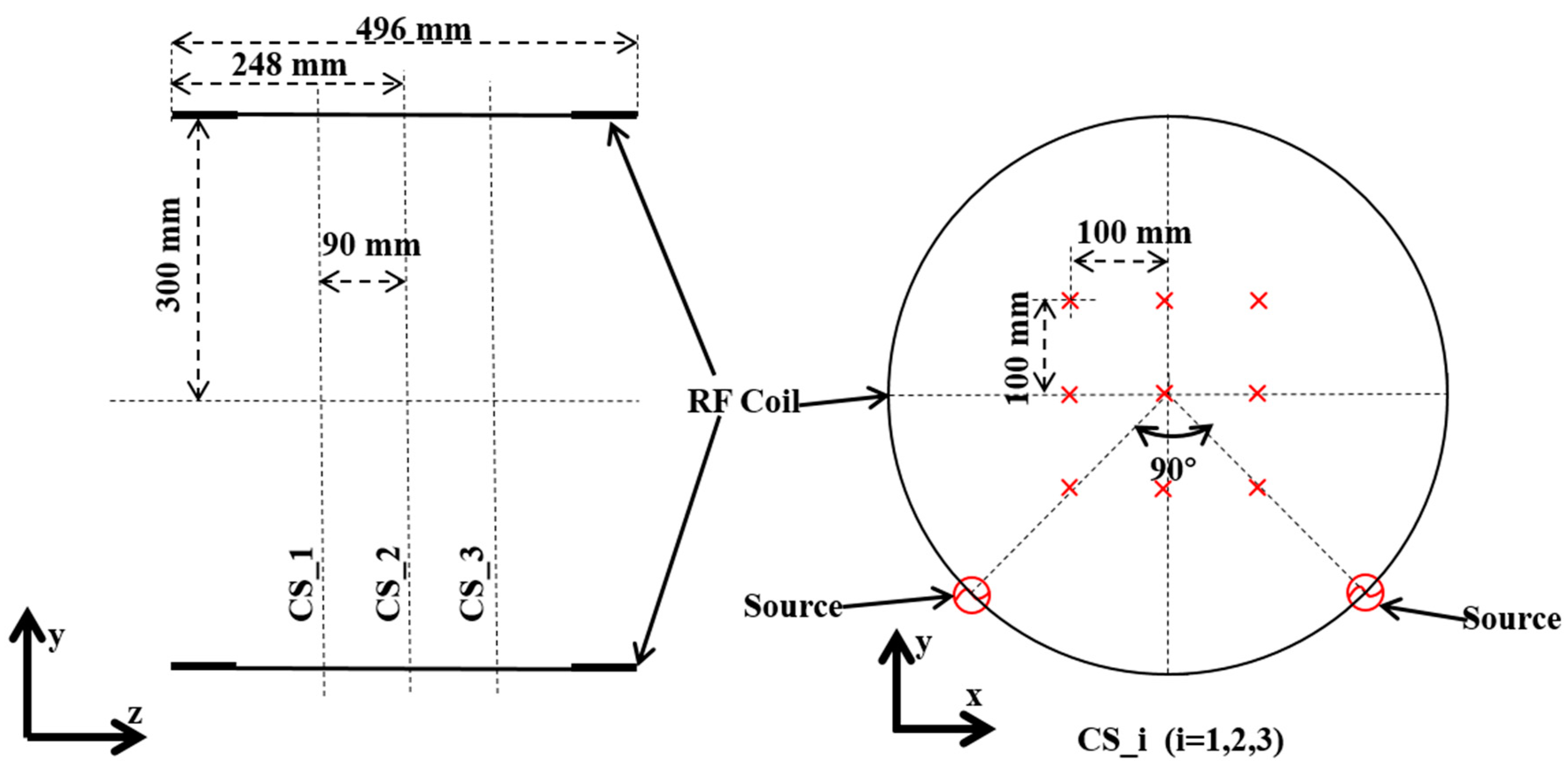
2.2.1. Deterministic Simulations

Finite-Difference Time-Domain (FDTD) is commonly used for electromagnetic dosimetry [28]. It works in time domain and is capable of solving the time response of a pulse for heterogeneous tissues. In contrast, the method has difficulty to handle the large-scale problem with a fine resolution, which introduces huge memory cost. In addition, the steady-state solutions are obtained by simulating the whole transient time response of the system and this can result in very long simulation times for strong resonators. To overcome the drawbacks, we used the equivalent source [29] and the adaptive voxels [28] to reduce the simulation volume.
Taking the coil used in the experiments for an example, a generic 1.5 T 16-rung Tx coil fabricated by XGY Medical Equipment Co. Ltd, (Ningbo, Zhejiang, China) was used in the study (Figure 2a). The dimensions of the coil are shown in Figure 2b. The coil model was tuned to 64 MHz by adjusting the between-rung capacitors. By the method, the calculated return loss (S11) was −12.7 dB, close to the measured one (−13.3 dB).
The incident field was obtained for this Tx coil model which was discretized with an adaptive grid schema (496 × 496 × 411 = 101.52 MCells). The result was used as input for the Huygens Box simulations [28] with the anatomical model at a uniform grid resolution of 2 mm3.
All simulations have been performed with SEMCAD V17.2.1 (SPEAG, Zurich, Switzerland). For the approximate 36.8 MVoxel of the entire simulation space for the human model, the calculation time was around 0.5 h per simulation on a hardware accelerated cluster (CPU: 2 × Xeon E5-2630, 2.2 GHz; Memory on board: 256 GB; GPU: 2 × NVIDIA Tesla K40c with 24 GB memory in total). Two quadrature feeding ports were located in the upper-end ring. The numerical simulations were performed in a multi-port simulation mode with E-field data superimposed from the results of the two quadrature feeds. Frequency-dependent dielectric properties were adopted from the databases of Gabriel et al. [30] and Hasgall et al. [31]. The values were directly used for the manually segmented models. In contrast, we need to homogenize the dielectric properties of the tissues for the individual models as shown in Table 1. The homogenization was based on the mass as shown in (1):
ε ~ homogenized = i = 1 N ε ~ i m i i = 1 N m i = σ + j ω ε
where, ε ~ homogenized is the complex dielectric properties of the homogenized tissue; ε ~ i and m i denote the complex dielectric properties and mass of the ith tissue contained in the homogenized tissue; σ is the conductivity; and ε′ is the relative permittivity.
The homogenized results are shown in Table 2.
The human models were positioned in the coil with their long axis aligning with the Z-axis of the coil. The middle level of the coil along the Z-axis was aligned to the central heart level of the human models. This was defined as the standard position for the human model in the coil. To evaluate the variability due to the body motion in the coil, the models can move along the Z-axis for ±10 cm and rotate for ±5°. The configurations are shown in Figure 3. The minimum distance between the arms and the coil was 7 cm for the adult female model and 6 cm for the adult male model.

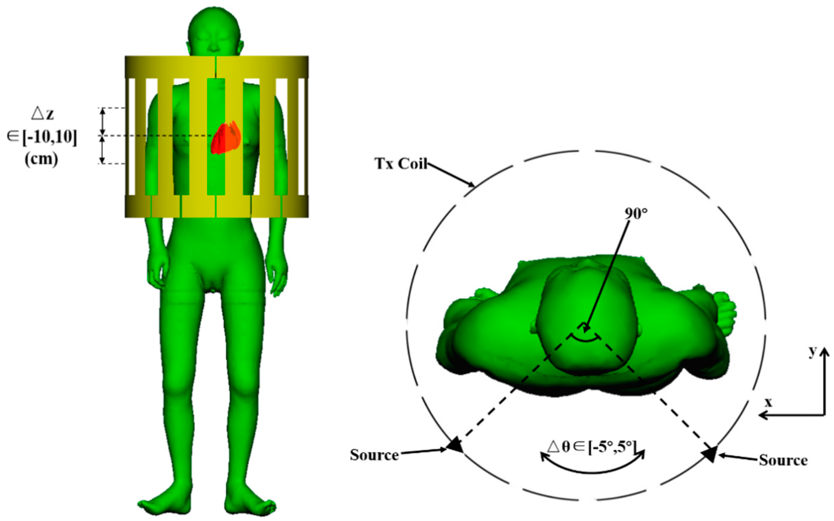
2.2.2. Stochastic Dosimetry on Z-Axis Shift and Body Tilt

Stochastic methods are capable of evaluating the exposure in realistic conditions [12]. The system output (i.e., the dosimetric quantity under assessment) is acquired on the basis of a few observations of the system output obtained by deterministic simulations. Recently, spectral method, in particular, polynomial chaos (PC), has been widely used in the variability analysis of bioelectromagnetic dosimetry at a lower computational cost [32]. It approximates the system outputs by a surrogate model using a series of orthogonal polynomial basis ( ψ ( X ) ) as in (2).
S A R = M ( X ) = 0 P 1 a j ψ j ( X ) + e
where X is the random input vectors made of the variables under assessment (Z-axis shift and body tilt in our case), ψ j ( X ) are the polynomials from ψ ( X ) , a j are the coefficients to be estimated, and e is the truncation error. P is the size of the polynomial basis and is calculated as (3):
P = ( K + p p ) = C p + K p
where p is the maximum order of ψ ( X ) and K is the number of input variables. If the input variables are independent, ψ(X) can be represented as (4):
ψ ( X ) = j = 1 K π α j ( x j ) = π α 1 ( x 1 ) × . . × π α K ( x K )
where π α j is a family of polynomial orthogonals with respect to the probability density function (PDF) of each input variable x i , and α j , 1 j K represents the maximum degree of the polynomials in π α j [22,33]. Practically, the probability density of the Z-axis shift and rotation were assumed to follow Gaussian distribution, respectively. Therefore, Hermite polynomials were selected.
Usually, Least Angle Regression (LAR) algorithm [34] is used to estimate the coefficient of PC. This algorithm is based on least-square regression with respect to the series of observations of the system output S A R o = { s a r 1 , s a r 2 , , s a r N } . The validation of the surrogate model was based on a leave-one-out cross validation approach (LOOCV) [35]. This technique can reduce the size of the experimental design. By this way, the observation set, obtained with deterministic dosimetry from the experimental design to an experimental design X o = { x 1 , x 2 , , x N } , is recursively divided into two subsets, the learning set to build the surrogate model and the testing set to calculate the resultant errors. The best PC expansion among the ones generated by LAR is then chosen through LOOCVs, using the corrected relative leave-one-out error ( ε LOO [36]. ε LOO is based on the estimation of the mean square error of the model as shown in (5)
ε LOO = 1 N i = 1 N ( M ^ J ( x i ) M ( x i ) ) 2
where, M ^ J is the model based on N-1 simulated SAR values, { s a r 1 , s a r 2 , , s a r N } { s a r J } .
The PC procedure should be repeated by increasing the size N of the experimental design and changing the maximum degree p of the polynomials ψ(X) until the achieved error is below a given threshold 1 Q 2 = ε L O O σ s a r 2 , where σ s a r 2 is the variance of the output SAR values.
We used Latin Hypercube Sampling (LHS, [37]) to generate the input variable vectors. The LHS technique is a multidimensional version of the stratified sampling method. It has the advantage of generating a set of samples that more precisely reflect and explore all the distributions with substantially fewer samples.

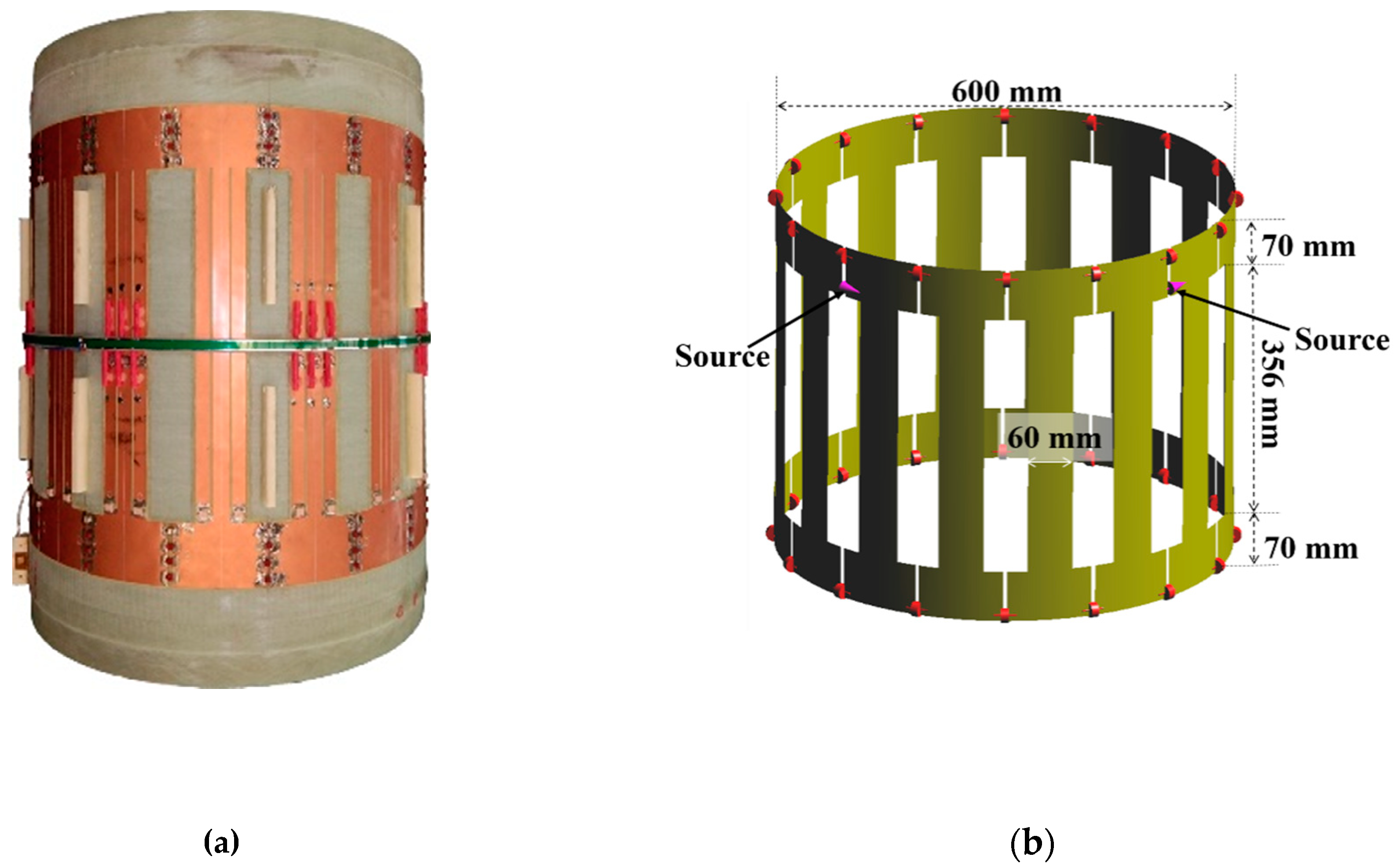
2.3. E-Field Measurement in the Empty Coil

To confirm the field distribution by numerical modelling of the coil, we measured the E-field strength on 27 points distributing on three cross-sections perpendicular to the Z-axis of the coil using E-field probe (ER3DV6) and H-field probe (H3DV7) with Easy4MRI system (SPEAG, Zurich, Switzerland). The measurement configuration is shown in Figure 4. We performed the E-field measurement with the sequence of the modulated rectangular pulse for comparison. The validation measurement and simulation were conducted in the empty coil.

3. Results

3.1. Whole-Body Individual Models

We compared the total mass of the different models as well as some major tissues/organs in the human models in Table 3. Their registration accuracy is also compared in the table.
The deviation of mass for the entire body, skin, fat, muscle, bones, and brain were less than 10%. The deviation of mass for the major organs was generally less than 20% but the registration error (Dice) was rather large, ranging from 61% to 81%.

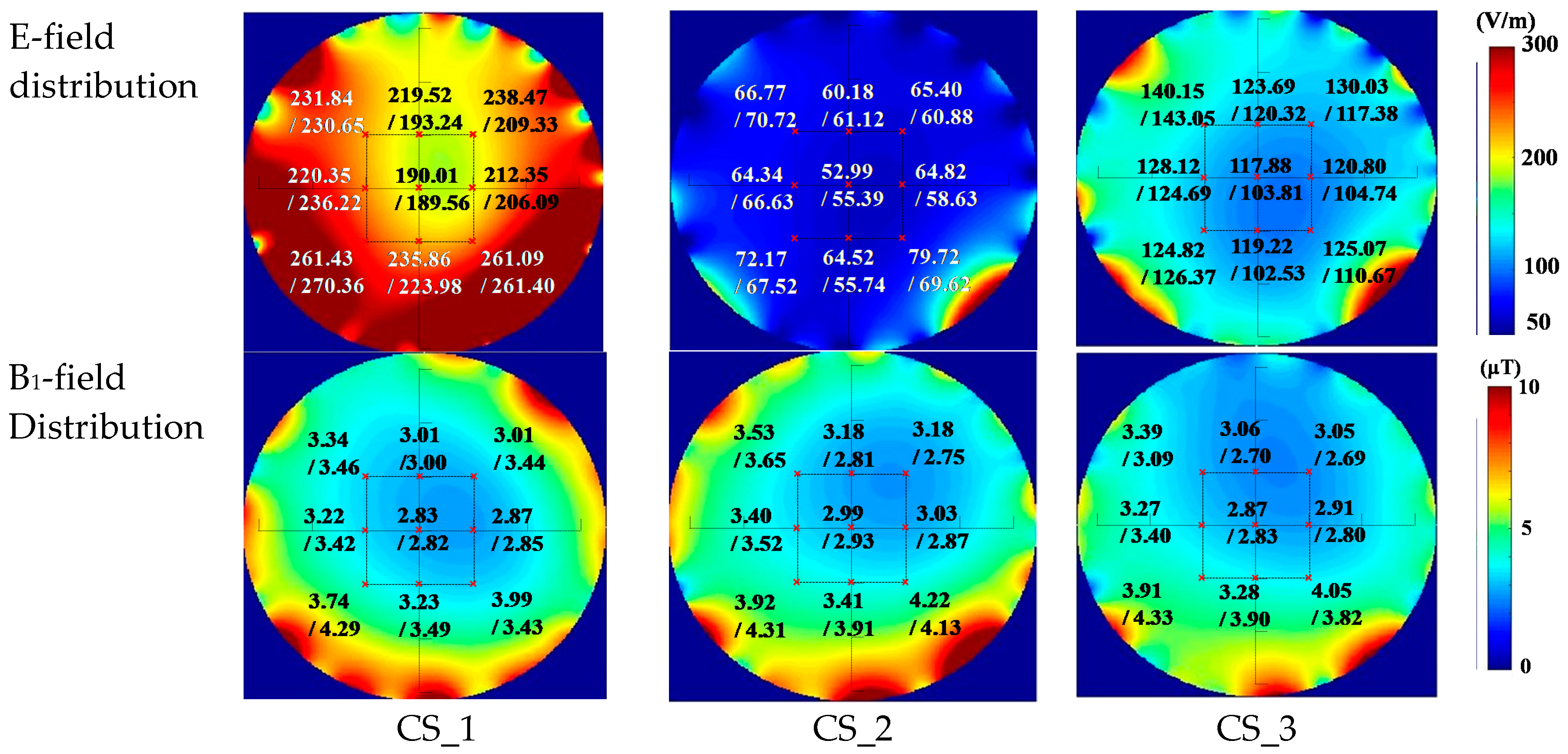
3.2. Comparison for the Simulation and the Measurement Results in the Empty Coil

The calculated and the measured E and B1 field results are shown in Figure 5.
The incident power was not identical for the simulation and measurement due to the inaccuracy in modelling. The discrepancy could be adjusted and compensated in simulations. In fact, the similarity of field distribution was a much more important factor. The mean deviation of the amplitude on these points was 6.13%, with a standard deviation of 3.92%. The maximum deviation was 14.42%.

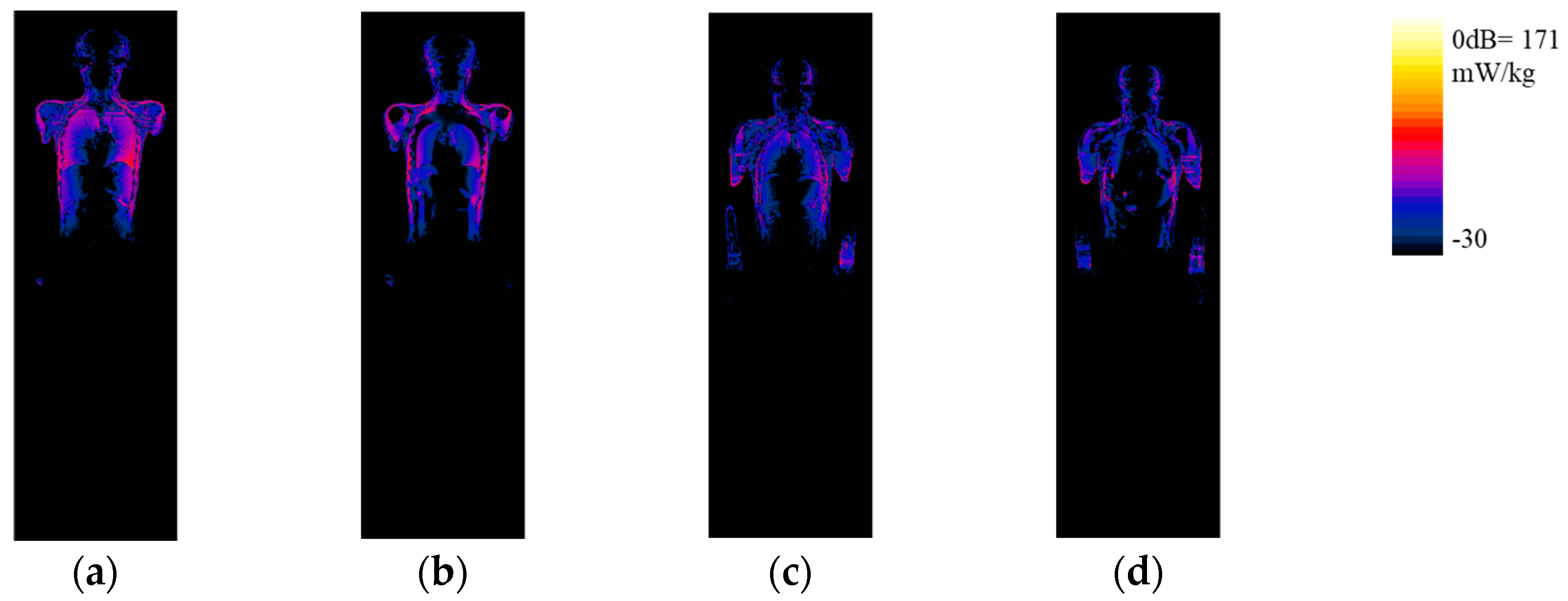
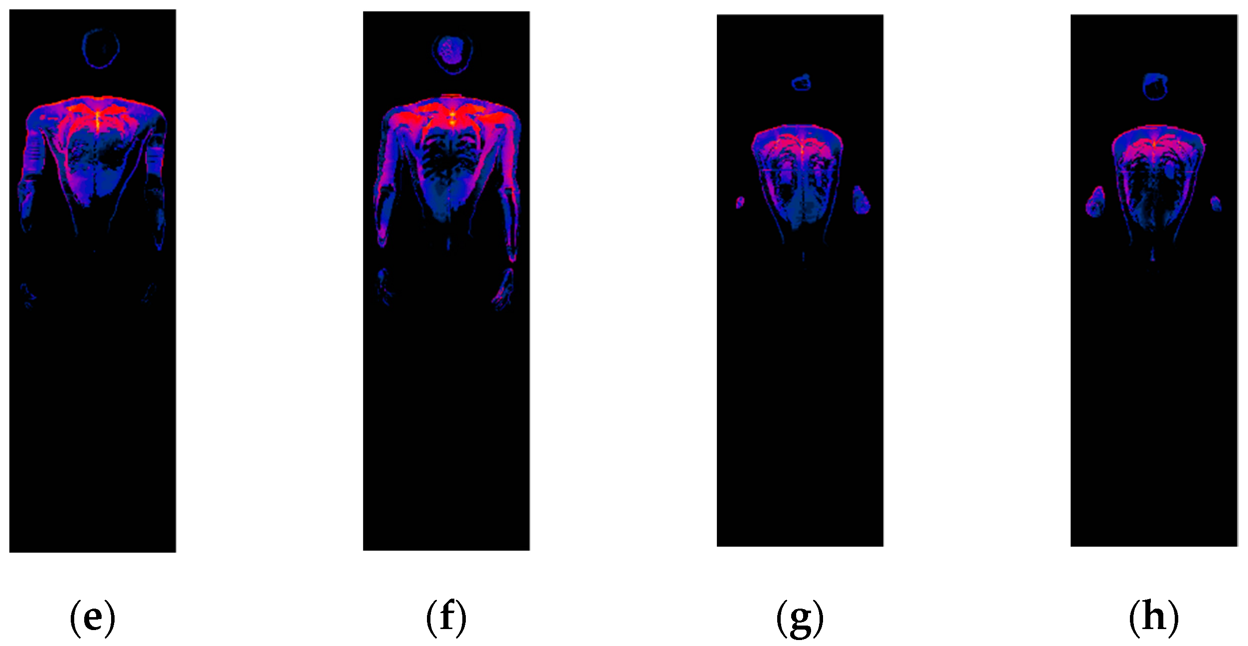
3.3. Deterministic Results

The SAR distribution on the coronal slices is shown in Figure 6.
wbSAR and pSAR10g for the standard position are shown in Table 4.
The difference for wbSAR between the manually segmented models and the individual models was below 4% whilst the difference for pSAR10g between these models was less than 10%. The location of pSAR10g was very close between the manually segmented and the individual models.

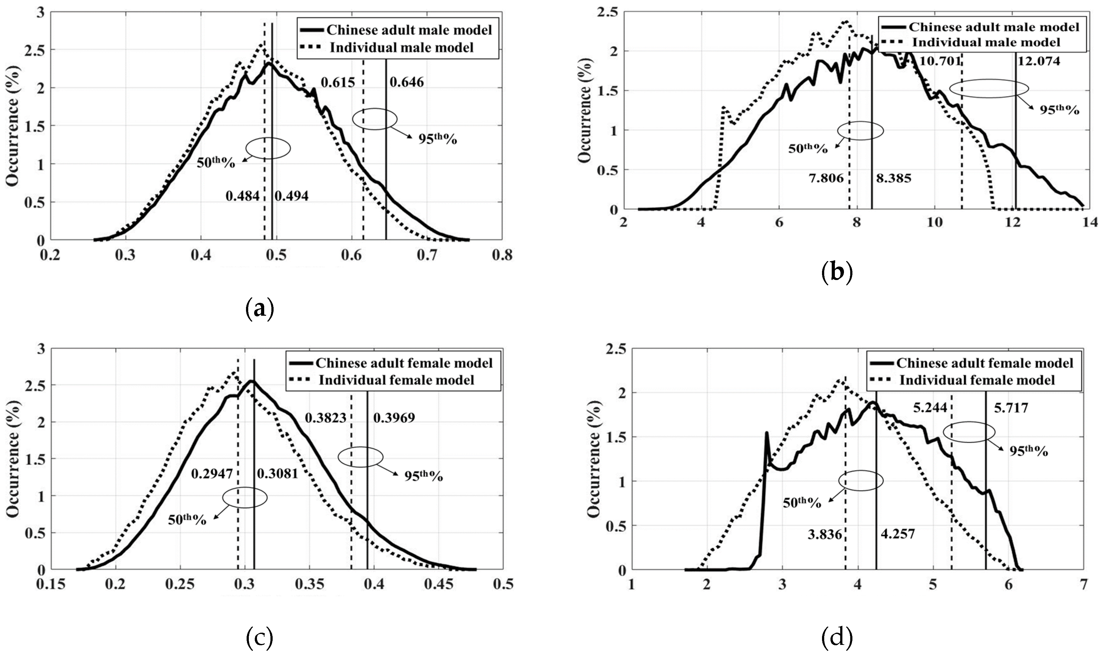
3.4. Statistical Results

By LOOCV, a total of 100 experiments introduced the errors of less than 2% for the wbSAR results (1.12% for the Chinese adult male model, 0.2% for the individual male model, 0.5% for the Chinese adult female model, and 0.1% for individual female model). In comparison, the errors were less than 5% in terms of pSAR10g (4.2% for the Chinese adult male model, 1.2% for the individual male model, 4.8% for the Chinese adult female model, and 1.8% for the individual female model).
Based on the obtained surrogate model, the distribution of wbSAR and pSAR10g due to body motion in the coil is plotted in Figure 7.
The results indicated that the individual models yielded similar SAR results even for various percentiles. For example, at the 50th percentile, the deviation for wbSAR from the male models is 2.07% and 4.54% for the female models. At the 95th percentile, the deviation is 5.04 % for the male models and 3.82% for the female models. Deviation for pSAR10g ranged from 7% to 13% at the 50th and 95th percentile.

4. Discussion

The models generated by the proposed modelling technique gave satisfactory accuracy of SAR estimation compared to the available fast individual modelling methods which demonstrated a deviation of 10–30% for pSAR10g [6,9]. The advantage of accurate SAR representation could be attributed to the anatomical details preserved by the proposed modelling technique. As known, the tissue distribution is essential to the local SAR. In total, more than 30 different tissues/organs were included in the individual model, which thus benefited for an accurate local SAR estimation. Another advantage of the proposed methodology is also obvious: The variables could be eventually traced to several anthropometry parameters (e.g., height and weight), which were dosimetrically important. This is a prospective method for individual modelling even without an optical or low-SAR MRI scan.
The proposed modelling technique learned the inter-subject anatomical variation from the medical image dataset consisting of 79 healthy Chinese individuals (41 males and 38 females). The representation of the database could be enhanced by the inclusion of more subjects. To note, since the CT dataset was from the healthy subjects, the modelling method cannot be directly applied to the subjects with internal abnormalities, e.g., tumors. Another point that underpinned the modelling technique was the representation of the anatomical templates used for the registration of the low-contrast organs. The current templates were created mainly for demonstrative visualization so that the shapes of the organs were stylized with their profiles being significantly smoothed. Although we have achieved good SAR accuracy, the organ’s registration accuracy as well as the SAR results could be potentially improved by choosing the confirmed anatomically correct templates. To note, including the individual information from other anatomical datasets, even for partial body, can help refine the deformable models. For example, Li et al. [8] provided a feasible approach to fuse the individual breast to the whole-body model.
The limbs were simplified with homogeneous muscle due to the lack of the data for this part. Admittedly, change for the tissue composition can modify the wave propagation inside the body. Muscle was selected as the tissue for the limbs because it had a higher conductivity and permittivity compared to fat. Hence, it may indicate that very significant RF power absorption and conservative results were expected. By numerical comparison, the errors for wbSAR, pSAR10g and the locations were usually less than 10%, which was superior to the existing individual modeling methods [6,9]. Moreover, we analyzed the application of the simplification method to the limbs of the Virtual Family models [38]. Very similar results are presented as well (resulting pSAR10g deviation for less than 5% when the hands and the body were separated). The results were consistent with the previous studies indicating the simplification of the heterogeneous whole-body models using muscle–fat–lung tissues [9]. So, we concluded that limbs had much simpler tissue distribution and our simplification would not pose significant errors. Upper limbs have an important influence on the formation of RF loops when the hands contacted the wrist or hip. In practice, an electrical isolation has been recommended to insert between the arms and the torso as well as between the legs to avoid conducting loops [15,39]. Our study used the similar posture and prevented the first hotspots on the contacting parts. The optical scan can obtain the profile of the individual limbs. By this way, the real distance between the arms and the coils was kept. This case was very similar to cerebrospinal fluid (CSF). We cannot identify CSF from the CT dataset although its dielectric properties were very different compared to the other brain tissues. However, from Table 4, we found that the simplification resulted in less than 5% (in terms of errors of hdSAR) for the simulations.
The results demonstrated the SAR equivalence between the individual models and referenced models. Statistical results also demonstrated that the whole-body individual models could represent the SAR variation due to Z-axis misalignment and body tilt. Statistical results on Z-axis misalignment and the body tilt presented the SAR values for various percentiles. The reasonable safety margin rather than an overestimation factor can be determined upon SAR statistics. Setting the SAR limit to various percentiles covered different number of cases. The much more accurate SAR management can be performed and the physician can decide on the application of the novel sequence depending on the expectation of risk.
Two independent factors for body positioning in the coil were studied. Other sources also contributed to SAR variability including the ones from the dielectric properties and coil models. However, it was difficult to simultaneously take them into consideration due to the curse of dimensionality in high-dimensional problems [40]. The possible solutions may include sensitivity analysis and principle component analysis to determine the factors with dosimetric importance. In reality, the physical variables, such as body size and weight, influenced SAR as well. Researchers attempted to characterise the relationship so as to estimate the subject-specific exposure dose or to determine the conservative exposure dose for a population. For example, Murbach et al. discussed the relationship between the RF absorption and anatomy, but only using five human models [16]. Shao et al. statistically discussed the SAR variability due to the variation of the head volume using the unscented transform method [12]. In their work, the different head models were simply scaled from the head model of Duke [7], and the anatomical validity of the derived models was not addressed. By our method, the individual models were generated and, its resultant SAR difference was demonstrated to be less than 5% (wbSAR) and 10% (pSAR10g). So, we assumed that the individual models well-represented the reference models. Then, we focused our research on variability analysis for the body motion in the coil. In effect, the proposed modeling method can generate the human models representing some pre-defined physical and anatomical features, which is essential for statically evaluating the dosimetric results over a specific population. This is another important issue in MRI RF exposure assessment and we will discuss it in future studies.
The uncertainty for assessing the patient–subject SAR has multiple contributors in addition to human modelling. The model of the Tx coil and the numerical method are also important for accurate SAR prediction. In our experiments, we verified the simulated E-field strength in the empty coil using the measurement data from several points with the RMS value. The purpose was to confirm the Tx model rather than a rigorous uncertainty analysis. In general, the uncertainty for the measurement positioning was about 6–7%. According to the calibration documents, the uncertainty of the probes (with the experimental sequence) was 9.6% (k = 2). The uncertainty was around 50% for coil modelling [41,42]. Different numerical methods contributed approximately 6–15% of the uncertainty [43,44]. The information could be referred to for uncertainty estimation.
The deformable model was generated based on the dataset from the Chinese population. A similar method could be applied to other ethnicities when the relevant dataset is available. The body coil was a common commercial product without special optimization. The individual modelling did not use the tissue cluster based on the dielectric similarity [9], thus it is not frequency dependent. Therefore, the methodology as well as the results could be expected to be applied to the coils working at other Larmor frequencies.
In the study, we removed the RF shield of the coil. The simplification was to facilitate the experiments for probe positioning as well as numerical modelling. The purpose of the study was to investigate the applicability of the human modelling method to the evaluation of the individual MRI RF exposure. The MRI coil model presented in the study acted as a source for exposure. Therefore, the detailed structure was not an influential factor on the conclusion. In practice, researchers can adopt any commercial coil in analysis.

5. Conclusions

In this study, the efficient and low-SAR method to evaluate the patient-specific SAR during MRI scan was presented. We utilized a deformable atlas to render the individual trunk and head model based on the inter-subject anatomical variation learned from the CT dataset. The tissues in the upper and lower limbs were simplified to muscle. In that case, an optical scan or low-SAR MRI scan to obtain the individual profile was sufficient for an accurate patient–subject SAR evaluation compared with the current methods because a lot of individual anatomical and physical details were preserved. Since misalignment and body tilt were almost inevitable in the clinical scan, we statistically analyzed the dosimetric influence of the two factors. The results demonstrated that the proposed modelling method can yield similar statistical results compared with the reference models. SAR values for different percentiles were given using surrogate models reconstructed by polynomial chaos. The statistical results provided useful information when weighing over the exposure risk and the benefit of an SAR-enhancing coil/sequence.

Author Contributions

Conceptualization, W.L. and T.W.; methodology, H.W.; software, P.Z.; validation, C.L., J.S. and S.X.; formal analysis, P.L.; investigation, P.Z.; resources, H.W.; data curation, S.X.; writing—original draft preparation, C.L.; writing—review and editing, T.W.; visualization, Z.C.; supervision, T.W.; project administration, P.Z.; funding acquisition, W.L. and T.W.

Funding

This research was funded by National Key Technology R&D Program of China, grant number 2016YFF0201004, Science Foundations of National Institute of Metrology, grant number 32-AKY1811, National Key Basic Research Project, grant number 2011CB503705, National Natural Science Foundation Project, grant number 61371187 and 61671158 and National Science and Technology Major Project, grant number 2018ZX100301.

Conflicts of Interest

The authors declare no conflict of interest.

References

  1. McRobbie, D.W.; Moore, E.A.; Graves, M.J.; Prince, M.R. MRI from Picture to Proton; Cambridge University Press: Cambridge, UK, 2017. [Google Scholar]
  2. Chen, X.; Steckner, M. Electromagnetic computation and modelling in MRI. Med. Phys. 2017, 44, 1186–1203. [Google Scholar] [CrossRef]
  3. Hand, J.W. Modelling the interaction of electromagnetic fields (10 MHz-10 GHz) with the human body: Methods and applications. Phys. Med. Biol. 2008, 53, R243–R286. [Google Scholar] [CrossRef] [PubMed]
  4. International Electrotechnical Commission. International standard, Medical Equipment IEC 60601-2-33: Particular Requirements for the Safety of Magnetic Resonance Equipment, 3rd ed.; IEC: Geneva, Switzerland, 2010. [Google Scholar]
  5. Wolf, S.; Diehl, D.; Gebhardt, M.; Mallow, J.; Speck, O. SAR simulations for high-field MRI: How much detail, effort, and accuracy is needed? Magn. Reson. Med. 2013, 69, 1157–1168. [Google Scholar] [CrossRef] [PubMed]
  6. Jin, J.; Liu, F.; Weber, E.; Crozier, S. Improving SAR estimations in MRI using subject-specific models. Phys. Med. Biol. 2012, 57, 8153–8171. [Google Scholar] [CrossRef] [PubMed]
  7. Gosselin, M.C.; Neufeld, E.; Moser, H.; Huber, E.; Farcito, S.; Gerber, L.; Jedensjö, M.; Hilber, I.; Gennaro, F.D.; Lloyd, B.; et al. Development of a new generation of high-resolution anatomical models for medical device evaluation: The Virtual Population 3.0. Phys. Med. Biol. 2014, 59, 5287–5303. [Google Scholar] [CrossRef]
  8. Li, X.; Rispoli, J.V. Toward 7T breast MRI clinical study: Safety assessment using simulation of heterogeneous breast models in RF exposure. Magn. Reson. Med. 2019, 81, 1307–1321. [Google Scholar] [CrossRef] [PubMed]
  9. Homann, H.; Börnert, P.; Eggers, H.; Nehrke, K.; Dössel, O.; Graesslin, I. Toward individualized SAR models and in vivo validation. Magn. Reson. Med. 2011, 66, 1767–1776. [Google Scholar] [CrossRef] [PubMed]
  10. Wu, T.; Shao, Q.; Yang, L. Simplified segmented human models for whole body and localised SAR evaluation of 20 MHz to 6 GHz electromagnetic field exposures. Radiat. Prot. Dosim. 2012, 153, 266–272. [Google Scholar] [CrossRef]
  11. Li, C.; Chen, Z.; Yang, L.; Lv, B.; Liu, J.; Varsier, N.; Hadjem, A. Generation of infant anatomical models for evaluating electromagnetic field exposures. Bioelectromagnetics 2015, 36, 10–26. [Google Scholar] [CrossRef] [PubMed]
  12. Shao, Y.; Zeng, P.; Wang, S. Statistical simulation of SAR variability with geometric and tissue property changes by using the unscented transform. Magn. Reson. Med. 2015, 73, 2357–2362. [Google Scholar] [CrossRef]
  13. Wang, H.; Sun, X.B.; Wu, T.N.; Li, C.S.; Chen, Z.H.; Liao, M.Y.; Li, M.C.; Yan, W.; Huang, H.; Yang, J.; et al. Deformable torso phantoms of Chinese adults for personalized anatomy modelling. J. Anat. 2018, 233, 121–134. [Google Scholar] [CrossRef] [PubMed]
  14. Chen, Z.F.; Qiu, T.S.; Huo, L.; Yu, L.J.; Shi, H.C.; Zhang, Y.J.; Wang, H.K. Deformable Head Atlas of Chinese Adults Incorporating Inter-Subject Anatomical Variations. IEEE Access 2018, 6, 51392–51400. [Google Scholar] [CrossRef]
  15. Murbach, M.; Cabot, E.; Neufeld, E.; Gosselin, M.C.; Christ, A.; Kuster, N. Local SAR enhancements in anatomically correct children and adult models as a function of position within 1.5 T MR body coil. Prog. Biophys. Mol. Biol. 2011, 107, 428–433. [Google Scholar] [CrossRef] [PubMed]
  16. Murbach, M.; Neufeld, E.; Kainz, W.; Pruessmann, K.P.; Kuster, N. Whole-body and local RF absorption in human models as a function of anatomy and position within 1.5 T MR body coil. Magn. Reson. Med. 2014, 71, 839–845. [Google Scholar] [CrossRef] [PubMed]
  17. Roman, G.; Scorretti, R.; Sabariego, R.V.; Geuzaine, C. Stochastic uncertainty quantification of the eddy current in human body by using polynomial chaos decomposition. IEEE Trans. Magn. 2012, 48, 451–454. [Google Scholar]
  18. Liorni, I.; Parazzini, M.; Fiocchi, S.; Ravazzani, P. Study of the influence of the orientation of a 50-Hz magnetic field on Fetal exposure using polynomial chaos decomposition. Int. J. Environ. Res. Public Health 2015, 12, 5934–5953. [Google Scholar] [CrossRef] [PubMed]
  19. Liorni, I.; Parazzini, M.; Varsier, N.; Hadjem, A.; Ravazzani, P.; Wiart, J. Exposure assessment of one-year-old child to 3G tablet in uplink mode and to 3G femtocell in downlink mode using polynomial chaos decomposition. Phys. Med. Biol. 2016, 61, 3237–3257. [Google Scholar] [CrossRef] [PubMed]
  20. Ghanmi, A.; Varsier, N.; Hadjem, A.; Conil, E.; Picon, O.; Wiart, J. Analysis of the influence of handset phone position on RF exposure of brain tissue. Bioelectromagnetics 2014, 35, 568–579. [Google Scholar] [CrossRef]
  21. Kersaudy, P.; Sudret, B.; Varsier, N.; Picon, O.; Wiart, J. A new surrogate modelling technique combining Kriging and polynomial chaos expansions–Application to uncertainty analysis in computational dosimetry. J. Comput. Phys. 2015, 286, 103–117. [Google Scholar] [CrossRef]
  22. Wiener, N. The homogeneous chaos. Am. J. Math. 1938, 60, 897–936. [Google Scholar] [CrossRef]
  23. Heimann, T.; Meinzer, H.P. Statistical shape models for 3D medical image segmentation: A review. Med. Image Anal. 2009, 13, 543–563. [Google Scholar] [CrossRef] [PubMed]
  24. Turbosquid. Male and Female Anatomy Complete Pack (Textured). Available online: https://www.turbosquid.com/3d-models/male-female-anatomy-body-3d-max/602826/ (accessed on 4 April 2018).
  25. Cootes, T.F.; Taylor, C.J.; Cooper, D.H.; Graham, J. Active shape models-their training and application. Comput. Vis. Image Underst. 1995, 61, 38–59. [Google Scholar] [CrossRef]
  26. Wu, T.; Tan, L.; Shao, Q.; Li, Y.; Yang, L.; Zhao, C.; Xie, Y.; Zhang, S. Slice-based supine to standing postured deformation for Chinese anatomical models and the dosimetric results by wide band frequency electromagnetic field exposure: Morphing. Radiat. Prot. Dosim. 2012, 154, 26–30. [Google Scholar] [CrossRef] [PubMed]
  27. Wu, T.N.; Tan, L.W.; Shao, Q.; Zhang, C.; Zhao, C.; Li, Y.; Conil, E.; Hadjem, A.; Wiart, J.; Lu, B. Chinese adult anatomical models and the application in evaluation of RF exposures. Phys. Med. Biol. 2011, 56, 2075–2089. [Google Scholar] [CrossRef] [PubMed]
  28. Allen, T.; Hagness, S.C. Computational Electrodynamics: The Finite-Difference Time-Domain Method; Artech House: Boston, MA, USA; London, UK, 2005. [Google Scholar]
  29. Potter, M.; Bérenger, J.P. A Review of the Total Field/Scattered Field Technique for the FDTD Method. FERMAT 2017, 19, 1–13. [Google Scholar]
  30. Gabriel, S.; Lau, R.W.; Gabriel, C. The dielectric properties of biological tissues: II. Measurements in the frequency range 10 Hz to 20 GHz. Phys. Med. Biol. 1996, 41, 2251–2269. [Google Scholar] [CrossRef] [PubMed]
  31. Hasgall, P.A.; Di Gennaro, F.; Baumgartner, C.; Neufeld, E.; Lloyd, B.; Gosselin, M.C.; Payne, D.; Klingenböck, A.; Kuster, N. IT’IS Database for Thermal and Electromagnetic Parameters of Biological Tissues, version 4.0; IT’IS Foundation: Zurich, Switzerland, 2018. [Google Scholar] [CrossRef]
  32. Wiart, J. Radio-Frequency Human Exposure Assessment: From Deterministic to Stochastic Methods; Wiley-IEEE Press: New York, NY, USA, 2016; pp. 119–155. [Google Scholar]
  33. Xiu, D.; Karniadakis, G.E. The Wiener—Askey polynomial chaos for stochastic differential equations. SIAM J. Sci. Comput. 2002, 24, 619–644. [Google Scholar] [CrossRef]
  34. Efron, B.; Hastie, T.; Johnstone, I.; Tibshirani, R. Least angle regression. Ann. Stat. 2004, 32, 407–499. [Google Scholar]
  35. Stone, M. Cross-validatory choice and assessment of statistical predictions. J. R. Stat. Soc. Ser. B Methodol. 1974, 36, 111–133. [Google Scholar] [CrossRef]
  36. Blatman, G.; Sudret, B. Adaptive sparse polynomial chaos expansion based on least angle regression. J. Comput. Phys. 2011, 230, 2345–2367. [Google Scholar] [CrossRef]
  37. Iman, R.L.; Davenport, J.M.; Zeigler, D.K. Latin Hypercube Sampling (Program User’s Guide); [LHC, in FORTRAN]; Sandia Labs.: Albuquerque, NM, USA, 1980. [Google Scholar]
  38. Christ, A.; Kainz, W.; Hahn, E.G.; Honegger, K.; Zefferer, M.; Neufeld, E.; Rascher, W.; Janka, R.; Bautz, W.; Chen, J.; et al. The Virtual Family-developmentof surface-based anatomical models of two adults and two children for dosimetric simulations. Phys. Med. Biol. 2009, 55, N23–N38. [Google Scholar] [CrossRef] [PubMed]
  39. Shellock, F.G. MRI safety and neuromodulation systems. In Neuromodulation; Academic Press: New York, NY, USA, 2009; pp. 243–281. [Google Scholar]
  40. Verleysen, M.; François, D. The curse of dimensionality in data mining and time series prediction. In International Work-Conference on Artificial Neural Networks; Springer: Berlin/Heidelberg, Germany, 2005; pp. 758–770. [Google Scholar]
  41. Capstick, M.; McRobbie, D.; Hand, J.; Christ, A.; Kühn, S.; Mild, K.H.; Cabot, E.; Li, Y.; Melzer, A.; Papadaki, A.; et al. An Investigation into Occupational Exposure to Electromagnetic Fields for Personnel Working with and Around Medical Magnetic Resonance Imaging Equipment. Report on Project VT/2007/017 of the European Commission Employment. 2008. Available online: http://www.itis.ethz.ch/downloads/VT2007017FinalReportv04.pdf (accessed on 25 March 2019).
  42. Li, B.K.; Liu, F.; Weber, E.; Crozier, S. Hybrid numerical techniques for the modelling of radio frequency coils in MRI. NMR Biomed. Int. J. Dev. Appl. Magn. Reson. In Vivo 2009, 22, 937–951. [Google Scholar]
  43. Kozlov, M.; Turner, R. A comparison of Ansoft HFSS and CST microwave studio simulation software for multi-channel coil design and SAR estimation at 7T MRI. Piers Online 2010, 6, 395–399. [Google Scholar] [CrossRef]
  44. Bottauscio, O.; Chiampi, M.; Hand, J.; Zilberti, L. A GPU computational code for eddy-current problems in voxel-based anatomy. IEEE Trans. Magn. 2015, 51, 1–4. [Google Scholar] [CrossRef]
Figure 1. Human models used in the study: (a) Chinese adult male model by manual segmentation; (b) individualized adult male model; (c) Chinese adult female model by manual segmentation; (d) individualized adult female model.
Ijerph 16 01069 g001
Figure 2. Structure of the MRI Tx coil: (a) Tx coil used in the experiment; (b) CAD model of the coil, the red dot indicates the positions of the capacitors.
Ijerph 16 01069 g002
Figure 3. Positioning of the human models in the coil.
Ijerph 16 01069 g003
Figure 4. Field measurement for the Tx coil. CS_i (i = 1, 2, 3) indicates the three measurement surfaces in the coil, which were separated by 90 mm. “x” indicates the position of the measurement point.
Ijerph 16 01069 g004
Figure 5. The simulated and the measured RMS field values on the three selected slices. The values were presented by “simulated result/ measured result”. The measured points were indicated by red x. The power to the coil was 6 kW (in measurement) and 3.5 kW (in simulation).
Ijerph 16 01069 g005
Figure 6. SAR results for the models at the standard position in the coil. (ad) SAR distribution at the central coronal slice for the manually segmented Chinese adult male model, individual male model, manually segmented Chinese adult female model, and individual female model, respectively; (e,f) SAR distribution at the coronal slice which includes pSAR10g for the manually segmented Chinese adult male model, individual male model, manually segmented Chinese adult female model, and individual female model, respectively. The positions of pSAR10g are indicated in the figures. The results were normalized to a net incident power of 1 W.
Ijerph 16 01069 g006aIjerph 16 01069 g006b
Figure 7. SAR occurrence calculated by surrogate model: (a) wbSAR for the male models; (b) pSAR10g for the male models; (c) wbSAR for the female models; and (d) pSAR10g for the female models.
Ijerph 16 01069 g007
Table 1. Tissues for the different models.
Chinese Adult Male ModelIndividualized Adult Male ModelChinese Adult Female ModelIndividualized Adult Female Model
Aqueous humorEyesAqueous humorEyes
CorneaCornea
Cortex_of_lensCortex_of_lens
ScleraSclera
RetinaRetina
Vitreous_bodyVitreous_body
Lens_nucleusLens_nucleus
IrisIris
Lacrimal_apparatusLacrimal_apparatus
Brain_stemBrainBrain_stemBrain
Cerebral_dura_materCerebral_dura_mater
Cerebral_grey_matterCerebral_grey_matter
Cerebral_white_matterCerebral_white_matter
HippocampusHippocampus
HypophysisHypophysis
HypothalamusHypothalamus
CerebellumCerebellum
Cerebrospinal_fluidCerebrospinal_fluid
CartilageCartilageCartilageCartilage
Large_artery_wallLarge_artery_wall
Large_vein_wallLarge_vein_wall
Laryngeal_cartilagesLaryngeal_cartilages
NerveNerve
Vestibulocochlear_nerveVestibulocochlear_nerve
DiploeSkullDiploeSkull
TeethTeeth
BileBile
BladderBladderBladderBladder
BloodBloodBloodBlood
CholecystCholecyst
Cortical_boneCortical_boneCortical_boneCortical_bone
FatFatFatFat
HeartHeartHeartHeart
Internal_earInternal_earInternal_earInternal_ear
Intervertebral_discIntervertebral_discIntervertebral_discIntervertebral_disc
KidneyKidneyKidneyKidney
Large_intestineIntestinesLarge_intestineIntestines
Enteric_cavityEnteric_cavity
LigamentLigamentLigamentLigament
LiverLiverLiverLiver
LungLungLungLung
Lymph_nodeLymph_nodeLymph_nodeLymph_node
Mammary_glandMammary_gland
Intrinsic_laryngeal_muscleMuscleIntrinsic_laryngeal_muscleMuscle
Muscle_bellyMuscle_belly
TongueTongue
Muscle_tendonMuscle_tendon
NucleusNucleusNucleusNucleus
Optical_nerveOptical_nerveOptical_nerveOptical_nerve
PancreasPancreasPancreasPancreas
Pineal_glandPineal_glandPineal_glandPineal_gland
ProstateProstate
Red_bone_marrowRed_bone_marrowRed_bone_marrowRed_bone_marrow
Salivary_glandSalivary_glandSalivary_glandSalivary_gland
SkinSkinSkinSkin
Spinal_cordSpinal_cordSpinal_cordSpinal_cord
Spinal_dura_materSpinal_dura_materSpinal_dura_materSpinal_dura_mater
SpleenSpleenSpleenSpleen
Spongy_boneSpongy_boneSpongy_boneSpongy_bone
StomachStomachStomachStomach
Stomach lumenStomach lumen
TestisTestis
Thoracic_glandThoracic_gland
ThyroidThyroidThyroidThyroid
TracheaTracheaTracheaTrachea
UreterUreterUreterUreter
VesselVessel
Table 2. Dielectric properties for the homogenized tissues of the individual models.
Homogenized TissuesConductivity (S/m)Relative Permittivity
Eyes1.2470.96
Brain0.6972.35
Cartilage0.6066.76
skull0.1326.38
Muscle0.6972.24
Stomach0.8885.81
Table 3. Comparison for the major tissue/organs of the different models.
TissuesChinese Adult Male Model (kg)Individual Male Model (kg)Weight Deviation (%)Dice 1 (%)Chinese Adult Female Model (kg)Individual Female Model (kg)Weight Deviation (%)Dice (%)
Total weight63.2666.705.44/53.4754.992.84/
Fat21.5423.328.26/17.1018.8110.00/
Muscle22.3724.238.31/16.2316.03−1.20/
Skin3.793.77−0.57/3.143.150.27/
Bones8.429.017.00/5.966.224.36/
Brain1.381.39−1.4981.081.301.26−2.6778.75
Heart0.420.35−17.0069.490.270.3011.1169.98
Kidney0.260.2911.5369.550.220.19−13.6363.83
Liver2.051.84−10.2463.171.171.02−12.8061.76
Lung1.020.90−11.7663.390.930.86−7.7668.87
Spleen0.190.16−15.7961.180.180.14−16.6763.22
Stomach0.760.74−2.6372.320.590.6713.5569.70
1 Dice (%) is calculated by 2 | X Y | | X | + | Y | × 100 % , where X and Y are the voxels of the organ belonging to the manually segmented model and the individual model, respectively.
Table 4. Deterministic simulation results for the models at the standard position in the coil.
Human ModelswbSAR 1Deviation
(%) 2
hdSAR 3Deviation
(%)
pSAR10gDeviation (%)Location of pSAR10g
Manually segmented male model0.48 mW/kg−2.620.27 mW/kg3.208.39 mW/kg−7.55(86, 85, 489)
Individual male model0.47 mW/kg0.28 mW/kg7.76 mW/kg(101, 86, 492)
Manually segmented female model0.31 mW/kg−3.060.21 mW/kg4.534.24 mW/kg−9.09(93, 79, 461)
Individual female model0.30 mW/kg0.22 mW/kg3.85 mW/kg(96, 82, 463)
1 wbSAR is the SAR averaged over the entire body. 2 Deviation is calculated by the difference of the two models divided by the value from the manually segmented model. 3 hdSAR is the SAR averaged over the entire head. The results were normalized to net incident power of 1 W.

