Research on the Decoupling of Water Resources Utilization and Agricultural Economic Development in Gansu Province from the Perspective of Water Footprint

Abstract
:1. Introduction
2. Literature Review
3. Methods and Model
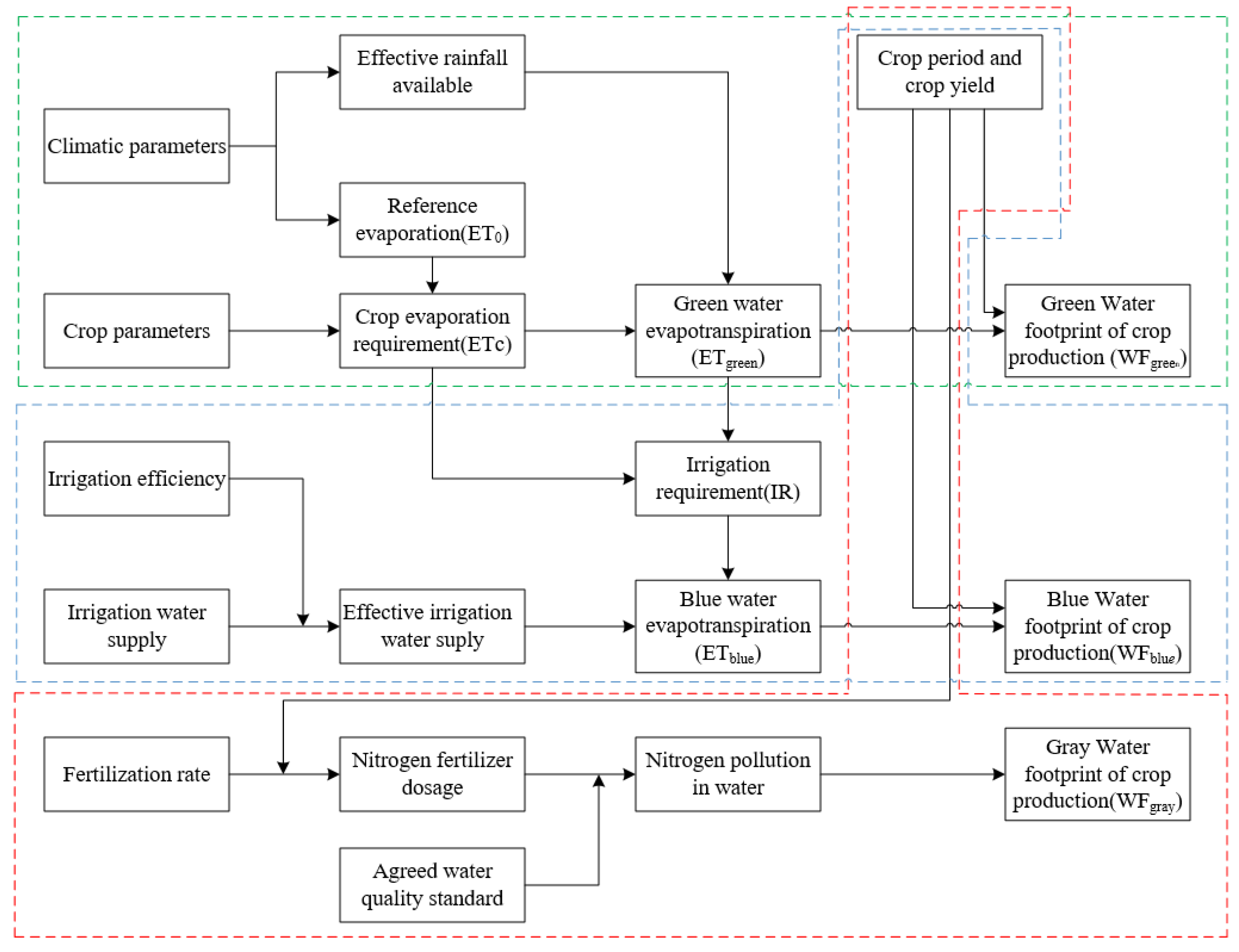
3.1. Water Footprint Evaluation
- (1)
- The blue WF of crop production is mainly represented by irrigation water (IR), which equals to the actual planted area (hm2) multiplied by the irrigation quota (m3 hm−2) per year. The irrigation quota here varies according to the type of crop and rainfall in a year, which entirely depends on the actual situation of crop planting in Gansu Province.
- (2)
- Green water footprint here was represented by effective rainfall or crop evaporation, which can be estimated with the CROPWAT8.0 model:WFgreen = 10 × ETgreen × Awhere ETgreen is green water evapotranspiration (mm); that is the crop evapotranspiration during the growth period (mm). ETc refers to the crop evapotranspiration (mm); Peff is the effective precipitation (mm); A is the plant area of calculated crops (hm2); the factor 10 converts water depth (mm) into water volume per acreage (m3 hm−2). ETc and Peff can be directly calculated by using CROPWAT8.0 model.ETgreen = min (ETc, Peff)ETc was calculated by reference evaporation along with crop factors. The calculation of reference evaporation (ET0) was derived from the latest revised F.A.O. Penman–Monteith method, given by the following relationship [38]:where ET0 is reference evapotranspiration (mm day−1); Rn is net radiation at the crop surface (MJ m−2 day−1); G represents the soil heat flux density (MJ m−2 day−1); T refers to mean daily air temperature at 2 m height (°C); u2 is the wind speed at 2 m height (m s−1); es is the saturation vapor pressure (kPa); ea means actual vapor pressure (kPa); es − ea is the saturation vapor pressure deficit (kPa); ∆ means slope vapor pressure curve (kPa °C−1); γ is the psychrometric constant (kPa °C−1), and Kc means crop factors.ETc = ET0 × Kc
- (3)
- The gray water used to assimilate nitrogen contamination from fertilizers is evaluated as gray water consumption. The WFgray of growing a crop can be calculated as follows (Hoekstra et al. (2009) [31]):where a is the leaching rate of N fertilizer (%); AR is the amount of N fertilizer used per unit area of a crop (kg hm−1); Cmax means the maximum permissible concentration of nitrogen per unit volume of water (kg m−3), under current environmental water quality standards; Cnat represents the natural concentration of nitrogen per unit volume of water (kg m−3), and Y refers to the crop yield (t hm−1).
3.2. LMDI Factor Decomposition Model
3.3. Tapio Decoupling Index
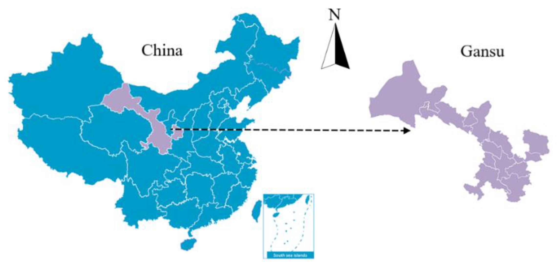
3.4. Data Source and Description
4. Empirical Study
4.1. Descriptive Statistical Analysis
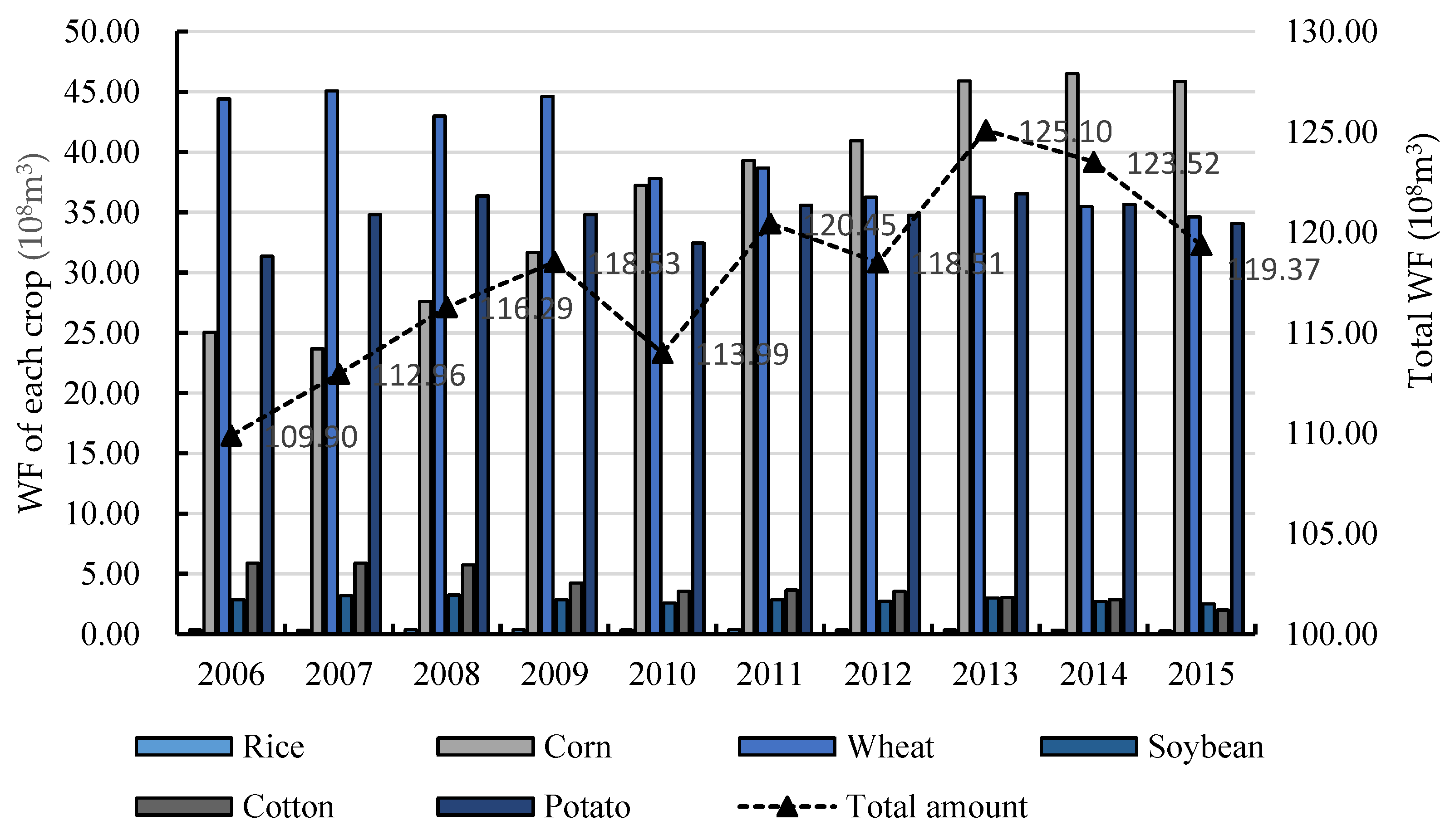
4.1.1. WF of Agriculture in Gansu Province
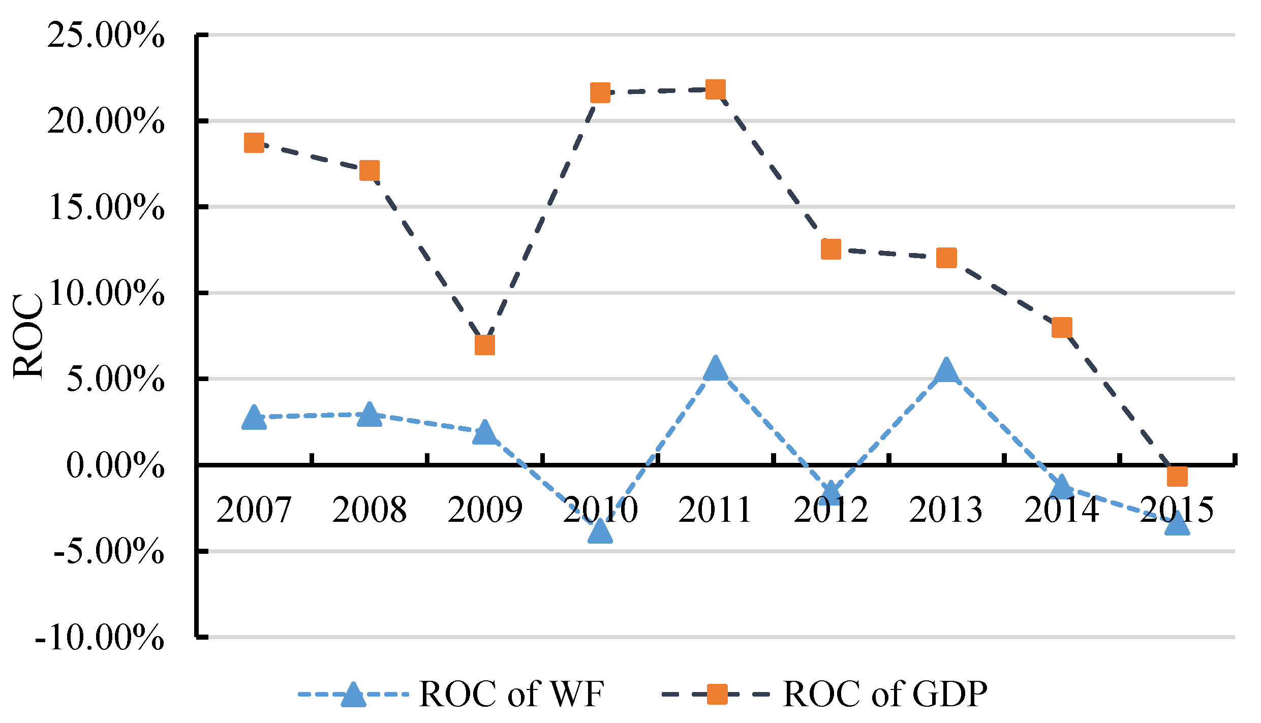
4.1.2. Relationship between Agricultural Economic Growth and WF Changes
4.2. Analysis of Driving Effects of Agricultural WF Changes
4.3. The Decoupling Relationship between Agricultural WF Changes and Agricultural Economic Growth
4.3.1. The Decoupling Status of Changes in Agricultural WF and Economic Growth
4.3.2. Analysis of Changes in Decoupling Factors of Agricultural WF
5. Conclusions
Author Contributions
Funding
Conflicts of Interest
References
- Dijkgraaf, E.; Vollebergh, H.R.J. A test for parameter homogeneity in CO2 panel EKC estimations. Environ. Resour. Econ. 2005, 32, 229–239. [Google Scholar] [CrossRef]
- Chen, L.; Chen, S. The estimation of environmental kuznets curve in China: Nonparametric panel approach. Comput. Econ. 2015, 46, 405–420. [Google Scholar] [CrossRef]
- Grossman, G.; Krueger, A. Economic growth and the environment. Q. J. Econ. 1995, 110, 353–377. [Google Scholar] [CrossRef] [Green Version]
- OECD. Indicators to Measure Decoupling of Environmental Pressure from Economic Growth; OECD: Paris, France, 2002. [Google Scholar]
- Allan, J.A. Fortunately there are substitutes for water otherwise our hydro-political futures would be impossible. In Priorities for Water Resources Allocation and Management; ODA: London, UK, 1993; pp. 13–26. [Google Scholar]
- Hoekstra, A.Y.; Hung, P.Q. Virtual Water Trade: A Quantification of Virtual Water Flows between Nations in Relation to International Crop Trade; Value of Water Research Report Series 11; UNESCO-IHE: Delft, The Netherlands, 2002. [Google Scholar] [CrossRef]
- Qiu, L.; Huang, J.Y.; Niu, W.J. Decoupling and driving factors of economic growth and groundwater consumption in the coastal areas of the yellow sea and the bohai sea. Sustainability 2018, 10, 4158. [Google Scholar] [CrossRef] [Green Version]
- Wang, Q.; Jiang, R.; Li, R.R. Decoupling analysis of economic growth from water use in City: A case study of Beijing, Shanghai, and Guangzhou of China. Sustain. Cities Soc. 2018, 41, 86–94. [Google Scholar] [CrossRef]
- Cai, H.; Mei, Y.D.; Chen, Y.Y. An analysis of a water use decoupling index and its spatial migration characteristics based on extracting trend components: A case study of the poyang lake basin. Water 2019, 11, 1027. [Google Scholar] [CrossRef] [Green Version]
- Zhao, H.; Lu, X.D.; Shao, Z.Z. Empirical analysis on relationship between water footprint of China’s textile industry and eco-environment. Ekoloji 2019, 28, 1067–1076. [Google Scholar]
- Tian, Y.H.; Ruth, M.; Zhu, D.J. Using the IPAT identity and decoupling analysis to estimate water footprint variations for five major food crops in China from 1978 to 2010. Sustainability 2017, 19, 2355–2375. [Google Scholar] [CrossRef]
- Zhang, Y.; Yang, Q.S. Decoupling agricultural water consumption and environmental impact from crop production based on the water footprint method: A case study for the Heilongjiang land reclamation area, China. Ecol. Indic. 2014, 43, 29–35. [Google Scholar] [CrossRef]
- Chapagain, A.K.; Hoekstra, A.Y. The blue, green and grey water footprint of rice from production and consumption perspectives. Ecol. Econ. 2011, 70, 749–758. [Google Scholar] [CrossRef]
- Chen, W.M.; Wu, S.M.; Lei, Y.L.; Li, S.T. China’s water footprint by province, and inter-provincial transfer of virtual water. Ecol. Indic. 2017, 74, 321–333. [Google Scholar] [CrossRef]
- Stella, S.; Dimitra, V. Water footprint of crops on rhodes island. Water 2019, 11, 1084. [Google Scholar] [CrossRef] [Green Version]
- Vale, R.L.; Netto, A.M.; de Lima Xavier, B.T.; de Lavor Paes Barreto, M.; da Silva, J.P.S. Assessment of the gray water footprint of the pesticide mixture in a soil cultivated with sugarcane in the northern area of the State of Pernambuco, Brazil. J. Clean. Prod. 2019, 234, 925–932. [Google Scholar] [CrossRef]
- Nezamoleslami, R.; Hosseinian, S.M. An improved water footprint model of steel production concerning virtual water of personnel: The case of Iran. J. Environ. Manag. 2020, 260, 110065. [Google Scholar] [CrossRef] [PubMed]
- Zheng, J.Z.; Wang, W.G.; Ding, Y.M.; Liu, G.S.; Xing, W.Q.; Cao, X.C.; Chen, D. Assessment of climate change impact on the water footprint in rice production: Historical simulation and future projections at two representative rice cropping sites of China. Sci. Total Environ. 2020, 709, 136190. [Google Scholar] [CrossRef] [PubMed]
- Ang, B.W.; Zhang, F.Q.; Choi, K.H. Factorizing changes in energy and environmental indicators through decomposition. Energy 1998, 23, 489–495. [Google Scholar] [CrossRef]
- Wu, Y.; Tam, V.W.Y.; Shuai, C.Y.; Shen, L.Y.; Zhang, Y.; Liao, S.J. Decoupling China’s economic growth from carbon emissions: Empirical studies from 30 Chinese provinces (2001–2015). Sci. Total Environ. 2019, 656, 576–588. [Google Scholar] [CrossRef] [PubMed]
- Zhao, R.Q.; Liu, Y.; Tian, M.M.; Ding, M.L.; Cao, L.H.; Zhang, Z.P.; Chuai, X.W.; Xiao, L.G.; Yao, L.G. Impacts of water and land resources exploitation on agricultural carbon emissions: The water-land-energy-carbon nexus. Land Use Policy 2018, 72, 480–492. [Google Scholar] [CrossRef]
- Yao, L.Q.; Xu, J.R.; Zhang, L.N.; Pang, Q.H.; Zhang, C.J. Temporal-spatial decomposition computing of regional water intensity for Yangtze River Economic Zone in China based on LMDI model. Sustain. Comput.-Inform. Syst. 2019, 21, 119–128. [Google Scholar] [CrossRef]
- Zhang, S.L.; Su, X.L.; Singh, V.P.; Olaitan, A.O.; Xie, J. Logarithmic Mean Divisia Index (LMDI) decomposition analysis of changes in agricultural water use: A case study of the middle reaches of the Heihe River basin, China. Agric. Water Manag. 2018, 208, 422–430. [Google Scholar] [CrossRef]
- Zou, M.Z.; Kang, S.Z.; Niu, J.; Lu, H.N. A new technique to estimate regional irrigation water demand and driving factor effects using an improved SWAT model with LMDI factor decomposition in an arid basin. J. Clean. Prod. 2018, 185, 814–828. [Google Scholar] [CrossRef]
- Zhao, C.F.; Chen, B. Driving force analysis of the agricultural water footprint in China based on the LMDI method. Environ. Sci. Technol. 2014, 48, 12723–12731. [Google Scholar] [CrossRef] [PubMed]
- Xu, Y.J.; Huang, K.; Yu, Y.J.; Wang, X.M. Changes in water footprint of crop production in Beijing from 1978 to 2012: A logarithmic mean Divisia index decomposition analysis. J. Clean. Prod. 2015, 87, 180–187. [Google Scholar] [CrossRef]
- Zhao, X.; Tillotson, M.R.; Liu, Y.W.; Guo, W.; Yang, A.H.; Li, Y.F. Index decomposition analysis of urban crop water footprint. Ecol. Model. 2017, 348, 25–32. [Google Scholar] [CrossRef] [Green Version]
- Liang, W.; Gan, T.; Zhang, W. Dynamic evolution of characteristics and decomposition of factors influencing industrial carbon dioxide emissions in China: 1991-2015. Struct. Chang Econ. Dyn. 2019, 49, 93–106. [Google Scholar] [CrossRef]
- Wang, S.S.; Li, R.R. Toward the coordinated sustainable development of urban water resource use and economic growth: An empirical analysis of Tianjin City, China. Sustainability 2018, 10, 1323. [Google Scholar] [CrossRef] [Green Version]
- Li, Y.; Lu, L.Y.; Tan, Y.X.; Wang, L.L. Decoupling water consumption and environmental impact on textile industry by using water footprint method: A case study in China. Water 2017, 9, 124. [Google Scholar] [CrossRef]
- Hoekstra, A.Y.; Chapagain, A.K.; Aldaya, M.M.; Mekonnen, M.M. Water Footprint Manual: State of the Art 2009; Water Footprint Network: Enschede, The Netherlands, 2009. [Google Scholar]
- Gu, Y.F.; Xu, J.; Wang, H.T.; Li, F.T. Industrial water footprint assessment: Methodologies in need of improvement. Environ. Sci. Technol. 2014, 5, 6531–6532. [Google Scholar] [CrossRef]
- Egan, M. The Water Footprint Assessment Manual. Setting the Global Standard. Soc. Environ. Account. J. 2011, 31, 181–182. [Google Scholar] [CrossRef]
- Chapagain, A.K.; Orr, S. An improved water footprint methodology linking global consumption to local water resources: A case of Spanish tomatoes. J. Environ. Manage. 2008, 90, 1219–1228. [Google Scholar] [CrossRef]
- Aldaya, M.M.; Llamas, M.R. Water Footprint Analysis for the Guadiana River Basin; Value of Water Research Report Series No. 35; UNESCO-IHE: Delft, The Netherlands, 2008; Available online: https://www.waterfootprint.org/Reports/Report35-WaterFootprint-Guadiana.pdf (accessed on 28 July 2020).
- Oel, V.P.R.; Mekonnen, M.M.; Hoekstra, A.Y. The external water footprint of the Netherlands: Quantification and impact assessment. Ecol. Econ. 2008, 69, 82–92. [Google Scholar]
- Chapagain, A.K.; Hoekstra, A.Y.; Savenije, H.H.G.; Gautam, R. The water footprint of cotton consumption: An assessment of the impact of worldwide consumption of cotton products on the water resources in the cotton producing countries. Ecol. Econ. 2006, 60, 186–203. [Google Scholar] [CrossRef]
- Allen, R.G.; Pereira, L.S.; Raes, D.; Smith, M. Crop Evapotranspiration-Guidelines for Computing Crop Water Requirements-FAO Irrigation and Drainage; Food and Agriculture Organization: Rome, Italy, 1998; p. 56. [Google Scholar]
- Hatzigeorgiou, E.; Polatidis, H.; Haralambopoulos, D. CO2 emissions in Greece for 1990–2002: A decomposition analysis and comparison of results using the Arithmetic Mean Divisia Index and Logarithmic Mean Divisia Index techniques. Energy 2008, 33, 492–499. [Google Scholar] [CrossRef]
- Wang, C.; Chen, J.N.; Zou, J. Decomposition of energy-related CO2 emission in China: 1957–2000. Energy 2005, 30, 73–83. [Google Scholar] [CrossRef]
- Ang, B.W. Decomposition analysis for policymaking in energy: Which is the preferred method? Energy Policy 2004, 32, 1131–1139. [Google Scholar] [CrossRef]
- Zhang, Y.F.; Yang, D.G.; Tang, H.; Liu, Y.X. Analyses of the changing process and influencing factors of water resource utilization in megalopolis of arid area. Water Resour. 2015, 42, 712–720. [Google Scholar] [CrossRef]
- Shang, Y.Z.; Lu, S.B.; Shang, L.; Li, X.F.; Wei, Y.P.; Lei, X.H.; Wang, C.; Wang, H. Decomposition methods for analyzing changes of industrial water use. J. Hydrol. 2016, 543, 808–817. [Google Scholar] [CrossRef] [Green Version]
- Zhang, L.; Dong, H.J.; Geng, Y.; Francisco, M.J. China’s provincial grey water footprint characteristic and driving forces. Sci. Total Environ. 2019, 677, 427–435. [Google Scholar] [CrossRef]
- Kang, J.F.; Lin, J.Y.; Zhao, X.F.; Zhao, S.N.; Kou, L.M. Decomposition of the urban water footprint of food consumption: A case study of Xiamen City. Sustainability 2017, 9, 135. [Google Scholar] [CrossRef] [Green Version]
- Yang, C.; Cui, X.F. Global changes and drivers of the water footprint of food consumption: A historical analysis. Water 2014, 6, 1435–1452. [Google Scholar] [CrossRef] [Green Version]


| Decoupling | ΔGDP | ΔWF | D(WF,GDP) | Status Description | |
|---|---|---|---|---|---|
| Type | Status | ||||
| Coupling | expansive | >0 | >0 | 0.8 ≤ D ≤ 1.2 | Both increase, relatively synchronized |
| recessive | <0 | <0 | 0.8 ≤ D ≤ 1.2 | Both decrease, relatively synchronized | |
| Decoupling | weak | >0 | >0 | 0 ≤ D < 0.8 | Both increase, GDP changes faster |
| strong | >0 | <0 | D < 0 | GDP increases, WF decreases, best status | |
| recessive | <0 | <0 | D > 1.2 | Both decrease, WF changes faster | |
| Negative decoupling | expansive | >0 | >0 | D > 1.2 | Both increase, WF changes faster |
| strong | <0 | >0 | D < 0 | WF increases, GDP decreases, worst status | |
| weak | <0 | <0 | 0 ≤ D < 0.8 | Both decrease, GDP changes faster | |
| Year | ΔWFI | ΔWFS | ΔWFC | ΔWFP | Total Effect | Principal Factor | |
|---|---|---|---|---|---|---|---|
| Stimulative | Withholder | ||||||
| 2006–2007 | −15.22 | 1.85 | 18.29 | −1.86 | 3.06 | economic * | technological |
| 2007–2008 | −12.82 | 5.42 | 12.8 | −2.08 | 3.33 | economic | technological * |
| 2008–2009 | −9.56 | 1.37 | 12.6 | −2.17 | 2.24 | economic * | technological |
| 2009–2010 | −33.15 | 13.16 | 17.51 | −2.04 | −4.53 | economic | technological * |
| 2010–2011 | −7.72 | 3.55 | 12.28 | −1.66 | 6.45 | economic * | technological |
| 2011–2012 | −20.28 | 4.53 | 16.29 | −2.47 | −1.93 | economic | technological * |
| 2012–2013 | −8.6 | 3.07 | 14.68 | −2.57 | 6.58 | economic * | technological |
| 2013–2014 | −10.21 | 2.39 | 9.09 | −2.85 | −1.58 | economic | technological * |
| 2014–2015 | −12.26 | 1.1 | 9.77 | −2.76 | −4.15 | economic | technological * |
| 2006–2015 | −643.24 | 51.74 | 782.76 | −77.99 | 113.27 | economic * | technological |
| 11th five-year | −78.48 | 25.35 | 73.48 | −9.8 | 10.55 | economic | technological * |
| 12th five-year | −59.07 | 14.64 | 62.12 | −12.31 | 5.37 | economic * | technological |
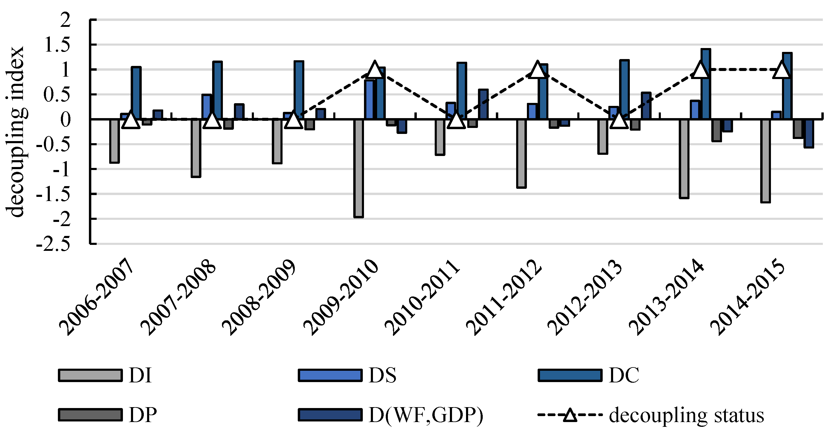
| Year | DI | DS | DC | DP | D(WF,GDP) | Status |
|---|---|---|---|---|---|---|
| 2006–2007 | −0.87 | 0.11 | 1.05 | −0.11 | 0.18 | weak |
| 2007–2008 | −1.16 | 0.49 | 1.16 | −0.19 | 0.30 | weak |
| 2008–2009 | −0.88 | 0.13 | 1.17 | −0.20 | 0.21 | weak |
| 2009–2010 | −1.97 | 0.78 | 1.04 | −0.12 | −0.27 | strong |
| 2010–2011 | −0.71 | 0.33 | 1.14 | −0.15 | 0.60 | weak |
| 2011–2012 | −1.37 | 0.31 | 1.10 | −0.17 | −0.13 | strong |
| 2012–2013 | −0.69 | 0.25 | 1.18 | −0.21 | 0.53 | weak |
| 2013–2014 | −1.58 | 0.37 | 1.41 | −0.44 | −0.24 | strong |
| 2014–2015 | −1.67 | 0.15 | 1.33 | −0.38 | −0.57 | strong |
© 2020 by the authors. Licensee MDPI, Basel, Switzerland. This article is an open access article distributed under the terms and conditions of the Creative Commons Attribution (CC BY) license (http://creativecommons.org/licenses/by/4.0/).
Share and Cite
Shi, C.; Yuan, H.; Pang, Q.; Zhang, Y. Research on the Decoupling of Water Resources Utilization and Agricultural Economic Development in Gansu Province from the Perspective of Water Footprint. Int. J. Environ. Res. Public Health 2020, 17, 5758. https://0-doi-org.brum.beds.ac.uk/10.3390/ijerph17165758
Shi C, Yuan H, Pang Q, Zhang Y. Research on the Decoupling of Water Resources Utilization and Agricultural Economic Development in Gansu Province from the Perspective of Water Footprint. International Journal of Environmental Research and Public Health. 2020; 17(16):5758. https://0-doi-org.brum.beds.ac.uk/10.3390/ijerph17165758
Chicago/Turabian StyleShi, Changfeng, Hang Yuan, Qinghua Pang, and Yangyang Zhang. 2020. "Research on the Decoupling of Water Resources Utilization and Agricultural Economic Development in Gansu Province from the Perspective of Water Footprint" International Journal of Environmental Research and Public Health 17, no. 16: 5758. https://0-doi-org.brum.beds.ac.uk/10.3390/ijerph17165758