Comparative Study of Hydrochemical Classification Based on Different Hierarchical Cluster Analysis Methods


Abstract
:1. Introduction
2. Materials and Methods
2.1. General Setting of the Study Area
2.2. Sample Collections
2.3. Chemical Analyses
2.4. Data Quality Assurance
2.5. Cluster Analysis (CA)
2.5.1. Concept
2.5.2. Hierarchical Cluster Analysis
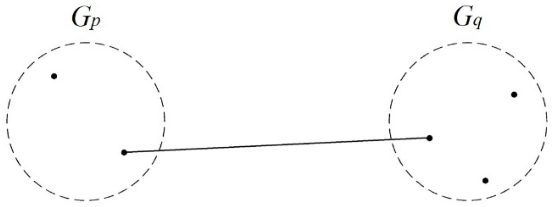
Single Linkage
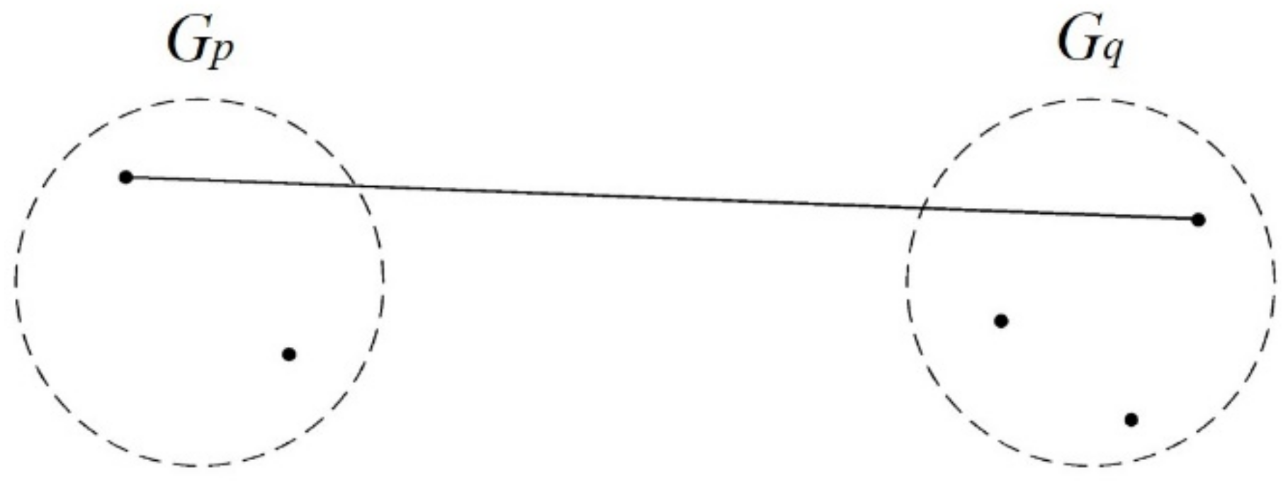
Complete Linkage
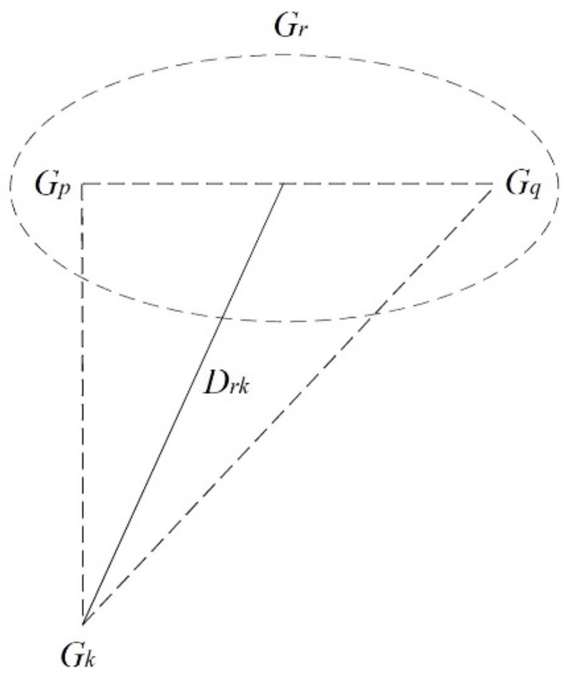
Median Linkage
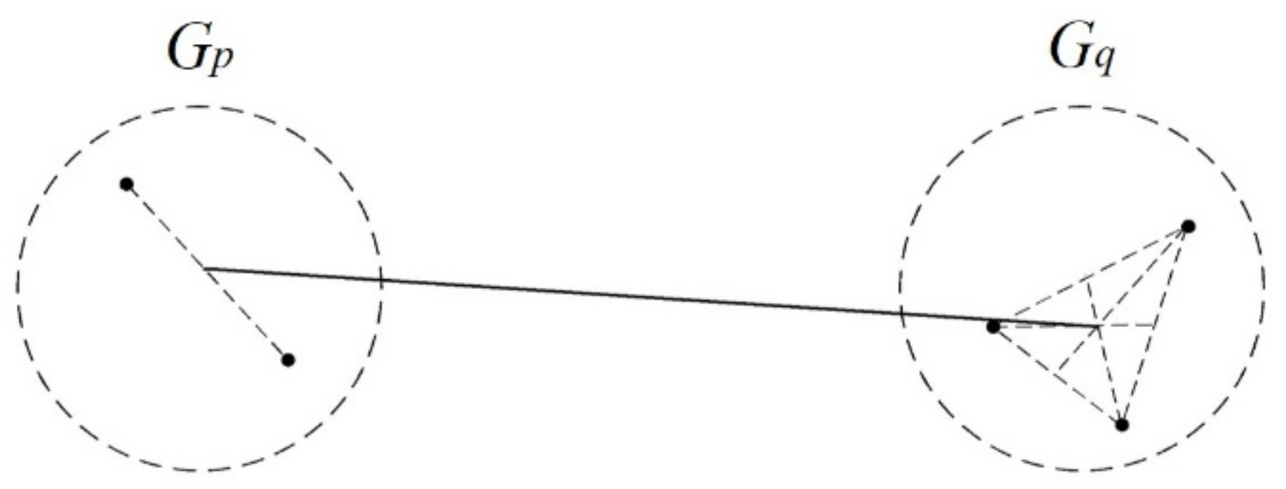
Centroid Linkage
Average Linkage
- a.
- Between-groups linkage
- b.
- Within-groups linkage
Ward’s Minimum-Variance
2.5.3. Data Standardization
2.5.4. Euclidean Distance
3. Results
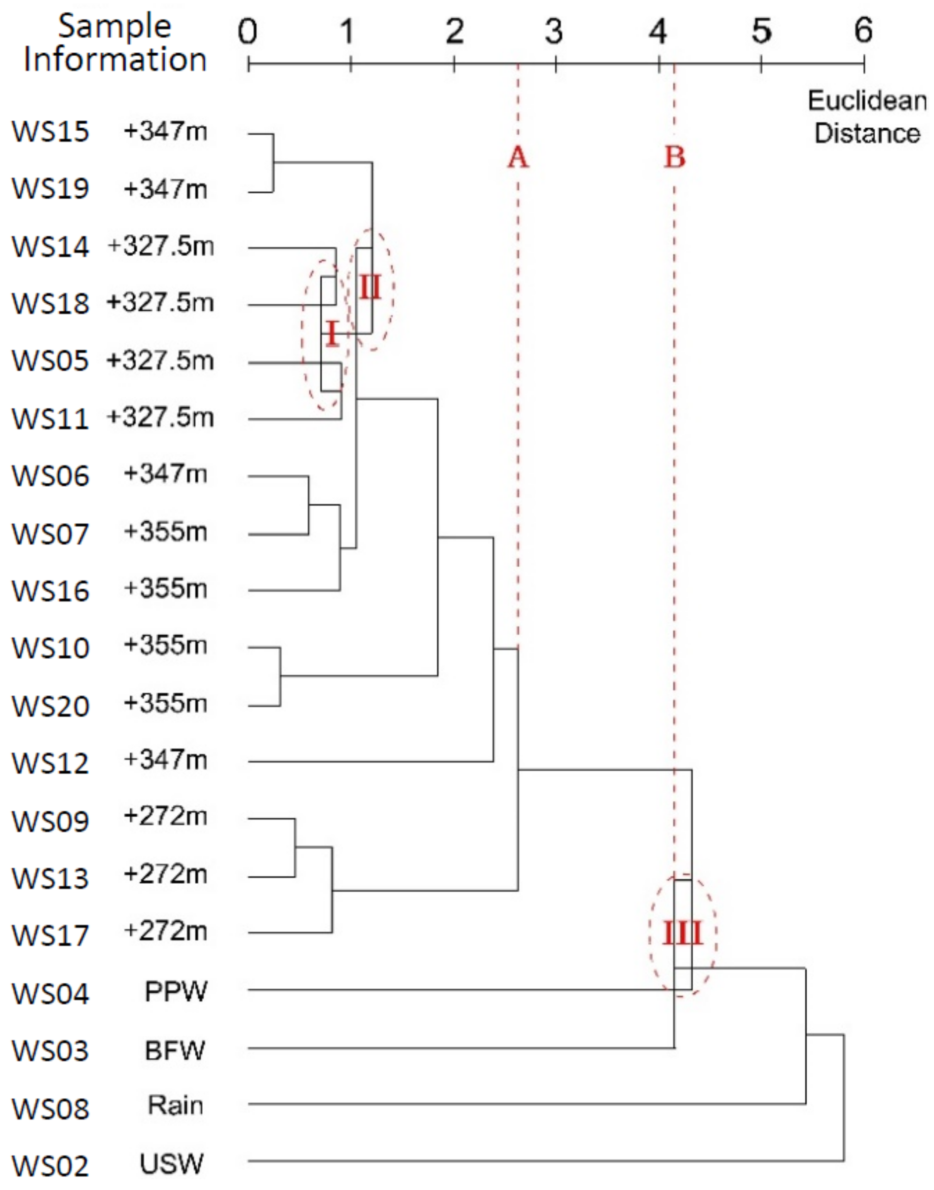
3.1. Single Linkage Method
3.2. Complete Linkage Method
3.3. Median Linkage Method
3.4. Centroid Linkage Method
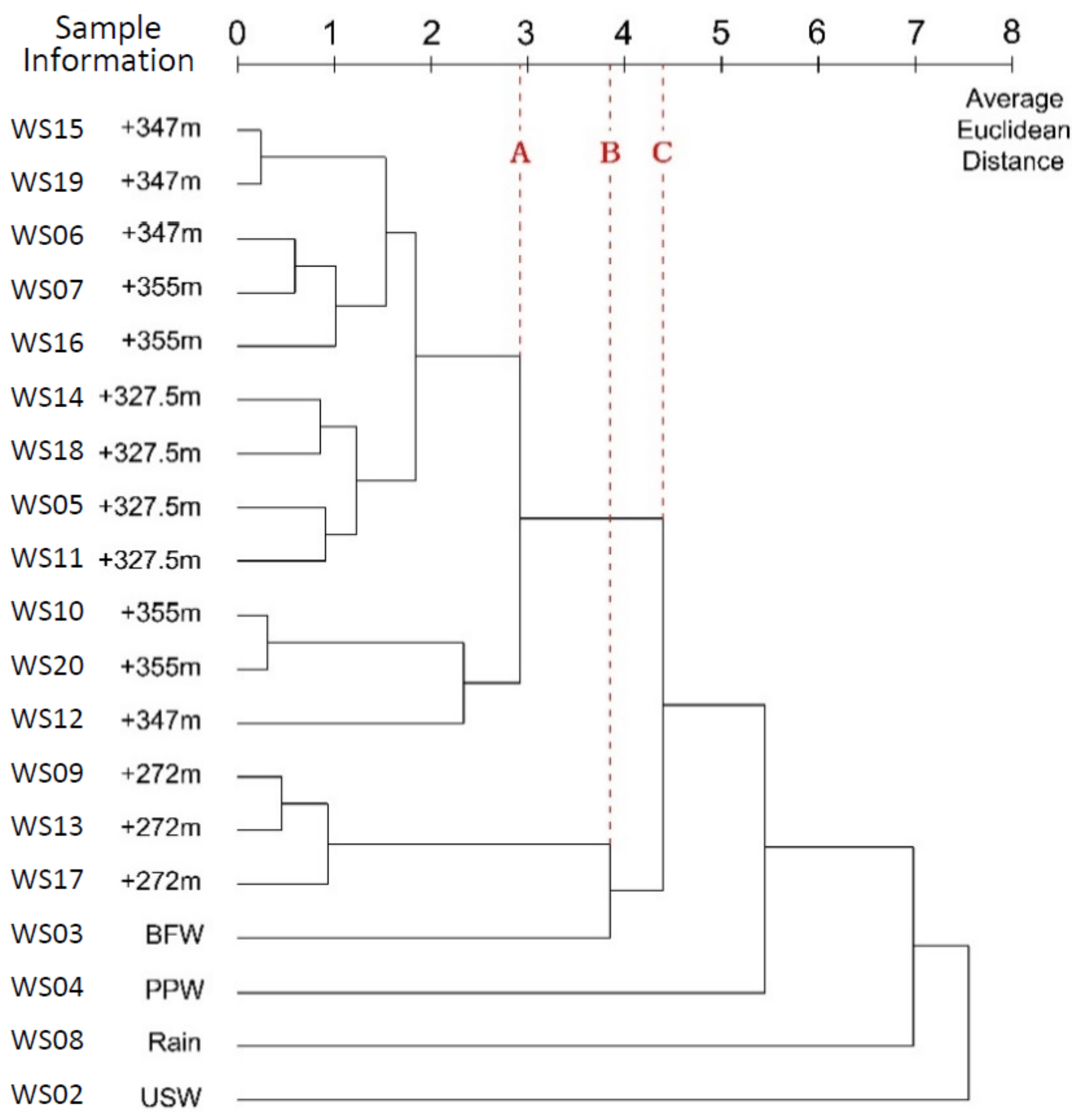
3.5. Average Linkage Method
3.5.1. Between-Groups Linkage
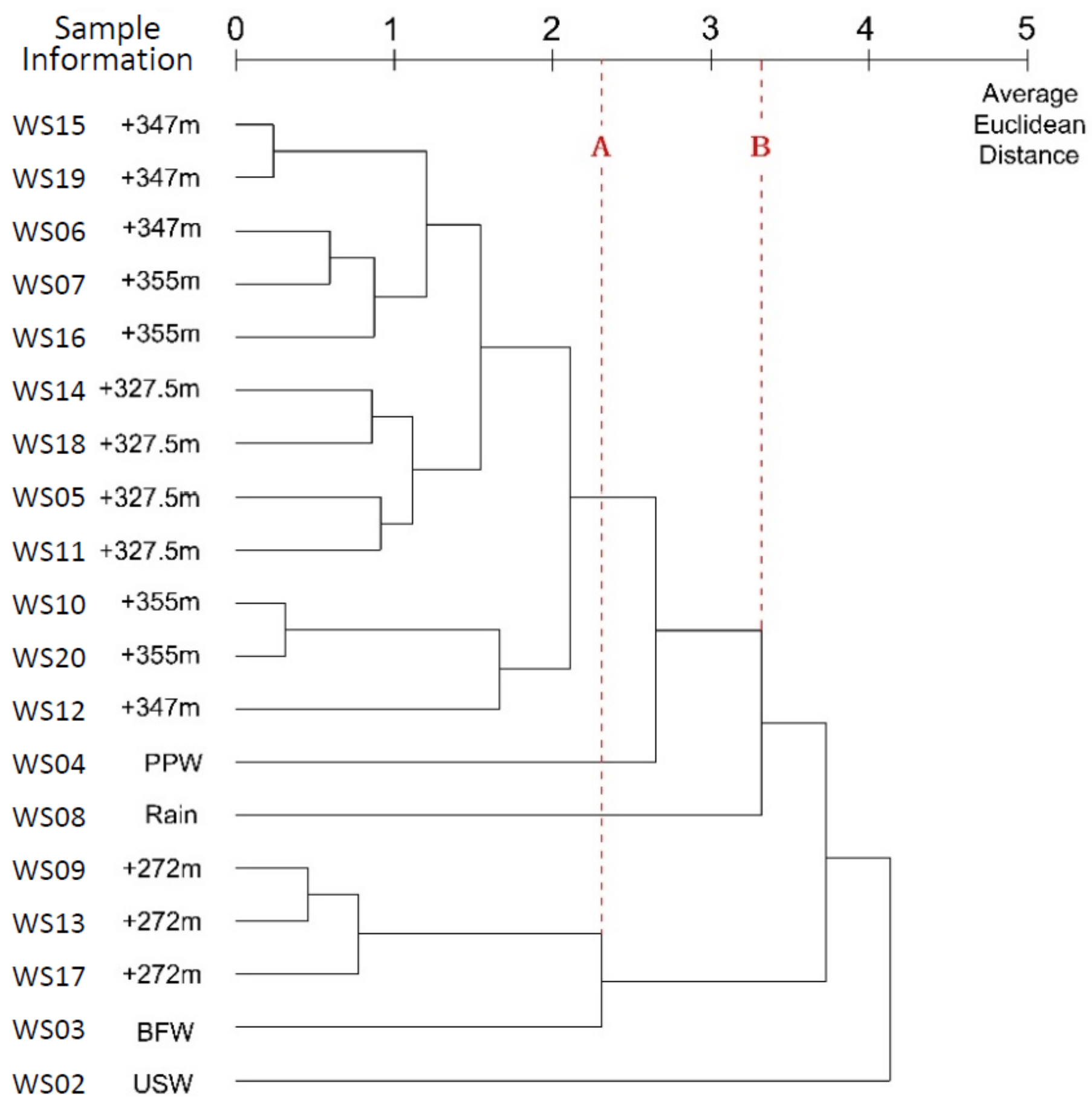
3.5.2. Within-Groups Linkage
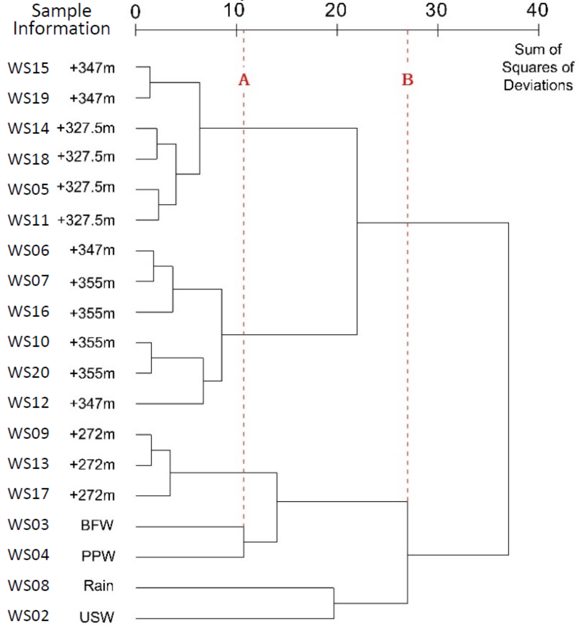
3.6. Ward’s Minimum-Variance Method
4. Discussion
4.1. Single Linkage Method
4.2. Complete Linkage Method
4.3. Median Linkage Method
4.4. Centroid Linkage Method
4.5. Average Linkage Method
4.5.1. Between-Groups Linkage
4.5.2. Within-Groups Linkage
4.6. Ward’s Minimum-Variance Method
4.7. Hydrochemical Characteristics
5. Conclusions
- (1)
- In the HCA, single linkage was the most basic, comprehensible, and accessible method, which reflected the concept of hierarchical clustering directly. However, it was limited by little differentiations in clustering steps and the inevitable linking tendency (as seen from the ladder-like shapes in dendrograms). Complete linkage adjusted and improved the basis of single linkage. It avoided the inevitable generation of links and ladder-shaped dendrograms. By increasing the distance between clusters for merging, clustering with complete linkage was more refined and data sensitive. However, both single and complete linkage were significantly affected by outliers, and were therefore ineffective when processing data with large dispersions;
- (2)
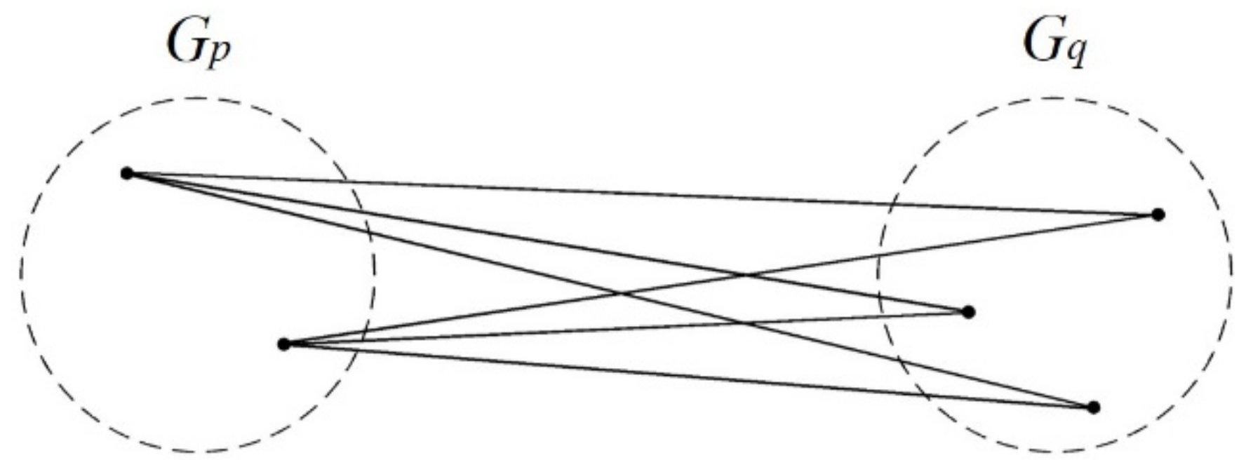
- Unlike single and complete linkage, median linkage avoided measuring extreme distances, whereas centroid linkage emphasized the representativeness of a cluster. The centroids of clusters had to be recalculated each time after every two clusters merged; therefore, centroid linkage performed more stably when dealing with outliers. However, given the non-monotonicity of these two methods, the distance for merging was likely less than the distance in the previous step, which may have led to reversals, partially closed and crossing links, or other issues in dendrograms. Therefore, these two methods were not recommended;
- (3)
- Average linkage was the default method in the HCA module in SPSS. It included two techniques (i.e., between-group linkage and within-group linkage), and both could make full use of known information. All samples and indicators were considered, and the clustering process was not easily affected by outliers. Average linkage performed well in clustering and was recommended for dealing with a large number of samples, complex variables, and indicators;
- (4)
- Ward’s minimum-variance method could capture and enlarge the differences between clusters that were subtle, hidden, and difficult to identify using other methods, which was conducive to data classification. Using this method, more information could be delivered and expressed, which increased the classification accuracy. For classification tasks with fewer objects and variables, this method could effectively improve the accuracy and classification sensitivity, which could help to explore the essential attributes of data.
Author Contributions
Funding
Conflicts of Interest
References
- Liang, Y.; Ma, R.; Wang, Y.; Wang, S.; Qu, L.; Wei, W.; Gan, Y. Hydrogeological controls on ammonium enrichment in shallow groundwater in the central Yangtze River Basin. Sci. Total Environ. 2020, 741, 140350. [Google Scholar] [CrossRef]
- Hu, Y.; Ma, R.; Wang, Y.; Chang, Q.; Wang, S.; Ge, M.; Bu, J.; Sun, Z. Using hydrogeochemical data to trace groundwater flow paths in a cold alpine catchment. Hydrol. Process. 2019, 33, 1942–1960. [Google Scholar] [CrossRef]
- Chang, Q.; Ma, R.; Sun, Z.; Zhou, A.; Hu, Y.; Liu, Y. Using isotopic and geochemical tracers to determine the contribution of glacier-snow meltwater to streamflow in a partly glacierized alpine-gorge catchment in northeastern Qinghai-Tibet Plateau. J. Geophys. Res. Atmos. 2018, 123, 10037–10056. [Google Scholar] [CrossRef]
- Ma, R.; Sun, Z.; Hu, Y.; Chang, Q.; Wang, S.; Xing, W.; Ge, M. Hydrological connectivity from glaciers to rivers in the Qinghai–Tibet Plateau: Roles of suprapermafrost and subpermafrost groundwater. Hydrol. Earth Syst. Sci. 2017, 21, 4803–4823. [Google Scholar] [CrossRef] [Green Version]
- Lin, J.; Ma, R.; Hu, Y.; Sun, Z.; Wang, Y.; McCarter, C.P. Groundwater sustainability and groundwater/surface-water interaction in arid Dunhuang Basin, northwest China. Hydrogeol. J. 2018, 26, 1559–1572. [Google Scholar] [CrossRef]
- Guler, C.; Thyne, G.D. Hydrologic and geologic factors controlling surface and groundwater chemistry in Indian Wells-Owens Valley area, southeastern California, USA. J. Hydrol. 2004, 285, 177–198. [Google Scholar] [CrossRef]
- Bu, J.; Sun, Z.; Ma, R.; Liu, Y.; Gong, X.; Pan, Z.; Wei, W. Shallow Groundwater Quality and Its Controlling Factors in the Su-Xi-Chang Region, Eastern China. Int. J. Environ. Res. Public Health 2020, 17, 1267. [Google Scholar] [CrossRef] [PubMed] [Green Version]
- Zhang, B.; Song, X.; Zhang, Y.; Han, D.; Tang, C.; Yu, Y.; Ma, Y. Hydrochemical characteristics and water quality assessment of surface water and groundwater in Songnen plain, Northeast China. Water Res. 2012, 46, 2737–2748. [Google Scholar] [CrossRef]
- Zhang, Q.; Wang, S.; Yousaf, M.; Wang, S.; Nan, Z.; Ma, J.; Wang, D.; Zang, F. Hydrochemical characteristics and water quality assessment of surface water in the northeast Tibetan Plateau of China. Water Sci. Technol. 2018, 18, 1757–1768. [Google Scholar] [CrossRef]
- Gu, H.; Chi, B.; Li, H.; Jiang, J.; Qin, W.; Wang, H. Assessment of groundwater quality and identification of contaminant sources of Liujiang basin in Qinhuangdao, North China. Environ. Earth Sci. 2015, 73, 6477–6493. [Google Scholar] [CrossRef]
- Zhang, Q.; Wang, S.; Yousaf, M.; Nan, Z.; Wang, S.; Ma, J.; Wang, D.; Zang, F. Hydrochemical Characteristics and Water Quality Assessment of Surface Water at Xiahe County in Tibetan Plateau Pastoral of China. Preprints 2016. [Google Scholar] [CrossRef]
- Miranda, J.; Andrade, E.; López-Suárez, A.; Ledesma, R.; Cahill, T.A.; Wakabayashi, P.H. A receptor model for atmospheric aerosols from a southwestern site in Mexico city. Atmos. Environ. 1996, 30, 3471–3479. [Google Scholar] [CrossRef]
- Vega, M.; Pardo, R.; Barrado, E.; Debán, L. Assessment of seasonal and polluting effects on the quality of river water by exploratory data analysis. Water Res. 1998, 32, 3581–3592. [Google Scholar] [CrossRef]
- Chen, K.; Jiao, J.J.; Huang, J.; Huang, R. Multivariate statistical evaluation of trace elements in groundwater in a coastal area in Shenzhen, China. Environ. Pollut. 2007, 147, 771–780. [Google Scholar] [CrossRef] [PubMed]
- Güler, C.; Thyne, G.D.; McCray, J.E.; Turner, K.A. Evaluation of graphical and multivariate statistical methods for classification of water chemistry data. Hydrogeol. J. 2002, 10, 455–474. [Google Scholar] [CrossRef]
- Goné, D.L.; Douagui, A.G.; Bai, L.; Kamagaté, B.; Ligban, R. Using Graphical and Multivariate Statistical Methods for Geochemical Assessment of Groundwater Quality in Oumé Department (Cte d’Ivoire). J. Environ. Prot. 2014, 5, 1265. [Google Scholar]
- Aruga, R.; Negro, G.; Ostacoli, G. Multivariate data analysis applied to the investigation of river pollution. Fresenius J. Anal. Chem. 1993, 346, 968–975. [Google Scholar] [CrossRef]
- Ritzi, R.W., Jr.; Wright, S.L.; Mann, B.; Chen, M. Analysis of Temporal Variability in Hydrogeochemical Data Used for Multivariate Analyses. Groundwater 2010, 31, 221–229. [Google Scholar] [CrossRef]
- Usunoff, E.J.; Guzmán-Guzmán, A. Multivariate Analysis in Hydrochemistry: An Example of the Use of Factor and Correspondence Analyses. Groundwater 1989, 27, 27–34. [Google Scholar] [CrossRef]
- Ashley, R.P.; Lloyd, J.W. An example of the use of factor analysis and cluster analysis in groundwater chemistry interpretation. J. Hydrol. 1978, 39, 355–364. [Google Scholar] [CrossRef]
- Panda, U.C.; Sundaray, S.K.; Rath, P.; Nayak, B.B.; Bhatta, D. Application of factor and cluster analysis for characterization of river and estuarine water systems-A case study: Mahanadi River (India). J. Hydrol. 2006, 331, 434–455. [Google Scholar] [CrossRef]
- Swanson, S.K.; Bahr, J.M.; Schwar, M.T. Two-way Cluster Analysis of Geochemical Data to Constrain Spring Source Waters. Chem. Geol. 2001, 179, 73–91. [Google Scholar] [CrossRef]
- Walton, N.R.G. Electrical Conductivity and Total Dissolved Solids—What is Their Precise Relationship? Desalination 1989, 72, 275–292. [Google Scholar] [CrossRef]
- Atekwana, E.A.; Atekwana, E.A.; Rowe, R.S.; Werkema, D.D., Jr.; Legall, F.D. The relationship of total dissolved solids measurements to bulk electrical conductivity in an aquifer contaminated with hydrocarbon. J. Appl. Geophys. 2004, 56, 281–294. [Google Scholar] [CrossRef]
- Marickar, Y.M.F. Electrical conductivity and total dissolved solids in urine. Urol. Res. 2010, 38, 233–235. [Google Scholar] [CrossRef] [PubMed]
- APHA/AWWA/WEF. Standard Methods for the Examination of Water and Wastewater, 21st ed.; American Public Health Association: Washington, DC, USA, 2005. [Google Scholar]
- Bu, J.; Sun, Z.; Zhou, A.; Xu, Y.; Ma, R.; Wei, W.; Liu, M. Heavy metals in surface soils in the upper reaches of the Heihe River, northeastern Tibetan Plateau, China. Int. J. Environ. Res. Public Health 2016, 13, 247. [Google Scholar] [CrossRef] [Green Version]
- DíAz, R.V.; Aldape, F.; Flores, M.J. Identification of airborne particulate sources, of samples collected in Ticomán, Mexico, using pixe and multivariate analysis. Nucl. Instrum. Methods Phys. Res. 2002, 189, 249–253. [Google Scholar] [CrossRef]
- Han, Y.M.; Du, P.X.; Cao, J.J.; Posmentier, E.S. Multivariate analysis of heavy metal contamination in urban dusts of Xi’an, central China. Sci. Total Environ. 2006, 355, 176–186. [Google Scholar]
- Bu, J.W.; Zhou, J.W.; Zhou, A.G.; Kong, F.L. The Comparison of Different Methods in Hydrochemical Classification Using Hierarchical Clustering Analysis. In Proceedings of the 2011 International Conference on Remote Sensing, Environment and Transportation Engineering (RSETE), Nanjing, China, 24–26 June 2011; IEEE: Piscataway, NJ, USA, 2011; pp. 1783–1787. [Google Scholar]
- Suk, H.; Lee, K.K. Characterization of a Ground Water Hydrochemical System Through Multivariate Analysis: Clustering. Ground Water 1999, 37, 358. [Google Scholar] [CrossRef]
- Rafighdoust, Y.; Eckstein, Y.; Harami, R.M.; Gharaie, M.H.M.; Mahboubi, A. Using inverse modeling and hierarchical cluster analysis for hydrochemical characterization of springs and Talkhab River in Tang-Bijar oilfield, Iran. Arab. J. Geosci. 2016, 9, 241. [Google Scholar] [CrossRef]
- Tay, C.K.; Hayford, E.; Hodgson, I.O.; Kortatsi, B.K. Hydrochemical appraisal of groundwater evolution within the Lower Pra Basin, Ghana: A hierarchical cluster analysis (HCA) approach. Environ. Earth Sci. 2015, 73, 3579–3591. [Google Scholar] [CrossRef]
- Gorman, B.S.; Primavera, L.H. The Complementary Use of Cluster and Factor Analysis Methods. J. Exp. Educ. 1983, 51, 165–168. [Google Scholar] [CrossRef]
- Li, G.; Wang, X.; Meng, Z.; Zhao, H. Seawater inrush assessment based on hydrochemical analysis enhanced by hierarchy clustering in an undersea goldmine pit, China. Environ. Earth Sci. 2014, 71, 4977–4987. [Google Scholar] [CrossRef]
- Helstrup, T.; Jrgensen, N.O.; Banoeng-Yakubo, B. Investigation of hydrochemical characteristics of groundwater from the Cretaceous-Eocene limestone aquifer in southern Ghana and southern Togo using hierarchical cluster analysis. Hydrogeol. J. 2007, 15, 977–989. [Google Scholar] [CrossRef]


| Sample Number | Sampling Location | Water Type | pH | Na+ | K+ | Ca2+ | Mg2+ | Cl− | SO42− | CO32− | HCO3− | F− | NO3− | TDS |
|---|---|---|---|---|---|---|---|---|---|---|---|---|---|---|
| WS 02 | CEMC | USW | 7.03 | 123.396 | 16.348 | 58.096 | 14.251 | 231.87 | 68.41 | - | 357.60 | 0.31 | - | 897.484 |
| WS 03 | Jianxinpo tunnel | BFW | 9.27 | 93.060 | 14.991 | 103.398 | 0.926 | 24.35 | 81.95 | 83.52 | 9.57 | 1.39 | 67.92 | 523.827 |
| WS 04 | Jianxinpo tunnel | PPW | 9.62 | 77.533 | 13.630 | 233.702 | 3.771 | 26.33 | 117.23 | 153.52 | 29.30 | 0.74 | 6.03 | 728.329 |
| WS 05 | +327.5 m | LW | 9.43 | 225.495 | 128.598 | 6.641 | 0.185 | 43.92 | 158.71 | 271.16 | 13.16 | 1.12 | 4.48 | 925.866 |
| WS 06 | +347 m | LW | 8.64 | 242.497 | 104.697 | 2.948 | 0.252 | 45.85 | 190.27 | 142.34 | 220.06 | 1.10 | 3.64 | 1038.044 |
| WS 07 | +355 m | LW | 8.69 | 233.404 | 103.904 | - | - | 44.98 | 220.18 | 145.28 | 211.09 | 1.11 | 0.94 | 1042.903 |
| WS 08 | Tunnel periphery | Rain | 5.37 | 6.161 | 2.555 | 0.908 | - | 4.46 | 10.77 | - | 34.68 | 0.08 | 7.88 | 71.649 |
| WS 09 | +272 m | DHRW | 8.72 | 111.902 | 11.661 | 0.848 | 0.103 | 44.74 | 82.59 | 65.29 | 81.33 | 1.28 | 11.60 | 445.418 |
| WS 10 | +355 m | LW | 8.58 | 261.199 | 134.796 | 10.964 | 0.941 | 47.43 | 197.10 | 94.11 | 400.66 | 1.04 | 5.47 | 1234.969 |
| WS 11 | +327.5 m | LW | 8.82 | 213.104 | 119.203 | 2.292 | 1.194 | 42.98 | 154.31 | 249.98 | 43.65 | 1.20 | 10.63 | 906.029 |
| WS 12 | +347 m | LW | 8.66 | 233.002 | 98.785 | 3.634 | 0.795 | 58.67 | 195.06 | 83.52 | 429.36 | 0.24 | 9.80 | 1178.830 |
| WS 13 | +272 m | DHRW | 8.84 | 120.696 | 14.640 | 0.303 | 0.171 | 43.67 | 82.79 | 88.23 | 41.26 | 1.35 | 15.43 | 445.471 |
| WS 14 | +327.5 m | LW | 9.48 | 212.302 | 110.803 | - | - | 41.35 | 139.92 | 131.76 | 13.16 | 1.21 | 2.77 | 718.916 |
| WS 15 | +347 m | LW | 8.41 | 218.403 | 82.868 | 1.517 | 0.084 | 46.87 | 148.38 | 54.11 | 134.55 | 1.12 | 2.47 | 759.789 |
| WS 16 | +355 m | LW | 8.51 | 239.996 | 118.797 | 3.695 | 2.016 | 42.06 | 170.79 | 200.57 | 188.97 | 1.02 | 5.73 | 1042.38 |
| WS 17 | +272 m | DHRW | 8.73 | 134.504 | 15.554 | 2.054 | 0.230 | 43.62 | 84.86 | 68.23 | 56.21 | 1.29 | 26.87 | 470.354 |
| WS 18 | +327.5 m | LW | 9.14 | 217.597 | 98.575 | 0.305 | 0.483 | 40.60 | 111.51 | 123.52 | 17.94 | 1.03 | 2.39 | 670.903 |
| WS 19 | +347 m | LW | 8.38 | 230.903 | 84.268 | 0.728 | 0.046 | 45.88 | 145.72 | 52.94 | 146.51 | 1.08 | 2.22 | 779.646 |
| WS 20 | +355 m | LW | 8.53 | 258.095 | 125.765 | 4.475 | 0.411 | 44.26 | 197.35 | 108.82 | 397.67 | 1.06 | 3.96 | 1221.649 |
| Sample Number | pH | Na+ | K+ | Ca2+ | Mg2+ | Cl− | SO42− | HCO3− | F− | NO3− | TDS |
|---|---|---|---|---|---|---|---|---|---|---|---|
| WS 02 | −1.61573 | −0.79248 | −1.15515 | 0.61412 | 3.96129 | 3.99725 | −1.19004 | 1.41 | −1.80109 | −0.65175 | 0.33212 |
| WS 03 | 0.73282 | −1.20678 | −1.18254 | 1.40611 | −0.13248 | −0.58216 | −0.9467 | −0.93993 | 1.06835 | 3.76961 | −0.87724 |
| WS 04 | 1.09978 | −1.41884 | −1.20993 | 3.68417 | 0.74037 | −0.53847 | −0.31265 | −0.80671 | −0.65863 | −0.25922 | −0.21535 |
| WS 05 | 0.90057 | 0.60173 | 1.10549 | −0.28557 | −0.35991 | −0.1503 | 0.43283 | −0.91569 | 0.35099 | −0.36012 | 0.42401 |
| WS 06 | 0.07229 | 0.83387 | 0.62416 | −0.35008 | −0.34147 | −0.10771 | 1.00003 | 0.48132 | 0.29785 | −0.4148 | 0.78706 |
| WS 07 | 0.12471 | 0.70961 | 0.60805 | −0.40166 | −0.41831 | −0.12691 | 1.53757 | 0.42075 | 0.32442 | −0.59056 | 0.80279 |
| WS 08 | −3.35617 | −2.39341 | −1.43287 | −0.38578 | −0.41831 | −1.02108 | −2.22594 | −0.77038 | −2.41218 | −0.13879 | −2.34078 |
| WS 09 | 0.15617 | −0.94951 | −1.2496 | −0.38683 | −0.38757 | −0.13221 | −0.9352 | −0.4554 | 0.77609 | 0.10337 | −1.13103 |
| WS 10 | 0.00938 | 1.08923 | 1.23035 | −0.21004 | −0.12941 | −0.07285 | 1.12278 | 1.70075 | 0.13844 | −0.29568 | 1.42445 |
| WS 11 | 0.26101 | 0.43241 | 0.91618 | −0.36159 | −0.05257 | −0.17105 | 0.35375 | −0.70982 | 0.56354 | 0.04022 | 0.35979 |
| WS 12 | 0.09326 | 0.70415 | 0.50514 | −0.33818 | −0.17243 | 0.17519 | 1.08611 | 1.89453 | −1.98707 | −0.01381 | 1.24275 |
| WS 13 | 0.28198 | −0.82934 | −1.18959 | −0.39636 | −0.36606 | −0.15582 | −0.9316 | −0.72595 | 0.96207 | 0.35269 | −1.13086 |
| WS 14 | 0.95299 | 0.42148 | 0.74701 | −0.40166 | −0.41831 | −0.20701 | 0.09514 | −0.91569 | 0.59011 | −0.47144 | −0.24581 |
| WS 15 | −0.16886 | 0.50478 | 0.18452 | −0.37514 | −0.39372 | −0.0852 | 0.24718 | −0.09605 | 0.35099 | −0.49097 | −0.11353 |
| WS 16 | −0.06401 | 0.7178 | 0.90812 | −0.33706 | 0.20252 | −0.19135 | 0.64993 | 0.2714 | 0.0853 | −0.27875 | 0.80111 |
| WS 17 | 0.16665 | −0.6409 | −1.17126 | −0.36575 | −0.34762 | −0.15692 | −0.8944 | −0.62501 | 0.80266 | 1.09739 | −1.05034 |
| WS 18 | 0.59652 | 0.49385 | 0.5007 | −0.39633 | −0.27078 | −0.22357 | −0.41545 | −0.88341 | 0.11187 | −0.49617 | −0.40123 |
| WS 19 | −0.20031 | 0.67547 | 0.21271 | −0.38893 | −0.40294 | −0.10705 | 0.19938 | −0.0153 | 0.24471 | −0.50724 | −0.04925 |
| WS 20 | −0.04304 | 1.04689 | 1.04849 | −0.32344 | −0.2923 | −0.1428 | 1.12727 | 1.68056 | 0.19158 | −0.39397 | 1.38134 |
| Sample Number | Euclidean Distance | ||||||||||||||||||
|---|---|---|---|---|---|---|---|---|---|---|---|---|---|---|---|---|---|---|---|
| WS02 | WS03 | WS04 | WS05 | WS06 | WS07 | WS08 | WS09 | WS10 | WS11 | WS12 | WS13 | WS14 | WS15 | WS16 | WS17 | WS18 | WS19 | WS20 | |
| WS02 | 0 | 8.881 | 7.455 | 7.927 | 7.435 | 7.667 | 8.04 | 7.283 | 7.508 | 7.53 | 6.871 | 7.484 | 7.92 | 7.167 | 7.08 | 7.481 | 7.491 | 7.158 | 7.577 |
| WS03 | 8.881 | 0 | 5.119 | 5.727 | 6.156 | 6.42 | 7.271 | 4.208 | 6.959 | 5.296 | 7.13 | 3.953 | 5.442 | 5.522 | 6.017 | 3.369 | 5.363 | 5.631 | 6.946 |
| WS04 | 7.455 | 5.119 | 0 | 5.349 | 5.697 | 5.834 | 7.09 | 4.76 | 6.422 | 5.306 | 6.26 | 4.824 | 5.212 | 5.208 | 5.537 | 4.925 | 5.031 | 5.289 | 6.428 |
| WS05 | 7.927 | 5.727 | 5.349 | 0 | 1.841 | 2.02 | 7.532 | 3.663 | 3.08 | 0.912 | 3.968 | 3.593 | 0.903 | 1.74 | 1.726 | 3.691 | 1.405 | 1.775 | 3.044 |
| WS06 | 7.435 | 6.156 | 5.697 | 1.841 | 0 | 0.593 | 7.511 | 3.937 | 1.565 | 1.633 | 2.781 | 4 | 2.215 | 1.443 | 0.804 | 4.018 | 2.397 | 1.368 | 1.436 |
| WS07 | 7.667 | 6.42 | 5.834 | 2.02 | 0.593 | 0 | 7.737 | 4.185 | 1.728 | 1.913 | 2.9 | 4.252 | 2.418 | 1.759 | 1.218 | 4.303 | 2.708 | 1.727 | 1.583 |
| WS08 | 8.04 | 7.271 | 7.09 | 7.532 | 7.511 | 7.737 | 0 | 5.357 | 8.342 | 7.091 | 7.606 | 5.591 | 7.129 | 6.43 | 7.25 | 5.624 | 6.474 | 6.467 | 8.229 |
| WS09 | 7.283 | 4.208 | 4.76 | 3.663 | 3.937 | 4.185 | 5.357 | 0 | 5.139 | 3.275 | 5.371 | 0.453 | 2.988 | 2.716 | 3.903 | 1.063 | 2.674 | 2.866 | 5.004 |
| WS10 | 7.508 | 6.959 | 6.422 | 3.08 | 1.565 | 1.728 | 8.342 | 5.139 | 0 | 2.909 | 2.33 | 5.239 | 3.555 | 2.83 | 1.745 | 5.182 | 3.705 | 2.717 | 0.311 |
| WS11 | 7.53 | 5.296 | 5.306 | 0.912 | 1.633 | 1.913 | 7.091 | 3.275 | 2.909 | 0 | 3.875 | 3.203 | 1.176 | 1.337 | 1.352 | 3.215 | 1.426 | 1.403 | 2.869 |
| WS12 | 6.871 | 7.13 | 6.26 | 3.968 | 2.781 | 2.9 | 7.606 | 5.371 | 2.33 | 3.875 | 0 | 5.551 | 4.363 | 3.54 | 2.801 | 5.414 | 4.217 | 3.411 | 2.346 |
| WS13 | 7.484 | 3.953 | 4.824 | 3.593 | 4 | 4.252 | 5.591 | 0.453 | 5.239 | 3.203 | 5.551 | 0 | 2.909 | 2.79 | 3.954 | 0.805 | 2.643 | 2.945 | 5.113 |
| WS14 | 7.92 | 5.442 | 5.212 | 0.903 | 2.215 | 2.418 | 7.129 | 2.988 | 3.555 | 1.176 | 4.363 | 2.909 | 0 | 1.539 | 2.155 | 3.107 | 0.855 | 1.634 | 3.481 |
| WS15 | 7.167 | 5.522 | 5.208 | 1.74 | 1.443 | 1.759 | 6.43 | 2.716 | 2.83 | 1.337 | 3.54 | 2.79 | 1.539 | 0 | 1.482 | 2.908 | 1.385 | 0.237 | 2.697 |
| WS16 | 7.08 | 6.017 | 5.537 | 1.726 | 0.804 | 1.218 | 7.25 | 3.903 | 1.745 | 1.352 | 2.801 | 3.954 | 2.155 | 1.482 | 0 | 3.944 | 2.201 | 1.402 | 1.718 |
| WS17 | 7.481 | 3.369 | 4.925 | 3.691 | 4.018 | 4.303 | 5.624 | 1.063 | 5.182 | 3.215 | 5.414 | 0.805 | 3.107 | 2.908 | 3.944 | 0 | 2.831 | 3.041 | 5.073 |
| WS18 | 7.491 | 5.363 | 5.031 | 1.405 | 2.397 | 2.708 | 6.474 | 2.674 | 3.705 | 1.426 | 4.217 | 2.643 | 0.855 | 1.385 | 2.201 | 2.831 | 0 | 1.434 | 3.63 |
| WS19 | 7.158 | 5.631 | 5.289 | 1.775 | 1.368 | 1.727 | 6.467 | 2.866 | 2.717 | 1.403 | 3.411 | 2.945 | 1.634 | 0.237 | 1.402 | 3.041 | 1.434 | 0 | 2.584 |
| WS20 | 7.577 | 6.946 | 6.428 | 3.044 | 1.436 | 1.583 | 8.229 | 5.004 | 0.311 | 2.869 | 2.346 | 5.113 | 3.481 | 2.697 | 1.718 | 5.073 | 3.63 | 2.584 | 0 |
| Sample Number | Sampling Location | Schuka Lev Classification | Kurllov’s Formula | |
|---|---|---|---|---|
| WS 08 | Tunnel periphery | HCO3-(Na+K) | 7-A | |
| WS 02 | CEMC | HCO3·Cl-(Na+K)·Ca | 25-A | |
| WS 03 | Jianxinpo Tunnel | SO4-(Na+K)·Ca | 32-A | |
| WS 04 | SO4-Ca·(Na+K) | 32-A | ||
| WS 09 | +272 m | SO4·HCO3-(Na+K) | 14-A | |
| WS 13 | SO4·Cl·HCO3-(Na+K) | 21-A | ||
| WS 17 | SO4·HCO3-(Na+K) | 14-A | ||
| WS 05 | +327.5 m | SO4-(Na+K) | 35-A | |
| WS 11 | SO4-(Na+K) | 35-A | ||
| WS 14 | SO4-(Na+K) | 35-A | ||
| WS 18 | SO4-(Na+K) | 35-A | ||
| WS 06 | +347 m | HCO3·SO4-(Na+K) | 14-A | |
| WS 12 | HCO3·SO4-(Na+K) | 14-A | ||
| WS 15 | SO4·HCO3-(Na+K) | 14-A | ||
| WS 19 | HCO3·SO4-(Na+K) | 14-A | ||
| WS 07 | +355 m | SO4·HCO3-(Na+K) | 14-A | |
| WS 10 | HCO3·SO4-(Na+K) | 14-A | ||
| WS 16 | HCO3·SO4-(Na+K) | 14-A | ||
| WS 20 | HCO3·SO4-(Na+K) | 14-A | ||
Publisher’s Note: MDPI stays neutral with regard to jurisdictional claims in published maps and institutional affiliations. |
© 2020 by the authors. Licensee MDPI, Basel, Switzerland. This article is an open access article distributed under the terms and conditions of the Creative Commons Attribution (CC BY) license (http://creativecommons.org/licenses/by/4.0/).
Share and Cite
Bu, J.; Liu, W.; Pan, Z.; Ling, K. Comparative Study of Hydrochemical Classification Based on Different Hierarchical Cluster Analysis Methods. Int. J. Environ. Res. Public Health 2020, 17, 9515. https://0-doi-org.brum.beds.ac.uk/10.3390/ijerph17249515
Bu J, Liu W, Pan Z, Ling K. Comparative Study of Hydrochemical Classification Based on Different Hierarchical Cluster Analysis Methods. International Journal of Environmental Research and Public Health. 2020; 17(24):9515. https://0-doi-org.brum.beds.ac.uk/10.3390/ijerph17249515
Chicago/Turabian StyleBu, Jianwei, Wei Liu, Zhao Pan, and Kang Ling. 2020. "Comparative Study of Hydrochemical Classification Based on Different Hierarchical Cluster Analysis Methods" International Journal of Environmental Research and Public Health 17, no. 24: 9515. https://0-doi-org.brum.beds.ac.uk/10.3390/ijerph17249515