The Diversified Impacts of Urban Morphology on Land Surface Temperature among Urban Functional Zones


Abstract
:1. Introduction
2. Study Area and Data Sets
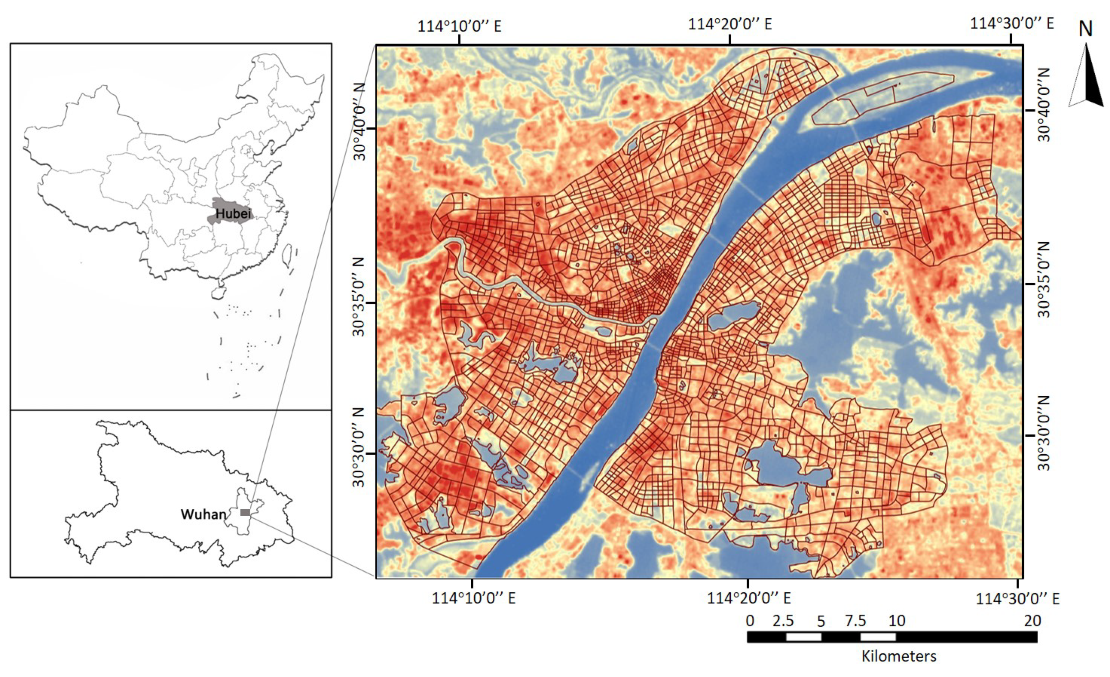
2.1. Study Area
2.2. Data Sets
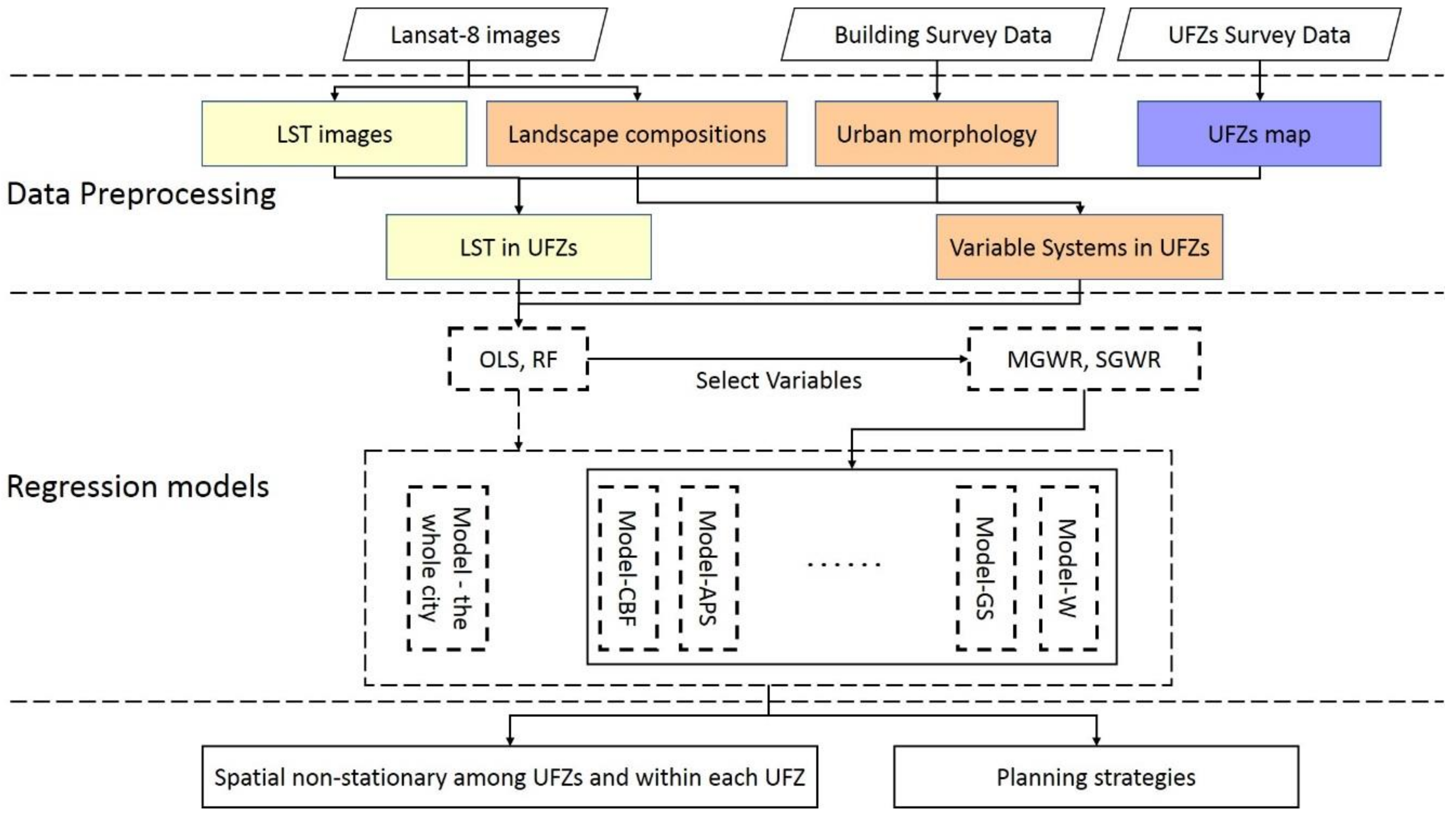
3. Methodology
3.1. The Retrieval of LST
3.2. The Selection of Landscape Indicators
3.3. Random Forest Regression Model
3.4. Geographic Weighted Regression Models
4. Results
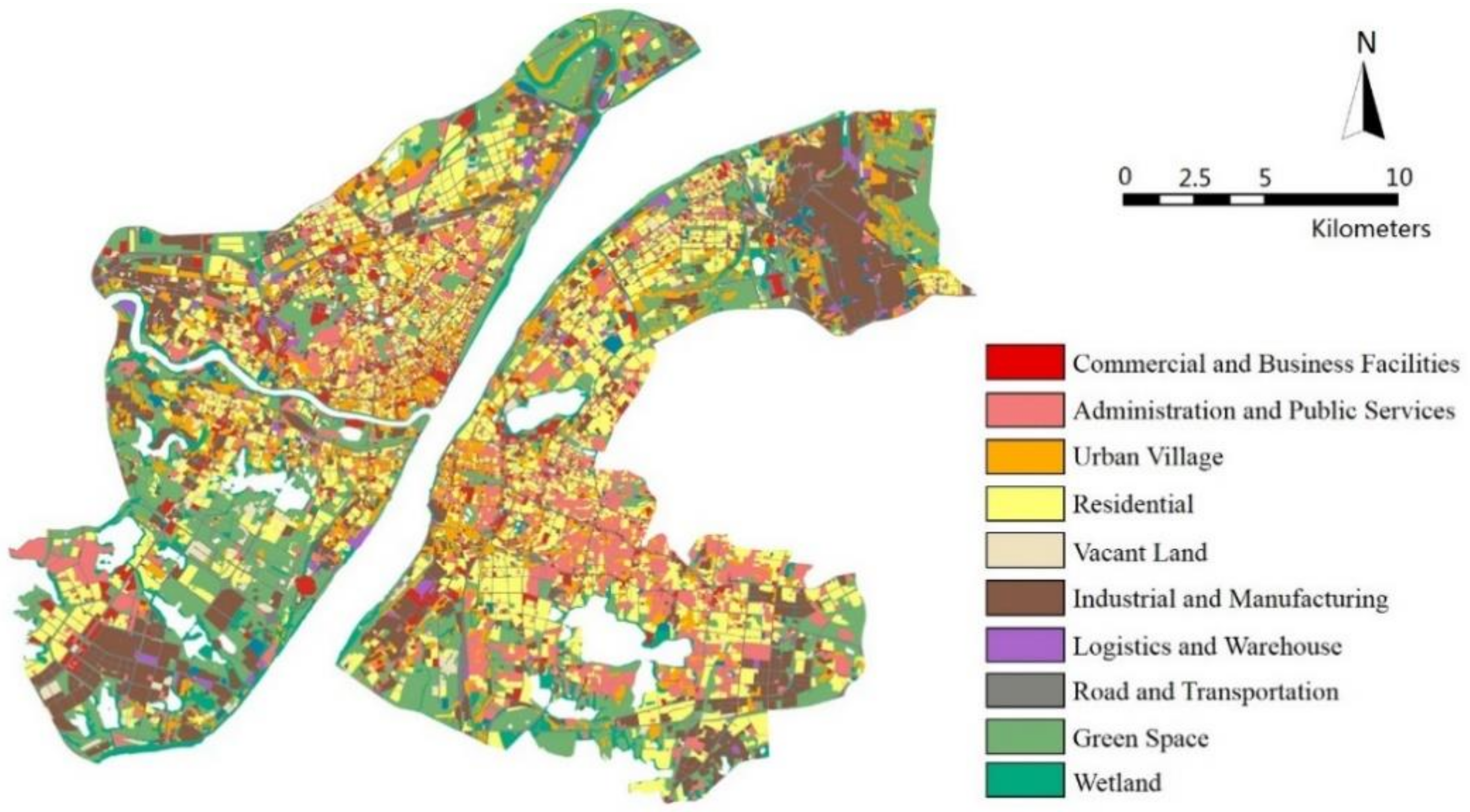
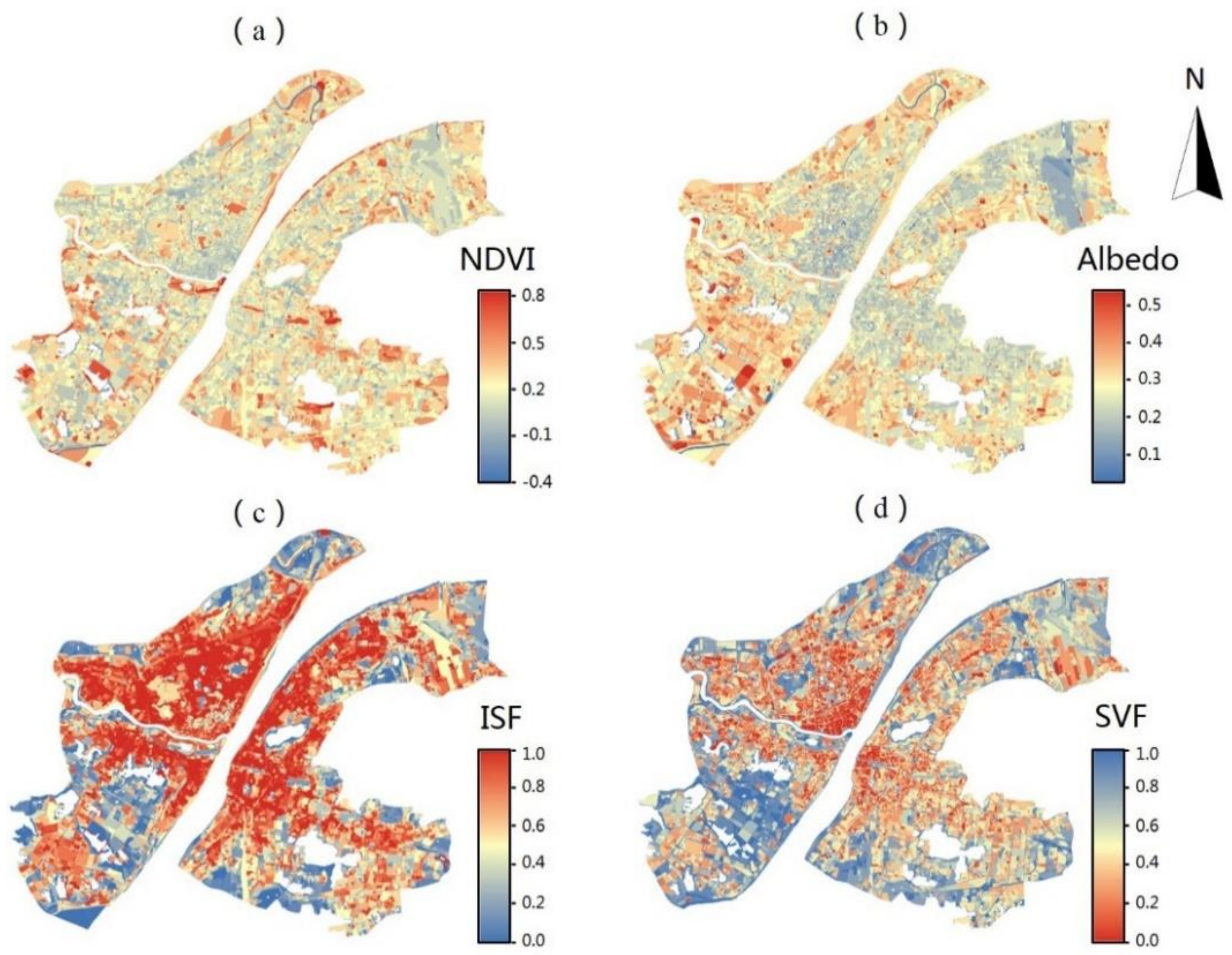
4.1. The Spatial Patterns of the LST and Landscape Indicators in Different Types of UFZs
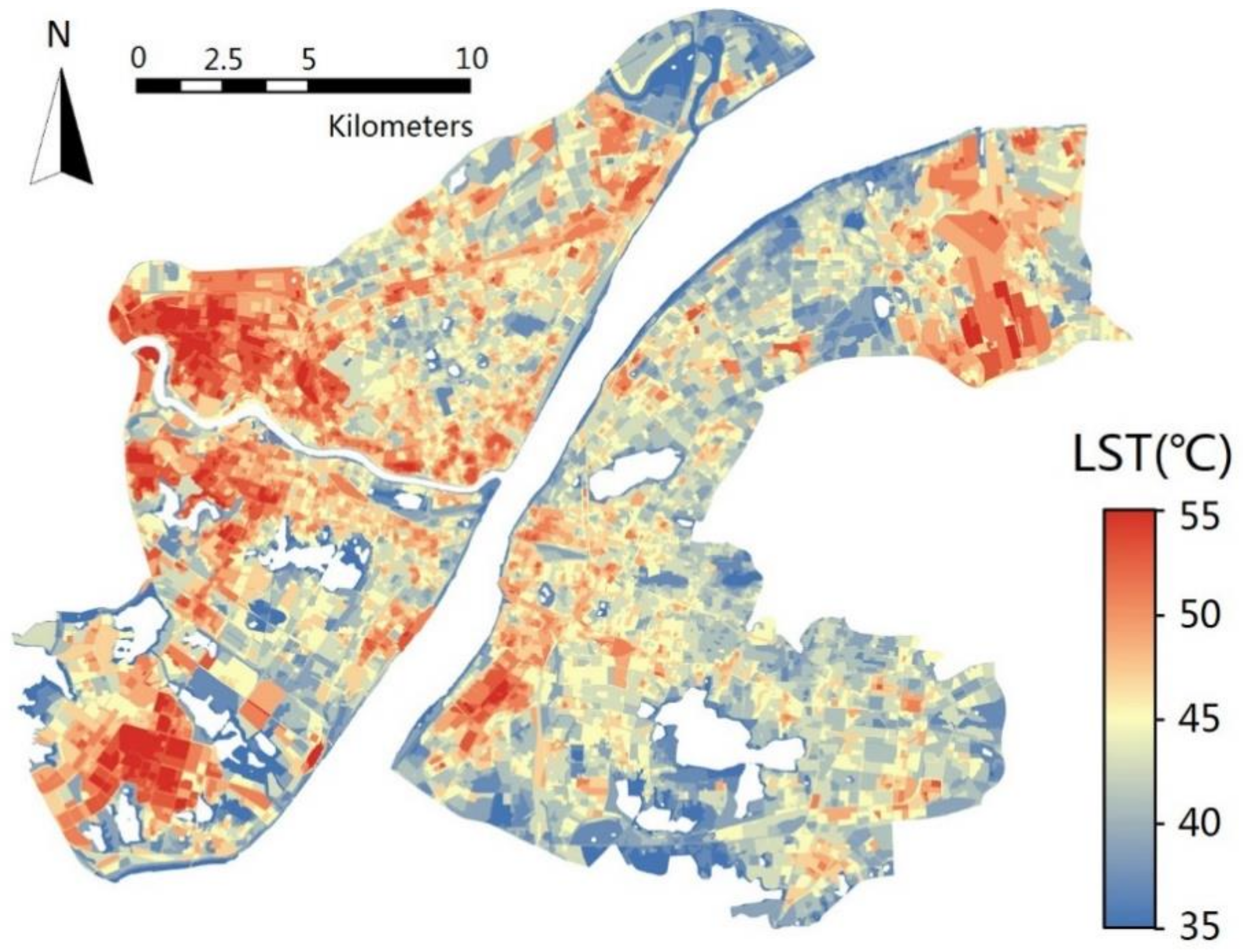
The Spatial Patterns of the LST in Different Types of UFZs
4.2. Regression Results Analysis
4.2.1. Performance Summary of the Global Regression Models
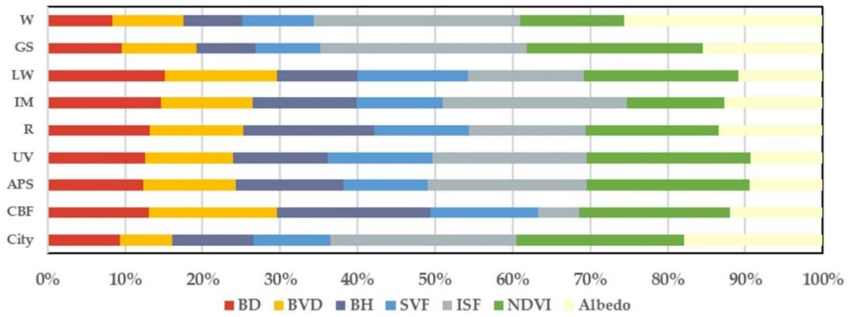
4.2.2. Performance Summary of the Random Forest Regression Models
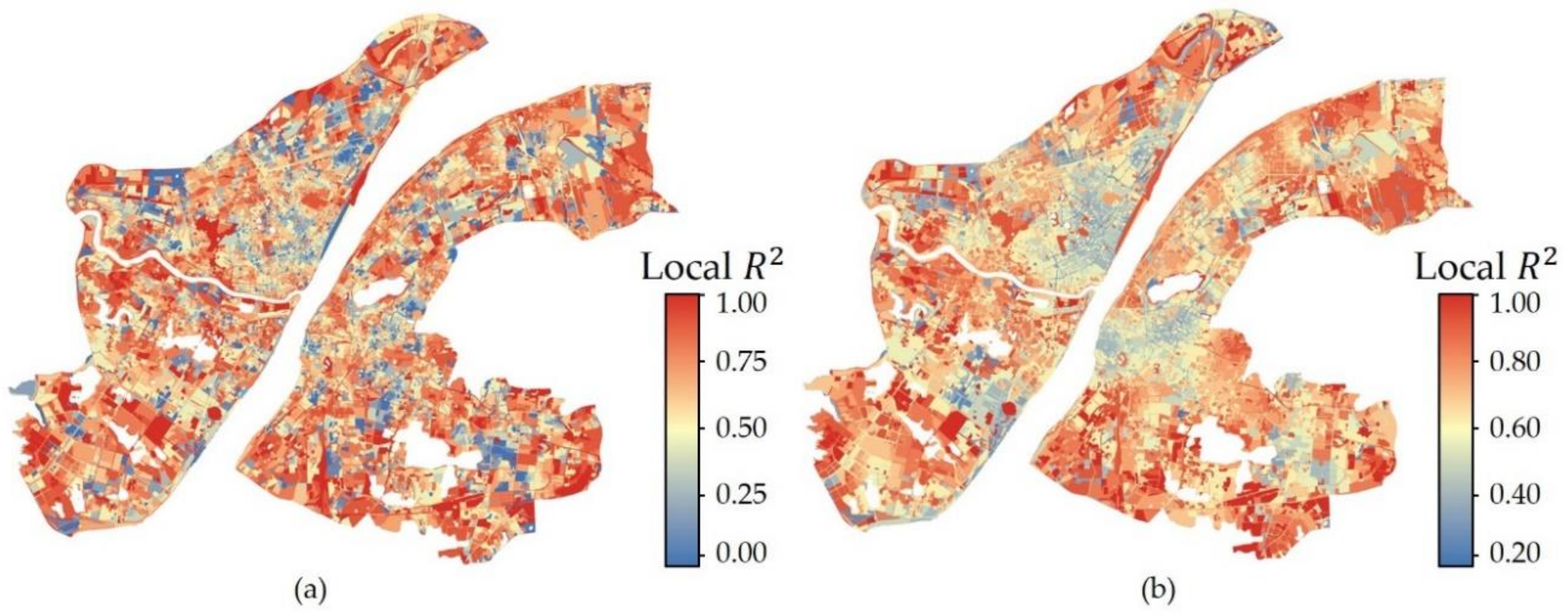
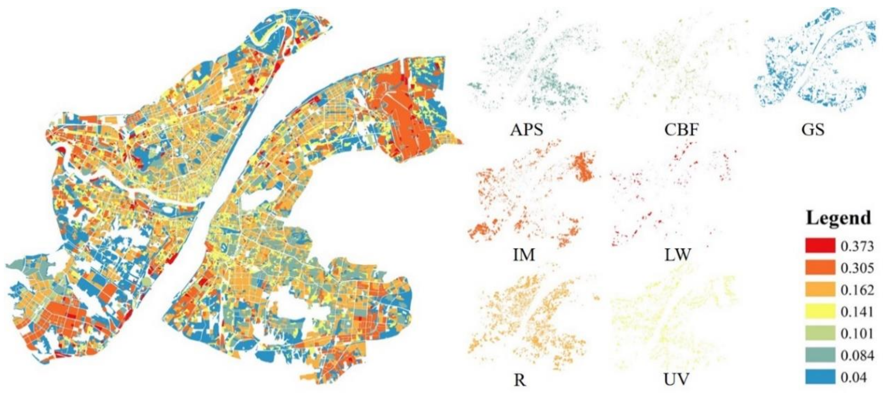
4.2.3. Non-Stationarity of the Three Geographically Weighted Regression Models
5. Discussion
5.1. Spatial Heterogeneity in Landscape-LST Relationship among UFZs and within Each-UFZ
5.2. Planning Strategies Based on the UFZs Unit
5.3. Limitation and Future Work
6. Conclusions
Author Contributions
Funding
Conflicts of Interest
Abbreviations
| LCZ | Local climate zones |
| UFZ | urban functional zone |
| LST | land surface temperature |
| OLS | ordinary least square regression |
| RF | random forest regression |
| SGWR | semi-parametric geographically weighted regression |
| MGWR | multiscale geographically weighted regression |
| 2D | two-dimensional |
| BD | building density |
| 3D | three-dimensional |
| BH | building height |
| BVD | building volume density |
| SVF | sky view factor |
| NDVI | normalized difference vegetation index |
| ISF | impervious surface fraction |
| R | Residential |
| UV | Urban village |
| APS | Administration and Public Services |
| CBF | Commercial and Business Facilities |
| IM | Industrial and Manufacturing |
| LW | Logistics and Warehouse |
| GWR | geographically weighted regression |
| GS | Green Space |
| RT | Road and Transportation |
| VL | Vacant Land |
| W | Wetland |
References
- Foley, J.A.; DeFries, R.; Asner, G.P.; Barford, C.; Bonan, G.; Carpenter, S.R.; Chapin, F.S.; Coe, M.T.; Daily, G.C.; Gibbs, H.K.; et al. Global Consequences of Land Use. Science 2005, 309, 570. [Google Scholar]
- Mora, C.; Spirandelli, D.; Franklin, E.C.; Lynham, J.; Kantar, M.B.; Miles, W.; Smith, C.Z.; Freel, K.; Moy, J.; Louis, L.V.; et al. Broad threat to humanity from cumulative climate hazards intensified by greenhouse gas emissions. Nat. Clim. Chang. 2018, 8, 1062–1071. [Google Scholar]
- Li, Y.; Schubert, S.; Kropp, J.P.; Rybski, D. On the influence of density and morphology on the Urban Heat Island intensity. Nat. Commun. 2020, 11, 2647. [Google Scholar] [PubMed]
- Oke, T.R.; Mills, G.; Voogt, J.A. Urban Climates; Cambridge University Press: Cambridge, UK, 2017. [Google Scholar]
- Grimm, N.B.; Faeth, S.H.; Golubiewski, N.E.; Redman, C.L.; Wu, J.; Bai, X.; Briggs, J.M. Global Change and the Ecology of Cities. Science 2008, 319, 756. [Google Scholar] [PubMed] [Green Version]
- Bastian, O.; Röder, M. Assessment of landscape change by land evaluation of past and present situation. Landsc. Urban Plan. 1998, 41, 171–182. [Google Scholar]
- Hirose, C.; Ikegaya, N.; Hagishima, A. Outdoor measurements of relationship between canopy flow and wall pressure distributions of a block within urban-like block array. Build. Environ. 2020, 176, 106881. [Google Scholar]
- He, B. Potentials of meteorological characteristics and synoptic conditions to mitigate urban heat island effects. Urban Clim. 2018, 24, 26–33. [Google Scholar]
- Oke, T.R. The energetic basis of the urban heat island. Q. J. R. Meteor. Soc. 1982, 108, 1–24. [Google Scholar]
- Weng, Q. Thermal infrared remote sensing for urban climate and environmental studies: Methods, applications, and trends. ISPRS J. Photogramm. Remote Sens. 2009, 64, 335–344. [Google Scholar]
- Liu, H.; Zhan, Q.; Yang, C.; Wang, J. The multi-timescale temporal patterns and dynamics of land surface temperature using Ensemble Empirical Mode Decomposition. Sci. Total Environ. 2019, 652, 243–255. [Google Scholar]
- Essa, W.; van der Kwast, J.; Verbeiren, B.; Batelaan, O. Downscaling of thermal images over urban areas using the land surface temperature—Impervious percentage relationship. Int. J. Appl. Earth Obs. 2013, 23, 95–108. [Google Scholar] [CrossRef]
- Yuan, F.; Bauer, M.E. Comparison of impervious surface area and normalized difference vegetation index as indicators of surface urban heat island effects in Landsat imagery. Remote Sens. Environ. 2007, 106, 375–386. [Google Scholar] [CrossRef]
- Song, J.; Chen, W.; Zhang, J.; Huang, K.; Hou, B.; Prishchepov, A.V. Effects of building density on land surface temperature in China: Spatial patterns and determinants. Landsc. Urban Plan. 2020, 198, 103794. [Google Scholar] [CrossRef]
- Lan, Y.; Zhan, Q. How do urban buildings impact summer air temperature? The effects of building configurations in space and time. Build. Environ. 2017, 125, 88–98. [Google Scholar] [CrossRef]
- Tran, D.X.; Pla, F.; Latorre-Carmona, P.; Myint, S.W.; Caetano, M.; Kieu, H.V. Characterizing the relationship between land use land cover change and land surface temperature. ISPRS J. Photogramm. Remote Sens. 2017, 124, 119–132. [Google Scholar] [CrossRef] [Green Version]
- Stewart, I.D. A systematic review and scientific critique of methodology in modern urban heat island literature. Int. J. Climatol. 2011, 31, 200–217. [Google Scholar] [CrossRef]
- Chang, C.; Li, M.; Chang, S. A preliminary study on the local cool-island intensity of Taipei city parks. Landsc. Urban Plan. 2007, 80, 386–395. [Google Scholar] [CrossRef]
- Su, Y.; Foody, G.M.; Cheng, K. Spatial non-stationarity in the relationships between land cover and surface temperature in an urban heat island and its impacts on thermally sensitive populations. Landsc. Urban Plan. 2012, 107, 172–180. [Google Scholar] [CrossRef]
- Tu, J.; Xia, Z. Examining spatially varying relationships between land use and water quality using geographically weighted regression I: Model design and evaluation. Sci. Total Environ. 2008, 407, 358–378. [Google Scholar] [CrossRef]
- Stone, B.; Vargo, J.; Habeeb, D. Managing climate change in cities: Will climate action plans work? Landsc. Urban Plan. 2012, 107, 263–271. [Google Scholar] [CrossRef]
- Stewart, I.D.; Oke, T.R. Local climate zones and urban climatic mapping. In The Urban Climatic Map: A Methodology for Sustainable Urban Planning; Ng, E., Ren, C., Eds.; Routledge: London, UK, 2015; pp. 397–401. [Google Scholar]
- Stewart, I.D.; Oke, T.R. Local Climate Zones for Urban Temperature Studies. Bull. Am. Meteorol. Soc. 2012, 93, 1879–1900. [Google Scholar] [CrossRef]
- Feng, Y.; Du, S.; Myint, S.W.; Shu, M. Do Urban Functional Zones Affect Land Surface Temperature Differently? A Case Study of Beijing, China. Remote Sens. 2019, 11, 1802. [Google Scholar] [CrossRef] [Green Version]
- Bechtel, B.; Demuzere, M.; Mills, G.; Zhan, W.; Sismanidis, P.; Small, C.; Voogt, J. SUHI analysis using Local Climate Zones—A comparison of 50 cities. Urban Clim. 2019, 28, 100451. [Google Scholar] [CrossRef]
- Yang, J.; Zhan, Y.; Xiao, X.; Xia, J.C.; Sun, W.; Li, X. Investigating the diversity of land surface temperature characteristics in different scale cities based on local climate zones. Urban Clim. 2020, 34, 100700. [Google Scholar] [CrossRef]
- Sun, R.; Lü, Y.; Chen, L.; Yang, L.; Chen, A. Assessing the stability of annual temperatures for different urban functional zones. Build. Environ. 2013, 65, 90–98. [Google Scholar] [CrossRef]
- Wu, Z.; Yao, L.; Ren, Y. Characterizing the spatial heterogeneity and controlling factors of land surface temperature clusters: A case study in Beijing. Build. Environ. 2020, 169, 106598. [Google Scholar] [CrossRef]
- Tian, G.; Wu, J.; Yang, Z. Spatial pattern of urban functions in the Beijing metropolitan region. Habitat Int. 2010, 34, 249–255. [Google Scholar] [CrossRef]
- Huang, X.; Wang, Y. Investigating the effects of 3D urban morphology on the surface urban heat island effect in urban functional zones by using high-resolution remote sensing data: A case study of Wuhan, Central China. ISPRS J. Photogramm. Remote Sens. 2019, 152, 119–131. [Google Scholar] [CrossRef]
- Zhang, X.; Du, S.; Du, S.; Liu, B. How do land-use patterns influence residential environment quality? A multiscale geographic survey in Beijing. Remote Sens. Environ. 2020, 249, 112014. [Google Scholar] [CrossRef]
- Yao, L.; Xu, Y.; Zhang, B. Effect of urban function and landscape structure on the urban heat island phenomenon in Beijing, China. Landsc. Ecol. Eng. 2019, 15, 379–390. [Google Scholar] [CrossRef]
- Liu, H.; Zhan, Q.; Gao, S.; Yang, C. Seasonal Variation of the Spatially Non-Stationary Association Between Land Surface Temperature and Urban Landscape. Remote Sens. 2019, 11, 1016. [Google Scholar] [CrossRef] [Green Version]
- Yin, C.; Yuan, M.; Lu, Y.; Huang, Y.; Liu, Y. Effects of urban form on the urban heat island effect based on spatial regression model. Sci. Total Environ. 2018, 634, 696–704. [Google Scholar] [CrossRef] [PubMed]
- Stewart, I.D.; Oke, T.R.; Krayenhoff, E.S. Evaluation of the ‘local climate zone’ scheme using temperature observations and model simulations. Int. J. Climatol. 2014, 34, 1062–1080. [Google Scholar] [CrossRef]
- Zhao, C.; Jensen, J.; Weng, Q.; Currit, N.; Weaver, R. Application of airborne remote sensing data on mapping local climate zones: Cases of three metropolitan areas of Texas, U.S. Comput. Environ. Urban Syst. 2019, 74, 175–193. [Google Scholar] [CrossRef]
- Sun, Y.; Gao, C.; Li, J.; Wang, R.; Liu, J. Quantifying the Effects of Urban Form on Land Surface Temperature in Subtropical High-Density Urban Areas Using Machine Learning. Remote Sens. 2019, 11, 959. [Google Scholar] [CrossRef] [Green Version]
- Zhao, C.; Weng, Q.; Hersperger, A.M. Characterizing the 3-D urban morphology transformation to understand urban-form dynamics: A case study of Austin, Texas, USA. Landsc. Urban Plan. 2020, 203, 103881. [Google Scholar] [CrossRef]
- Zhao, C.; Jensen, J.L.R.; Weng, Q.; Currit, N.; Weaver, R. Use of Local Climate Zones to investigate surface urban heat islands in Texas. GISci. Remote Sens. 2020, 57, 1083–1101. [Google Scholar] [CrossRef]
- Li, W.; Cao, Q.; Lang, K.; Wu, J. Linking potential heat source and sink to urban heat island: Heterogeneous effects of landscape pattern on land surface temperature. Sci. Total Environ. 2017, 586, 457–465. [Google Scholar] [CrossRef]
- Fotheringham, A.S.; Yang, W.; Kang, W. Multiscale Geographically Weighted Regression (MGWR). Ann. Am. Assoc. Geogr. 2017, 107, 1247–1265. [Google Scholar] [CrossRef]
- Zhao, C.; Jensen, J.; Weng, Q.; Weaver, R. A Geographically Weighted Regression Analysis of the Underlying Factors Related to the Surface Urban Heat Island Phenomenon. Remote Sens. 2018, 10, 1428. [Google Scholar] [CrossRef] [Green Version]
- Georgescu, M.; Morefield, P.E.; Bierwagen, B.G.; Weaver, C.P. Urban adaptation can roll back warming of emerging megapolitan regions. Proc. Natl. Acad. Sci. USA 2014, 111, 2909. [Google Scholar] [CrossRef] [PubMed] [Green Version]
- Buyantuyev, A.; Wu, J. Urban heat islands and landscape heterogeneity: Linking spatiotemporal variations in surface temperatures to land-cover and socioeconomic patterns. Landsc. Ecol. 2010, 25, 17–33. [Google Scholar] [CrossRef]
- McMaster, R.B.; Sheppard, E. Introduction: Scale and geographic inquiry. In Scale and Geographic Inquiry: Nature, Society, and Method; Wiley-Blackwell: Hoboken, NJ, USA, 2004. [Google Scholar]
- Yang, C.; Zhan, Q.; Lv, Y.; Liu, H. Downscaling Land Surface Temperature Using Multiscale Geographically Weighted Regression over Heterogeneous Landscapes in Wuhan, China. IEEE J. Sel. Top. Appl. Earth Obs. Remote Sens. 2019, 12, 5213–5222. [Google Scholar] [CrossRef]
- Mirchooli, F.; Kiani-Harchegani, M.; Khaledi Darvishan, A.; Falahatkar, S.; Sadeghi, S.H. Spatial distribution dependency of soil organic carbon content to important environmental variables. Ecol. Indic. 2020, 116, 106473. [Google Scholar] [CrossRef]
- Grimm, R.; Behrens, T.; Märker, M.; Elsenbeer, H. Soil organic carbon concentrations and stocks on Barro Colorado Island—Digital soil mapping using Random Forests analysis. Geoderma 2008, 146, 102–113. [Google Scholar] [CrossRef]
- Sobrino, J.A.; Jiménez-Muñoz, J.C.; Paolini, L. Land surface temperature retrieval from LANDSAT TM 5. Remote Sens. Environ. 2004, 90, 434–440. [Google Scholar] [CrossRef]
- Yu, X.; Guo, X.; Wu, Z. Land Surface Temperature Retrieval from Landsat 8 TIRS—Comparison between Radiative Transfer Equation-Based Method, Split Window Algorithm and Single Channel Method. Remote Sens. 2014, 6, 9829–9852. [Google Scholar] [CrossRef] [Green Version]
- Barsi, J.A.; Schott, J.R.; Palluconi, F.D.; Helder, D.L.; Hook, S.J.; Markham, B.L.; Chander, G.; O’Donnell, E.M. Landsat TM and ETM+ thermal band calibration. Can. J. Remote Sens. 2003, 29, 141–153. [Google Scholar] [CrossRef]
- Peng, J.; Jia, J.; Liu, Y.; Li, H.; Wu, J. Seasonal contrast of the dominant factors for spatial distribution of land surface temperature in urban areas. Remote Sens. Environ. 2018, 215, 255–267. [Google Scholar] [CrossRef]
- Chen, X.; Zhao, H.; Li, P.; Yin, Z. Remote sensing image-based analysis of the relationship between urban heat island and land use/cover changes. Remote Sens. Environ. 2006, 104, 133–146. [Google Scholar] [CrossRef]
- Haashemi, S.; Weng, Q.; Darvishi, A.; Alavipanah, S.K. Seasonal Variations of the Surface Urban Heat Island in a Semi-Arid City. Remote Sens. 2016, 8, 352. [Google Scholar] [CrossRef] [Green Version]
- Gong, P.; Li, X.; Zhang, W. 40-Year (1978–2017) human settlement changes in China reflected by impervious surfaces from satellite remote sensing. Sci. Bull. 2019, 64, 756–763. [Google Scholar] [CrossRef] [Green Version]
- Sun, R.; Lü, Y.; Yang, X.; Chen, L. Understanding the variability of urban heat islands from local background climate and urbanization. J. Clean. Prod. 2019, 208, 743–752. [Google Scholar] [CrossRef]
- Breiman, L. Random Forests. Mach. Learn. 2001, 45, 5–32. [Google Scholar] [CrossRef] [Green Version]
- Xu, Y.; Knudby, A.; Shen, Y.; Liu, Y. Mapping Monthly Air Temperature in the Tibetan Plateau From MODIS Data Based on Machine Learning Methods. IEEE J. Sel. Top. Appl. Earth Obs. Remote Sens. 2018, 11, 345–354. [Google Scholar] [CrossRef]
- Genuer, R.; Poggi, J.; Tuleau-Malot, C. Variable selection using random forests. Pattern Recogn. Lett. 2010, 31, 2225–2236. [Google Scholar] [CrossRef] [Green Version]
- Fotheringham, A.S.; Brunsdon, C.; Charlton, M. Geographically Weighted Regression: The Analysis of Spatially Varying Relationships; John Wiley & Sons: Hoboken, NJ, USA, 2003. [Google Scholar]
- Nakaya, T.; Fotheringham, S.; Charlton, M.; Brunsdon, C. Semiparametric Geographically Weighted Generalised Linear Modelling in GWR 4.0. Geocomputation 2009. [Google Scholar]
- Li, C.; Zhao, J.; Xu, Y. Examining spatiotemporally varying effects of urban expansion and the underlying driving factors. Sustain. Cities Soc. 2017, 28, 307–320. [Google Scholar] [CrossRef]
- Yang, J.; Wang, Y.; Xiu, C.; Xiao, X.; Xia, J.; Jin, C. Optimizing local climate zones to mitigate urban heat island effect in human settlements. J. Clean. Prod. 2020, 275, 123767. [Google Scholar] [CrossRef]
- Sun, R.; Wang, Y.; Chen, L. A distributed model for quantifying temporal-spatial patterns of anthropogenic heat based on energy consumption. J. Clean. Prod. 2018, 170, 601–609. [Google Scholar] [CrossRef]
- He, C.; Zhou, L.; Yao, Y.; Ma, W.; Kinney, P.L. Estimating spatial effects of anthropogenic heat emissions upon the urban thermal environment in an urban agglomeration area in East China. Sustain. Cities Soc. 2020, 57, 102046. [Google Scholar] [CrossRef]
- Zhang, C.; Yang, Y. Modeling the spatial variations in anthropogenic factors of soil heavy metal accumulation by geographically weighted logistic regression. Sci. Total Environ. 2020, 717, 137096. [Google Scholar] [CrossRef] [PubMed]
- Quah, A.K.L.; Roth, M. Diurnal and weekly variation of anthropogenic heat emissions in a tropical city, Singapore. Atmos. Environ. 2012, 46, 92–103. [Google Scholar] [CrossRef]
- Shafran-Nathan, R.; Yuval; Broday, D.M. Impacts of Personal Mobility and Diurnal Concentration Variability on Exposure Misclassification to Ambient Pollutants. Environ. Sci. Technol. 2018, 52, 3520–3526. [Google Scholar] [CrossRef] [PubMed]
- Sun, F.; Liu, M.; Wang, Y.; Wang, H.; Che, Y. The effects of 3D architectural patterns on the urban surface temperature at a neighborhood scale: Relative contributions and marginal effects. J. Clean. Prod. 2020, 258, 120706. [Google Scholar] [CrossRef]
- Jamei, E.; Rajagopalan, P. Urban development and pedestrian thermal comfort in Melbourne. Sol. Energy 2017, 144, 681–698. [Google Scholar] [CrossRef]
- Li, J.; Song, C.; Cao, L.; Zhu, F.; Meng, X.; Wu, J. Impacts of landscape structure on surface urban heat islands: A case study of Shanghai, China. Remote Sens. Environ. 2011, 115, 3249–3263. [Google Scholar] [CrossRef]
- Chun, B.; Guldmann, J.M. Spatial statistical analysis and simulation of the urban heat island in high-density central cities. Landsc. Urban Plan. 2014, 125, 76–88. [Google Scholar] [CrossRef]
- Wu, Z.; Wang, Y.; Kong, F.; Sun, R.; Chen, L.; Zhan, W. Analysis of the thermal characteristics of selected urban surfaces in a typical residential area based on infrared thermography. Acta Ecol. Sin. 2016, 36, 5421–5431. [Google Scholar]
- Jia, W.; Zhao, S. Trends and drivers of land surface temperature along the urban-rural gradients in the largest urban agglomeration of China. Sci. Total Environ. 2020, 711, 134579. [Google Scholar] [CrossRef]
- Harman, I.N.; Best, M.J.; Belcher, S.E. Radiative Exchange in an Urban Street Canyon. Bound. Lay. Meteorol. 2004, 110, 301–316. [Google Scholar] [CrossRef]
- Rosenfeld, A.H.; Akbari, H.; Bretz, S.; Fishman, B.L.; Kurn, D.M.; Sailor, D.; Taha, H. Mitigation of urban heat islands: Materials, utility programs, updates. Energy Build. 1995, 22, 255–265. [Google Scholar] [CrossRef]
- He, B.; Zhao, Z.; Shen, L.; Wang, H.; Li, L. An approach to examining performances of cool/hot sources in mitigating/enhancing land surface temperature under different temperature backgrounds based on landsat 8 image. Sustain. Cities Soc. 2019, 44, 416–427. [Google Scholar] [CrossRef]
- Huang, F.; Zhan, W.; Wang, Z.; Voogt, J.; Hu, L.; Quan, J.; Liu, C.; Zhang, N.; Lai, J. Satellite identification of atmospheric-surface-subsurface urban heat islands under clear sky. Remote Sens. Environ. 2020, 250, 112039. [Google Scholar] [CrossRef]
- Ma, W.; Chen, Y.; Zhan, W.; Zhou, J. Thermal anisotropy model for simulated three dimensional urban targets. J. Remote Sens. 2013, 17, 62–76. [Google Scholar]


| Indicators | Description | Range |
|---|---|---|
| Landscape composition indicators retrieved from Landsat images | ||
| NDVI | Growth status, abundance, and coverage of vegetation, calculated as | [−1,1] |
| (ρ(NIR) − ρ(Red))/(ρ(NIR) + ρ(Red)) | ||
| albedo | Overall reflectance in all directions | [0,1] |
| Landscape composition indicators retrieved from open-source datasets | ||
| ISF | Fraction of impervious surface | [0,1] |
| Morphology indicators retrieved from building survey data | ||
| BD | The total area of building divided by the pixel area | [0,1] |
| BH | The area averaged building height | [0,max] |
| BVD | A 3D indicator calculated as the building volume divided by the pixel area | [0,max] |
| SVF | The fraction of sky visibility at a given point | [0,1] |
| UFZs Category | The Number of Zones | Average Area/m2 | Area Percentage | Average LST/°C | LST STD/°C |
|---|---|---|---|---|---|
| Commercial and Business Facilities (CBF) | 2201 | 10,304 | 4.45% | 47.76 | 2.13 |
| Administration and Public Services (APS) | 3555 | 17,796 | 12.43% | 46.34 | 2.04 |
| Urban Village (UV) | 2557 | 17,949 | 9.02% | 47.50 | 2.13 |
| Residential (R) | 3920 | 25,016 | 19.26% | 45.75 | 1.88 |
| Vacant Land (VL) | 1130 | 21,689 | 4.81% | 46.89 | 2.04 |
| Industrial and Manufacturing (IM) | 2278 | 31,116 | 13.92% | 48.88 | 2.52 |
| Logistics and Warehouse (LW) | 353 | 26,240 | 1.82% | 48.70 | 2.33 |
| Road and Transportation (RT) | 4223 | 12,989 | 10.78% | 46.70 | 2.25 |
| Green Space (GS) | 2376 | 39,120 | 18.26% | 43.80 | 2.53 |
| Wetland (W) | 704 | 37,959 | 5.25% | 41.61 | 2.82 |
| Function | CBF | APS | UV | R | VL | IM | LW | RT | GS | W | |
|---|---|---|---|---|---|---|---|---|---|---|---|
| BD/m2 | mean | 0.37 | 0.20 | 0.37 | 0.26 | 0.02 | 0.31 | 0.24 | 0.06 | 0.02 | 0.01 |
| std | 0.17 | 0.09 | 0.14 | 0.05 | 0.02 | 0.15 | 0.17 | 0.07 | 0.02 | 0.01 | |
| BVD/m3 | mean | 4.84 | 2.30 | 3.37 | 5.72 | 0.19 | 1.62 | 1.19 | 0.59 | 0.14 | 0.05 |
| std | 3.64 | 1.42 | 1.66 | 1.33 | 0.28 | 0.89 | 0.92 | 0.77 | 0.17 | 0.06 | |
| BH/m | mean | 12.94 | 11.37 | 9.20 | 23.78 | 6.01 | 5.21 | 4.90 | 7.27 | 6.67 | 5.77 |
| std | 9.31 | 4.66 | 3.20 | 5.89 | 5.58 | 2.52 | 2.32 | 5.89 | 4.01 | 3.36 | |
| SVF | mean | 0.54 | 0.70 | 0.48 | 0.53 | 0.96 | 0.64 | 0.71 | 0.95 | 0.96 | 0.98 |
| std | 0.18 | 0.13 | 0.18 | 0.08 | 0.04 | 0.16 | 0.19 | 0.12 | 0.03 | 0.02 | |
| ISF | mean | 0.84 | 0.70 | 0.81 | 0.81 | 0.59 | 0.75 | 0.80 | 0.82 | 0.33 | 0.26 |
| std | 0.17 | 0.23 | 0.17 | 0.10 | 0.29 | 0.19 | 0.18 | 0.24 | 0.23 | 0.20 | |
| NDVI | mean | 0.20 | 0.36 | 0.26 | 0.31 | 0.23 | 0.25 | 0.25 | 0.29 | 0.48 | 0.37 |
| std | 0.09 | 0.09 | 0.09 | 0.04 | 0.08 | 0.08 | 0.09 | 0.11 | 0.11 | 0.20 | |
| Albedo | mean | 0.20 | 0.18 | 0.17 | 0.16 | 0.22 | 0.20 | 0.20 | 0.18 | 0.19 | 0.16 |
| std | 0.04 | 0.02 | 0.02 | 0.01 | 0.02 | 0.05 | 0.04 | 0.03 | 0.02 | 0.05 | |
| City | CBF | APS | UV | R | VL | IM | LW | RST | GS | W | |
|---|---|---|---|---|---|---|---|---|---|---|---|
| OLS | 0.40 | 0.26 | 0.31 | 0.41 | 0.33 | 0.06 | 0.31 | 0.31 | 0.21 | 0.33 | 0.29 |
| RF | 0.45 | 0.28 | 0.32 | 0.42 | 0.35 | 0.05 | 0.34 | 0.28 | 0.20 | 0.38 | 0.37 |
| CBF | APS | UV | R | IM | LW | GS | W | ||
|---|---|---|---|---|---|---|---|---|---|
| GWR | R2 | 0.65 | 0.65 | 0.71 | 0.71 | 0.76 | 0.54 | 0.67 | 0.67 |
| AICC | 4322.82 | 6267.77 | 4450.93 | 7155.12 | 3694.50 | 618.97 | 5096.00 | 1405.31 | |
| RSS | 571.37 | 858.97 | 569.72 | 1058.59 | 389.79 | 92.02 | 625.58 | 161.62 | |
| SGWR | R2 | 0.77 | 0.73 | 0.82 | 0.76 | 0.79 | 0.58 | 0.71 | 0.66 |
| AICC | 4047.80 | 5589.98 | 3949.39 | 6771.26 | 3181.71 | 550.22 | 4741.73 | 1321.99 | |
| RSS | 502.37 | 595.65 | 378.35 | 796.63 | 372.44 | 89.31 | 513.78 | 152.71 | |
| MGWR | R2 | 0.81 | 0.81 | 0.84 | 0.82 | 0.85 | 0.76 | 0.78 | 0.76 |
| AICC | 3582.77 | 5244.34 | 3597.96 | 9541.57 | 3041.07 | 545.31 | 3853.85 | 1269.37 | |
| RSS | 303.14 | 475.57 | 307.35 | 526.68 | 248.89 | 71.35 | 381.26 | 130.22 |
| BD | BVD | BH | SVF | ISF | NDVI | Albedo | ||
|---|---|---|---|---|---|---|---|---|
| CBF | MGWR | 0.097 | −0.112 | −0.129 | −0.092 | 0.069 | −0.15 | 0.002 |
| SGWR | 0.101 | −0.111 | −0.141 | −0.09 | 0.071 | −0.161 | 0.003 | |
| APS | MGWR | 0.072 | −0.104 | −0.066 | −0.032 | 0.157 | −0.203 | −0.011 |
| SGWR | 0.084 | −0.124 | −0.068 | −0.05 | 0.192 | −0.214 | −0.01 | |
| UV | MGWR | 0.14 | −0.114 | −0.059 | −0.101 | 0.125 | −0.202 | p < 0.05 |
| SGWR | 0.141 | −0.121 | −0.051 | −0.107 | 0.143 | −0.201 | ||
| R | MGWR | 0.16 | −0.14 | −0.11 | −0.069 | 0.123 | −0.181 | 0.051 |
| SGWR | 0.162 | −0.147 | −0.124 | −0.083 | 0.134 | −0.186 | 0.049 | |
| IM | MGWR | 0.305 | −0.189 | p < 0.05 | p < 0.05 | 0.153 | −0.107 | −0.018 |
| SGWR | 0.305 | −0.171 | 0.164 | −0.119 | −0.025 | |||
| LW | MGWR | 0.339 | −0.146 | p < 0.05 | p < 0.05 | 0.189 | −0.276 | −0.06 |
| SGWR | 0.373 | −0.191 | 0.225 | −0.287 | −0.04 | |||
| GS | MGWR | 0.03 | p < 0.05 | −0.043 | −0.067 | 0.282 | −0.267 | 0.174 |
| SGWR | 0.04 | −0.053 | −0.06 | 0.315 | −0.261 | 0.168 | ||
| W | MGWR | p < 0.05 | p < 0.05 | p < 0.05 | p < 0.05 | 0.3 | −0.058 | 0.306 |
| SGWR | 0.375 | −0.055 | 0.348 |
| CBF | APS | UV | R | IM | LW | GS | W | ||
|---|---|---|---|---|---|---|---|---|---|
| Intercept | GWR | 996.64 | 847.18 | 1024.88 | 997.24 | 847.72 | 3156.730 | 1042.39 | 1277.92 |
| SGWR | 558.34 | 341.74 | 369.73 | 567.27 | 395.32 | 1711 | 682.05 | 891.66 | |
| MGWR | 221.77 | 228.33 | 259.64 | 201.61 | 274.07 | 1277.31 | 340.66 | 631.03 | |
| BD | GWR | 996.64 | 847.18 | 1024.88 | 997.24 | 847.72 | 3156.730 | 1042.39 | p > 0.05 |
| SGWR | global | global | global | global | global | global | global | ||
| MGWR | 76,258.54 | 77,360.32 | 74,474.13 | 77,866.42 | 2402.03 | 34,814.55 | 79,683.88 | ||
| BVD | GWR | 996.64 | 847.18 | 1024.88 | 997.24 | 847.72 | 3156.730 | 1042.39 | p > 0.05 |
| SGWR | global | global | global | 567.27 | global | global | global | ||
| MGWR | 8090.44 | 77,360.32 | 74,474.13 | 77,866.42 | 3150.17 | 70,975.55 | 2237.86 | ||
| BH | GWR | 996.64 | 847.18 | 1024.88 | 997.24 | p > 0.05 | p > 0.05 | 1042.39 | p > 0.05 |
| SGWR | global | global | global | global | global | ||||
| MGWR | 76,258.54 | 77,360.32 | 74,474.13 | 7833.11 | 79,683.88 | ||||
| SVF | GWR | 996.64 | 847.18 | 1024.88 | 997.24 | p > 0.05 | p > 0.05 | 1042.39 | p > 0.05 |
| SGWR | global | global | global | global | global | ||||
| MGWR | 76,258.54 | 77,360.32 | 5292.86 | 13,689.35 | 79,683.88 | ||||
| ISF | GWR | 996.64 | 847.18 | 1024.88 | 997.24 | 847.72 | 3156.730 | 1042.39 | 1277.92 |
| SGWR | global | 341.74 | 369.73 | 567.27 | global | global | 682.05 | global | |
| MGWR | 76,258.54 | 5085.64 | 2318.58 | 77,866.42 | 78,630.13 | 3516.16 | 807.47 | 2301.5 | |
| NDVI | GWR | 996.64 | 847.18 | 1024.88 | 997.24 | 847.72 | 3156.730 | 1042.39 | 1277.92 |
| SGWR | 558.34 | global | global | 567.27 | global | global | 682.05 | global | |
| MGWR | 76,258.54 | 77,360.32 | 7796.52 | 2129.01 | 5596.41 | 7144.02 | 1310.45 | 78,682.86 | |
| albedo | GWR | 996.64 | 847.18 | p > 0.05 | 997.24 | 847.72 | 3156.730 | 1042.39 | 1277.92 |
| SGWR | 558.34 | global | 567.27 | global | global | 682.05 | 891.66 | ||
| MGWR | 76,258.54 | 77,360.32 | 77,866.42 | 5116.48 | 70,975.55 | 1196.87 | 2214.13 |
Publisher’s Note: MDPI stays neutral with regard to jurisdictional claims in published maps and institutional affiliations. |
© 2020 by the authors. Licensee MDPI, Basel, Switzerland. This article is an open access article distributed under the terms and conditions of the Creative Commons Attribution (CC BY) license (http://creativecommons.org/licenses/by/4.0/).
Share and Cite
Gao, S.; Zhan, Q.; Yang, C.; Liu, H. The Diversified Impacts of Urban Morphology on Land Surface Temperature among Urban Functional Zones. Int. J. Environ. Res. Public Health 2020, 17, 9578. https://0-doi-org.brum.beds.ac.uk/10.3390/ijerph17249578
Gao S, Zhan Q, Yang C, Liu H. The Diversified Impacts of Urban Morphology on Land Surface Temperature among Urban Functional Zones. International Journal of Environmental Research and Public Health. 2020; 17(24):9578. https://0-doi-org.brum.beds.ac.uk/10.3390/ijerph17249578
Chicago/Turabian StyleGao, Sihang, Qingming Zhan, Chen Yang, and Huimin Liu. 2020. "The Diversified Impacts of Urban Morphology on Land Surface Temperature among Urban Functional Zones" International Journal of Environmental Research and Public Health 17, no. 24: 9578. https://0-doi-org.brum.beds.ac.uk/10.3390/ijerph17249578