Spatio-Temporal Variations of Satellite-Based PM2.5 Concentrations and Its Determinants in Xinjiang, Northwest of China


Abstract
:1. Introduction
2. Materials and Methods
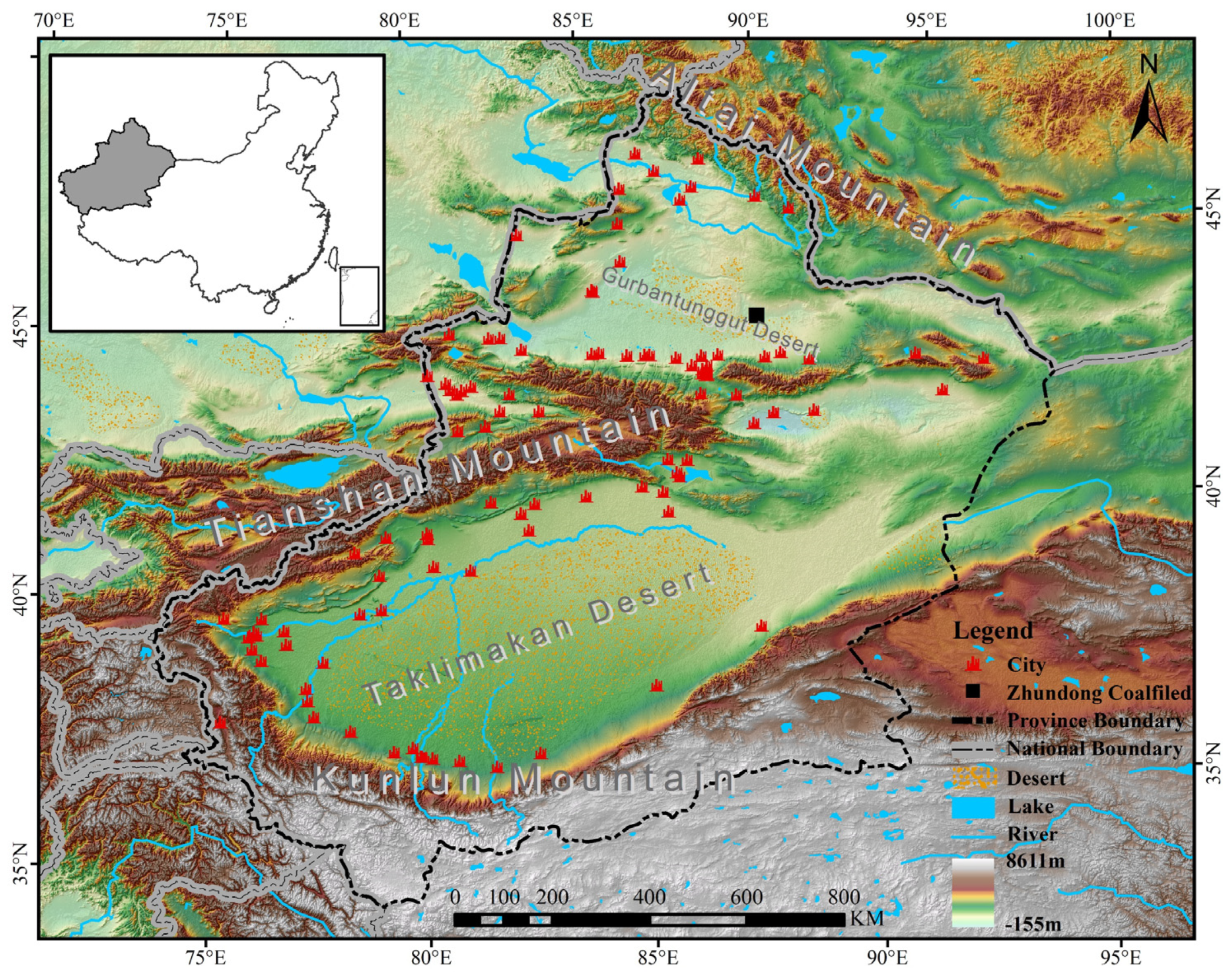
2.1. Study Area
2.2. Data Source
2.3. Method
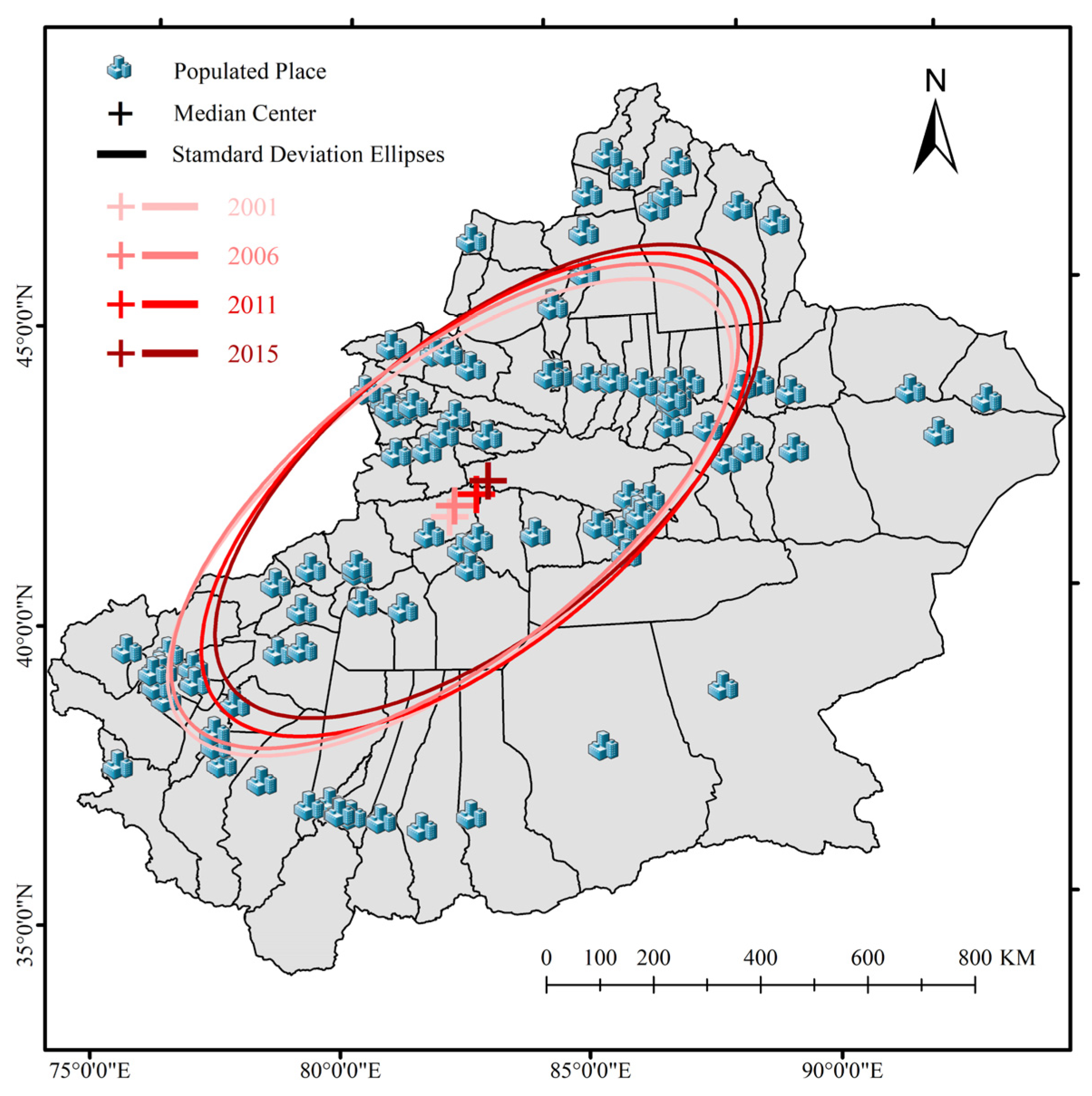
2.3.1. Standard Deviational Ellipse Analysis
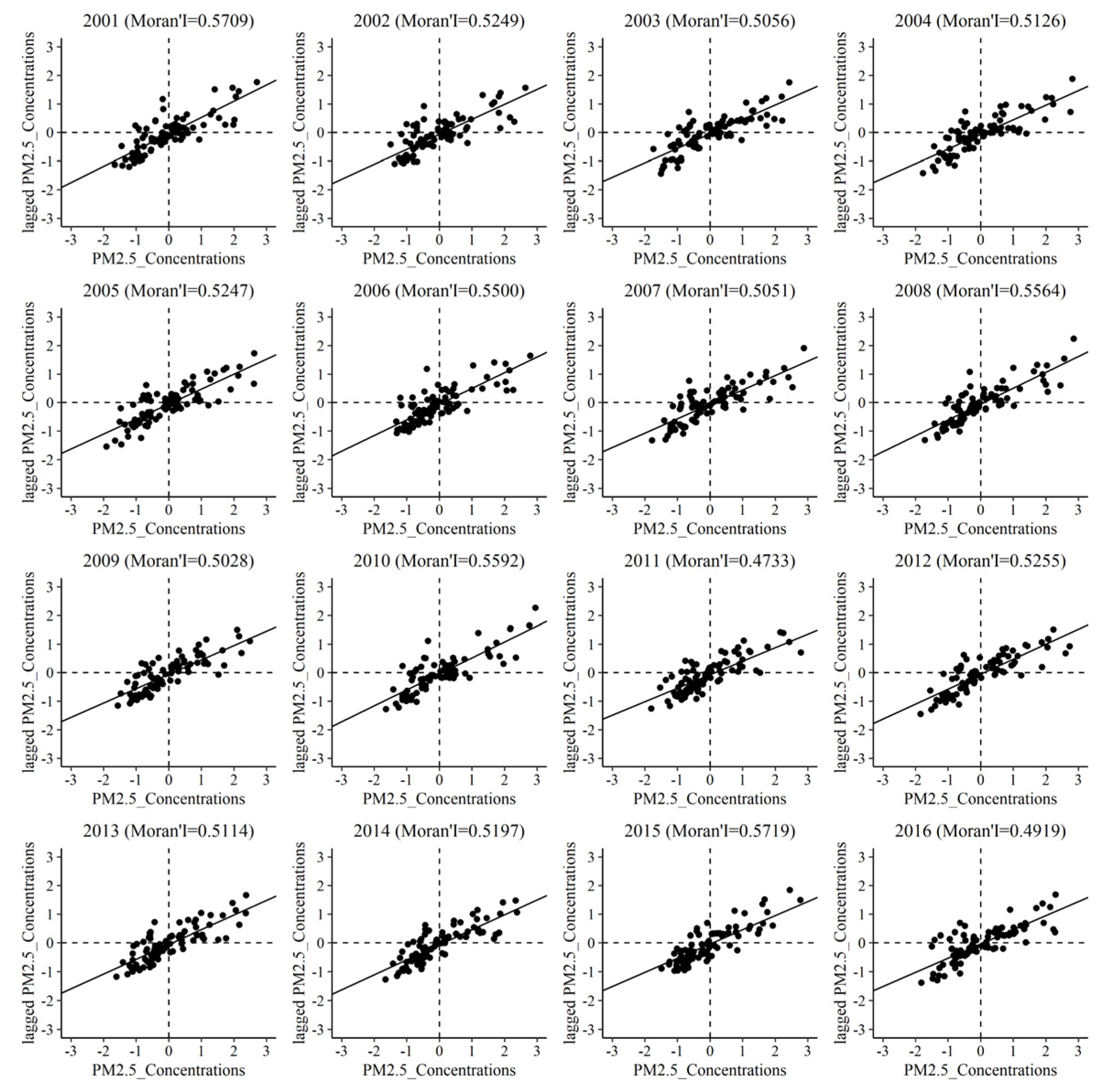
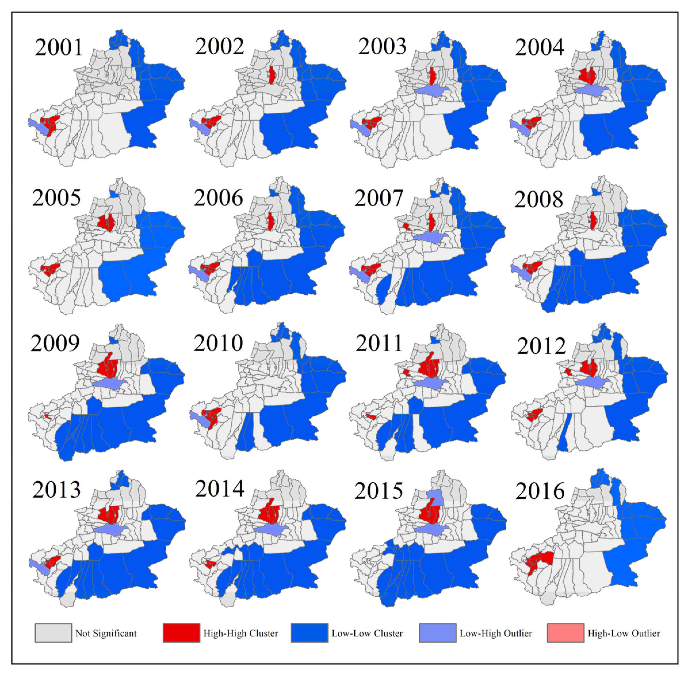
2.3.2. Spatial Autocorrelation Statistics
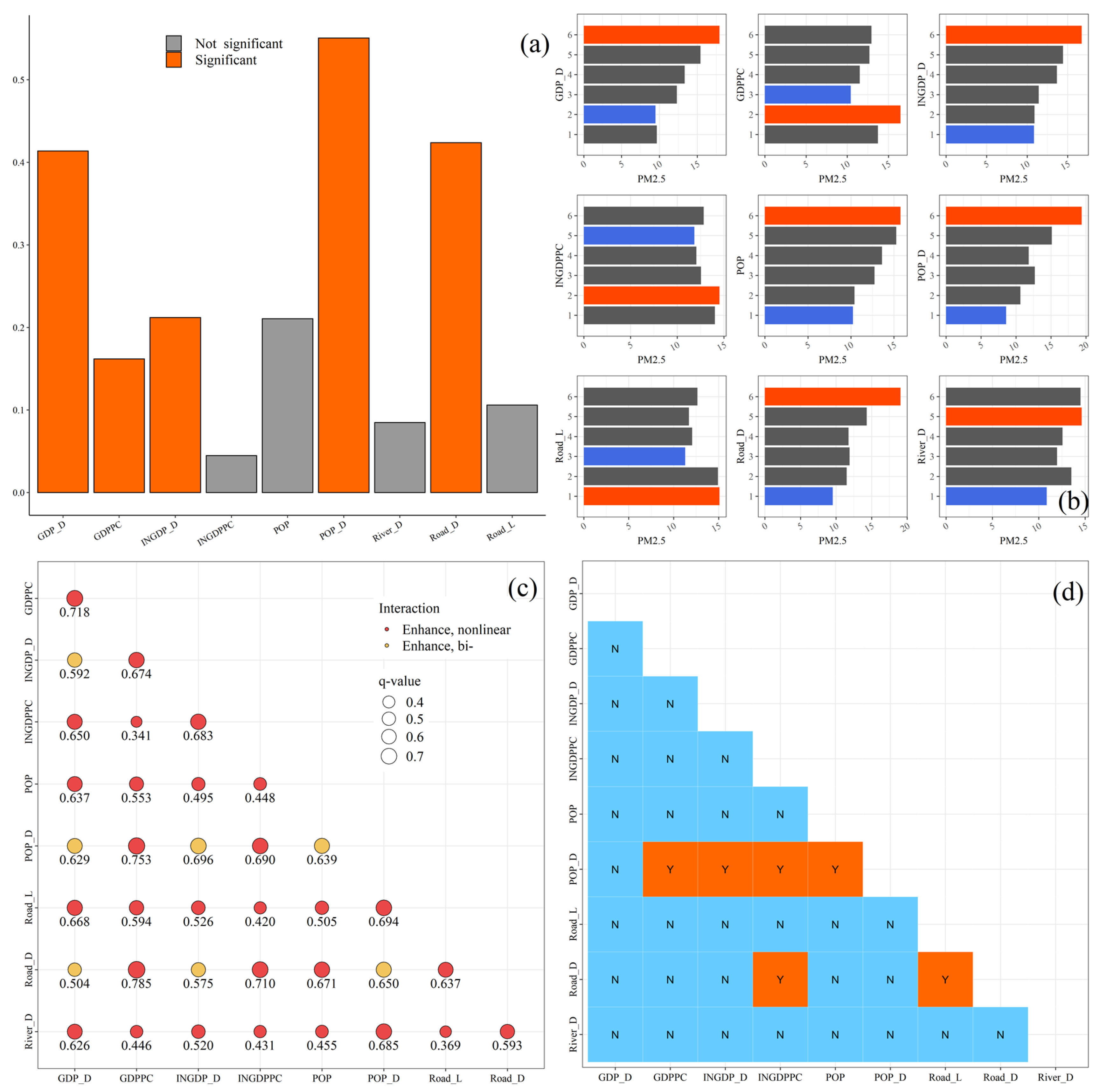
2.3.3. Geographical Detector Method
- (1)
- The factor detector calculates the determinant power of an explanatory variable X of Y, which is the q value we mentioned above.
- (2)
- The risk detector maps the average value of response variable in each stratum (zone). It can be used to compare the difference of average PM2.5 concentration values between sub-regions.
- (3)
- The interaction detector can reveal the interactive effect of X1 and X2 on Y. In other words, that is the relationship among q(X1), q(X2), and q(X1∩X2).
- (4)
- The ecological detector identifies the statistic difference of the impacts between X1 and X2. It can show the relative importance between these two factors.
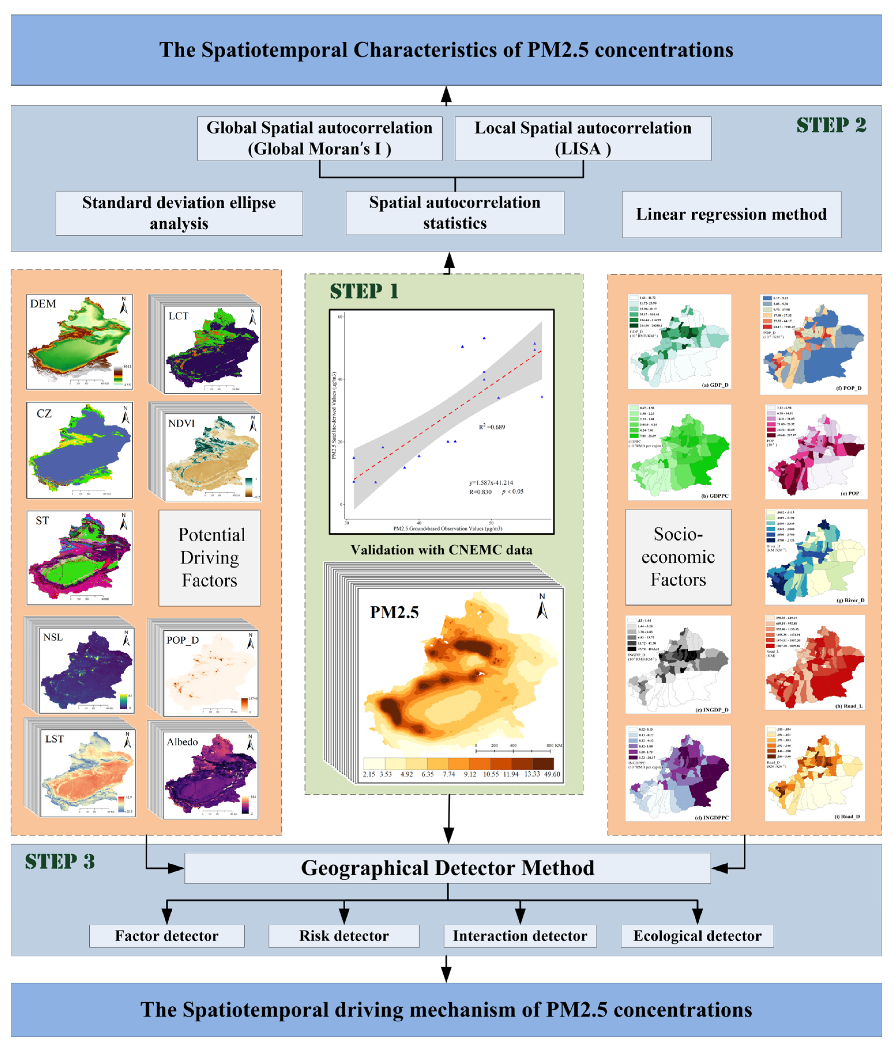
2.3.4. Technical Flowchart of This Study
3. Results
3.1. The Spatio-Temporal Characteristics of PM2.5 Concentrations
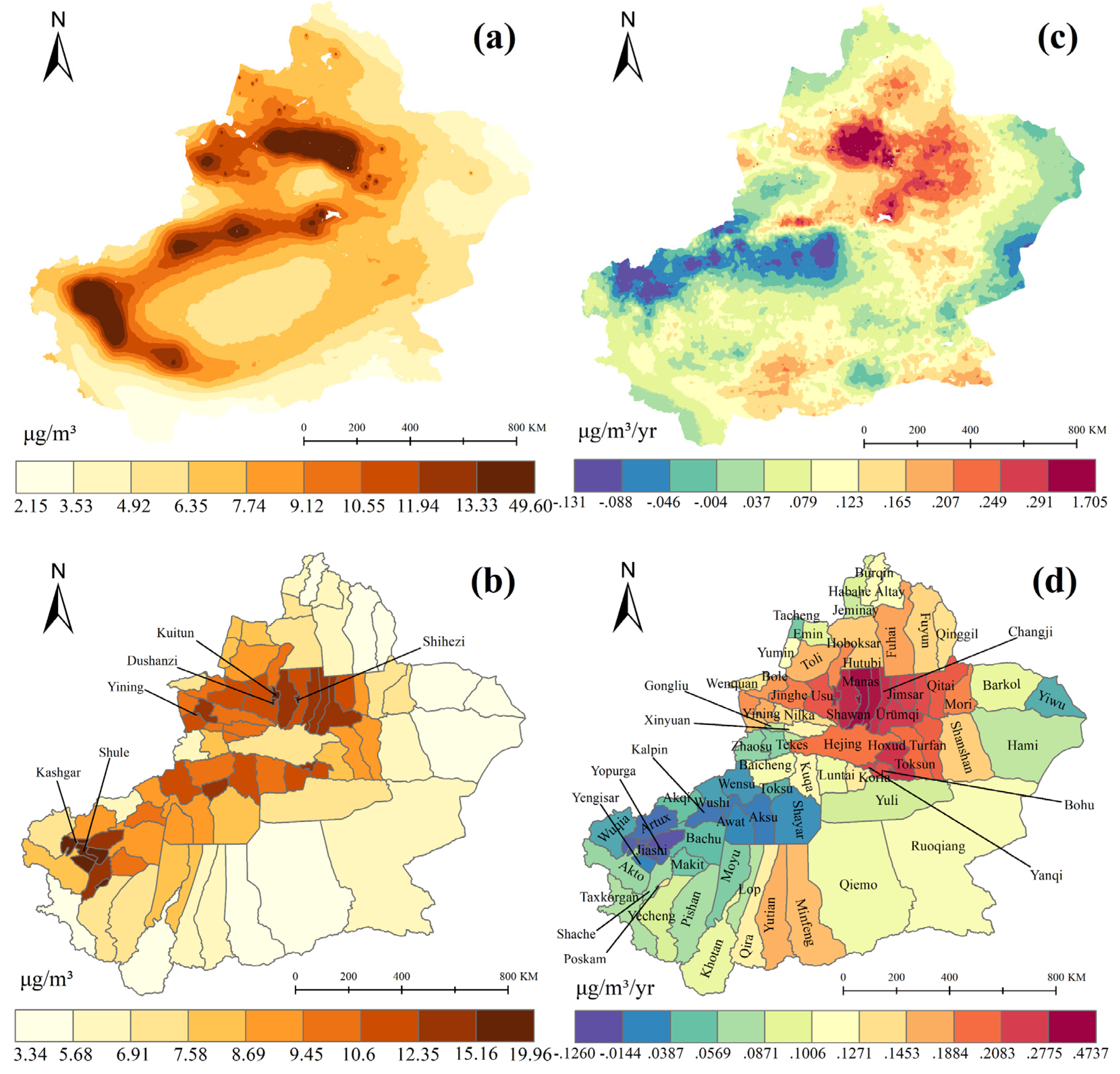
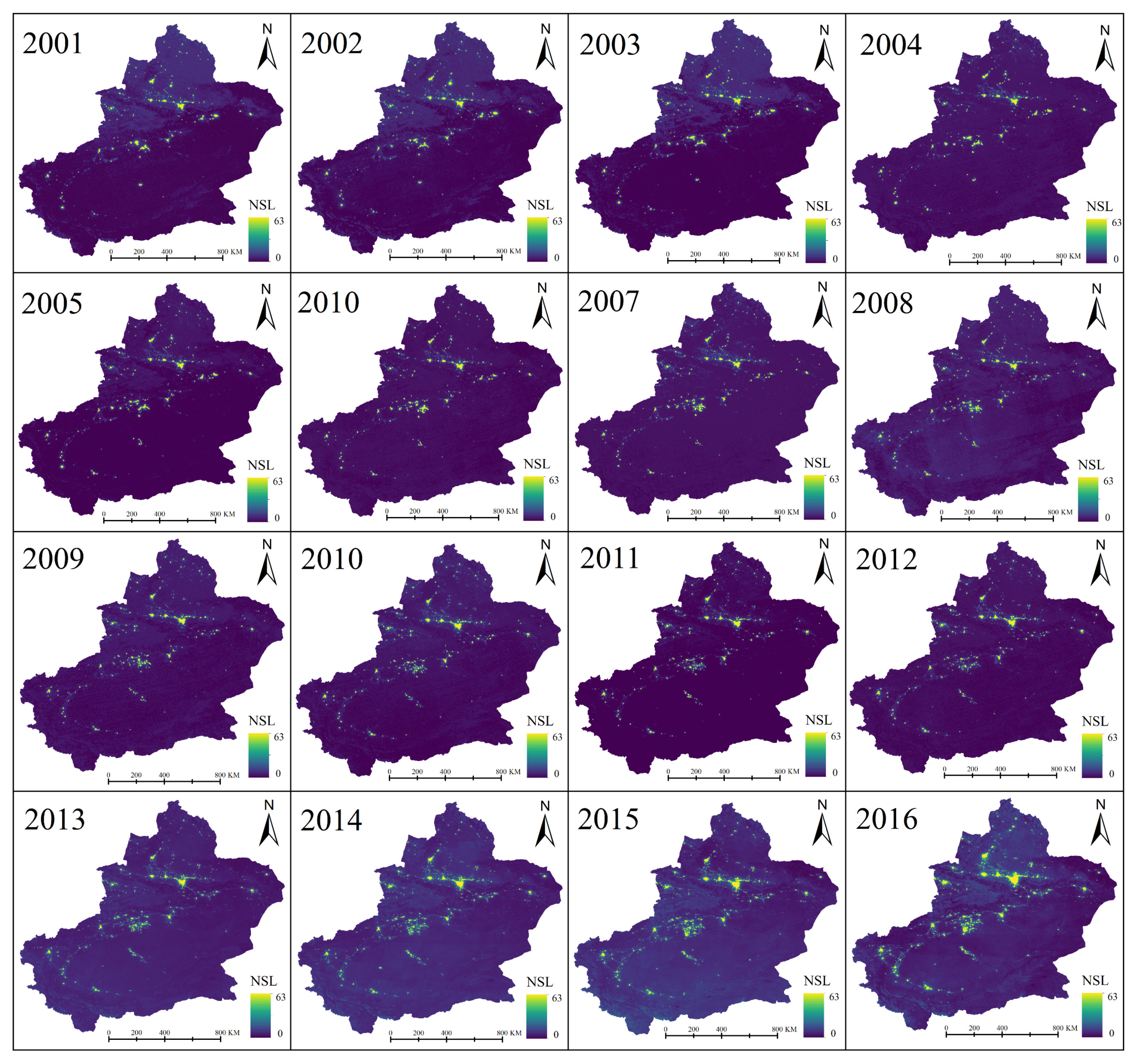
3.1.1. The Spatio-Temporal Pattern and Variation of PM2.5 Concentrations
3.1.2. The Spatial Agglomeration Law of PM2.5 Concentrations
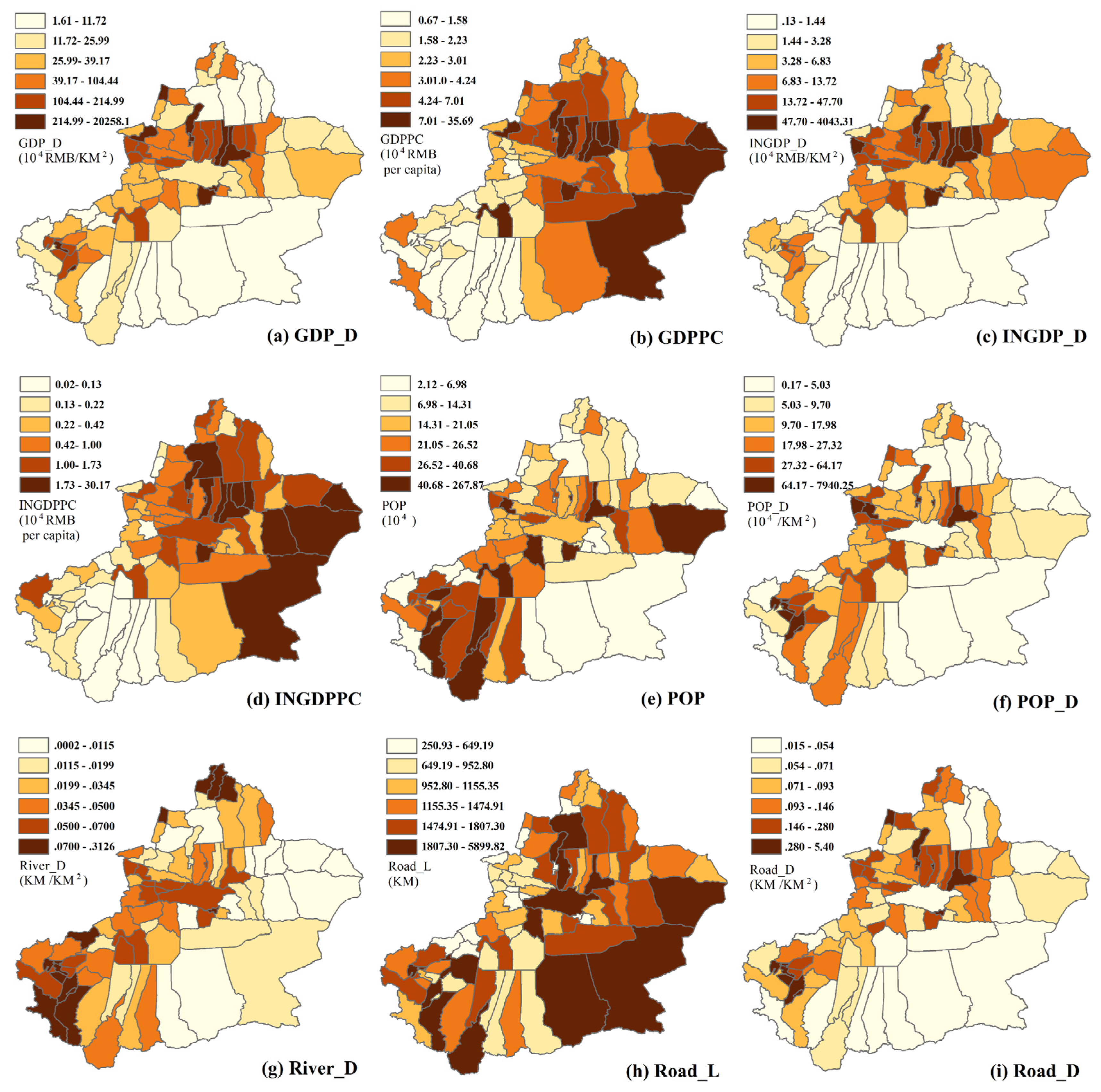
3.2. The Effect of Socio-Economic Factors on PM2.5 Concentations
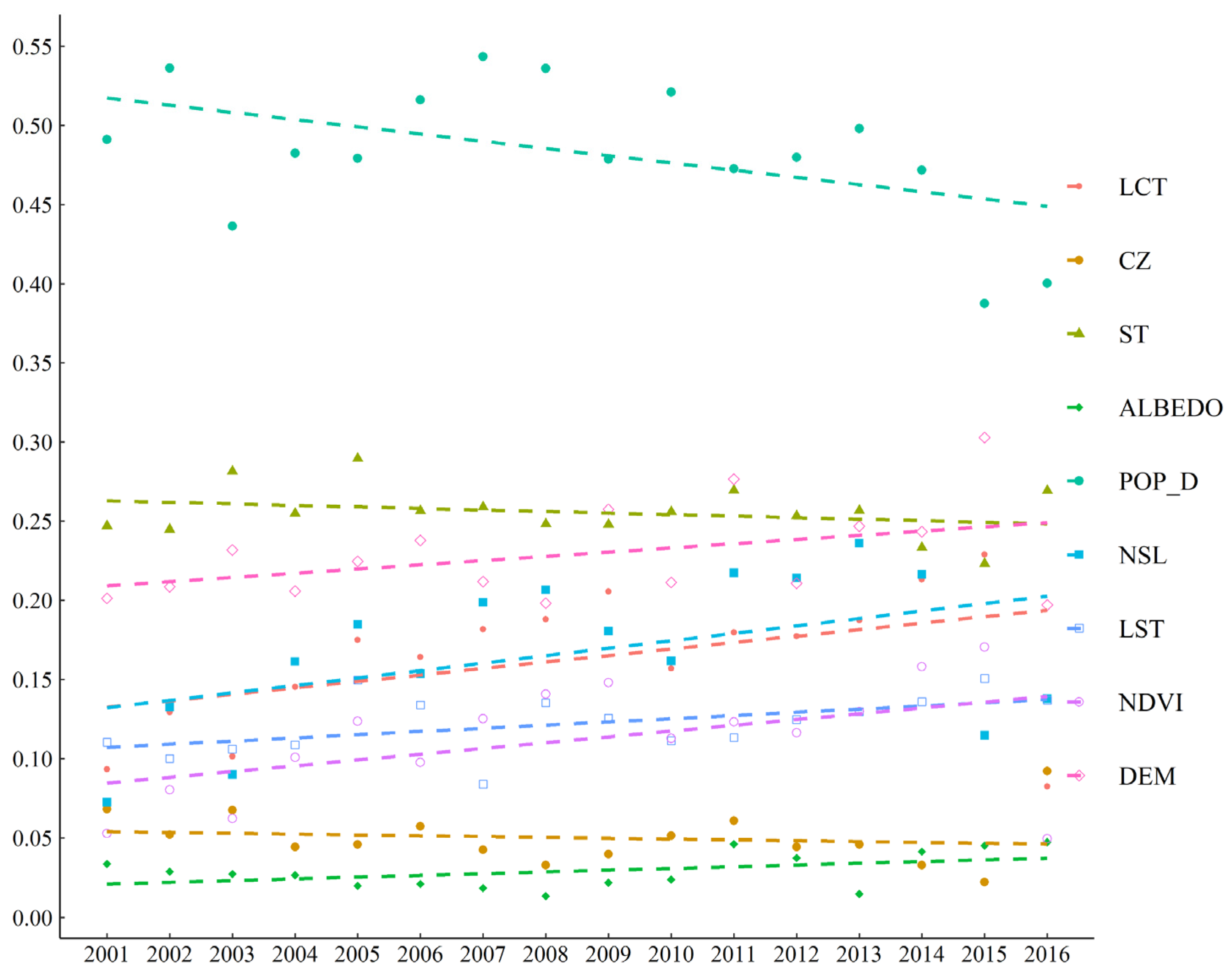
3.3. Interannual Variation of Potential Driving Factors for PM2.5 Concentrations
4. Discussion
5. Conclusions
Author Contributions
Funding
Acknowledgments
Conflicts of Interest
References
- Quarato, M.; De Maria, L.; Gatti, F.M.; Caputi, A.; Mansi, F.; Lorusso, P.; Birtolo, F.; Vimercati, L. Air Pollution and Public Health: A PRISMA-Compliant Systematic Review. Atmosphere 2017, 8, 183. [Google Scholar] [CrossRef] [Green Version]
- Li, Y.G.; Gao, X. Epidemiologic studies of particulate matter and lung cancer. Chin. J. Cancer 2014, 33, 376–380. [Google Scholar] [CrossRef] [Green Version]
- Luo, G.; Zhang, L.; Hu, X.; Qiu, R. Quantifying public health benefits of PM2.5 reduction and spatial distribution analysis in China. Sci. Total Environ. 2020, 719, 137445. [Google Scholar] [CrossRef]
- WHO. World Health Statistics 2016: Monitoring Health for the SDGs Sustainable Development Goals; World Health Organization: Geneva, Switzerland, 2016. [Google Scholar]
- Van, D.A.; Martin, R.V.; Brauer, M.; Hsu, N.C.; Kahn, R.A.; Levy, R.C.; Lyapustin, A.; Sayer, A.M.; Winker, D.M. Global Estimates of Fine Particulate Matter using a Combined Geophysical-Statistical Method with Information from Satellites, Models, and Monitors. Environ. Sci. Technol. 2016, 50, 3762. [Google Scholar]
- Pun, V.C.; Kazemiparkouhi, F.; Manjourides, J.; Suh, H.H. Long-Term PM2.5 Exposure and Respiratory, Cancer, and Cardiovascular Mortality in Older US Adults. Am. J. Epidemiol. 2017, 186, 961–969. [Google Scholar] [CrossRef] [PubMed]
- Hoek, G.; Krishnan, R.M.; Beelen, R.; Peters, A.; Ostro, B.; Brunekreef, B.; Kaufman, J.D. Long-term air pollution exposure and cardio- respiratory mortality: A review. Environ. Health 2013, 12, 43. [Google Scholar] [CrossRef] [PubMed] [Green Version]
- Ramgolam, K.; Favez, O.; Cachier, H.; Gaudichet, A.; Marano, F.; Martinon, L.; Baeza-Squiban, A. Size-partitioning of an urban aerosol to identify particle determinants involved in the proinflammatory response induced in airway epithelial cells. Part. Fibre Toxicol. 2009, 6, 10. [Google Scholar] [CrossRef] [PubMed] [Green Version]
- Zeng, Q.; Shen, L.; Yang, J. Potential impacts of mining of super-thick coal seam on the local environment in arid Eastern Junggar coalfield, Xinjiang region, China. Environ. Earth Sci. 2020, 79, 88. [Google Scholar] [CrossRef]
- Cohen, A.J.; Brauer, M.; Burnett, R.; Anderson, H.R.; Frostad, J.; Estep, K.; Balakrishnan, K.; Brunekreef, B.; Dandona, L.; Dandona, R.; et al. Estimates and 25-year trends of the global burden of disease attributable to ambient air pollution: An analysis of data from the Global Burden of Diseases Study 2015. Lancet 2017, 389, 1907–1918. [Google Scholar] [CrossRef] [Green Version]
- Chen, Z.; Chen, D.; Xie, X.; Cai, J.; Zhuang, Y.; Cheng, N.; He, B.; Gao, B. Spatial self-aggregation effects and national division of city-level PM2.5 concentrations in China based on spatio-temporal clustering. J. Clean. Prod. 2019, 207, 875–881. [Google Scholar] [CrossRef]
- Sun, X.; Luo, X.-S.; Xu, J.; Zhao, Z.; Chen, Y.; Wu, L.; Chen, Q.; Zhang, D. Spatio-temporal variations and factors of a provincial PM2.5 pollution in eastern China during 2013–2017 by geostatistics. Sci. Rep. 2019, 9, 3613. [Google Scholar] [CrossRef] [Green Version]
- Ji, G.; Tian, L.; Zhao, J.; Yue, Y.; Wang, Z. Detecting spatiotemporal dynamics of PM2.5 emission data in China using DMSP-OLS nighttime stable light data. J. Clean. Prod. 2019, 209, 363–370. [Google Scholar] [CrossRef]
- Han, X.; Liu, Y.; Gao, H.; Ma, J.; Mao, X.; Wang, Y.; Ma, X. Forecasting PM 2.5 induced male lung cancer morbidity in China using satellite retrieved PM 2.5 and spatial analysis. Sci. Total Environ. 2017, 607, 1009–1017. [Google Scholar] [CrossRef]
- Jian, P.; Sha, C.; Lü, H.; Liu, Y.; Wu, J. Spatiotemporal patterns of remotely sensed PM 2.5 concentration in China from 1999 to 2011. Remote Sens. Environ. 2016, 174, 109–121. [Google Scholar]
- Chu, H.-J.; Bilal, M. PM2.5 mapping using integrated geographically temporally weighted regression (GTWR) and random sample consensus (RANSAC) models. Environ. Sci. Pollut. Res. 2019, 26, 1902–1910. [Google Scholar] [CrossRef]
- Zhang, Y.; Li, Z. Remote sensing of atmospheric fine particulate matter (PM2.5) mass concentration near the ground from satellite observation. Remote Sens. Environ. 2015, 160, 252–262. [Google Scholar] [CrossRef]
- Luo, J.; Du, P.; Samat, A.; Xia, J.; Che, M.; Xue, Z. Spatiotemporal Pattern of PM2.5 Concentrations in Mainland China and Analysis of Its Influencing Factors using Geographically Weighted Regression. Sci. Rep. 2017, 7, 40607. [Google Scholar] [CrossRef] [PubMed]
- Ma, L.; Gao, Y.; Fu, T.; Cheng, L.; Chen, Z.; Li, M. Estimation of Ground PM2.5 Concentrations using a DEM-assisted Information Diffusion Algorithm: A Case Study in China. Sci. Rep. 2017, 7, 15556. [Google Scholar] [CrossRef] [Green Version]
- Wei, Q.; Zhang, L.; Duan, W.; Zhen, Z. Global and Geographically and Temporally Weighted Regression Models for Modeling PM2.5 in Heilongjiang, China from 2015 to 2018. Int. J. Environ. Res. Public Health 2019, 16, 5107. [Google Scholar] [CrossRef] [PubMed] [Green Version]
- Lu, D.; Xu, J.; Yang, D.; Zhao, J. Spatio-temporal variation and influence factors of PM2.5 concentrations in China from 1998 to 2014. Atmos. Pollut. Res. 2017, 8, 1151–1159. [Google Scholar] [CrossRef]
- Xu, G.; Ren, X.; Xiong, K.; Li, L.; Bi, X.; Wu, Q. Analysis of the driving factors of PM2.5 concentration in the air: A case study of the Yangtze River Delta, China. Ecol. Indic. 2020, 110, 105889. [Google Scholar] [CrossRef]
- Wang, J.F.; Li, X.H.; Christakos, G.; Liao, Y.L.; Zhang, T.; Gu, X.; Zheng, X.Y. Geographical Detectors-Based Health Risk Assessment and its Application in the Neural Tube Defects Study of the Heshun Region, China. Int. J. Geogr. Inf. Sci. 2010, 24, 107–127. [Google Scholar] [CrossRef]
- Shrestha, A.; Luo, W. An assessment of groundwater contamination in Central Valley aquifer, California using geodetector method. Ann. GIS 2017, 23, 149–166. [Google Scholar] [CrossRef]
- Xu, C. Spatio-Temporal Pattern and Risk Factor Analysis of Hand, Foot and Mouth Disease Associated with Under-Five Morbidity in the Beijing–Tianjin–Hebei Region of China. Int. J. Environ. Res. Public Health 2017, 14, 416. [Google Scholar] [CrossRef] [PubMed] [Green Version]
- Yang, T.; Sun, F.; Liu, W.; Wang, H.; Wang, T.; Liu, C. Using Geo-detector to attribute spatio-temporal variation of pan evaporation across China in 1961–2001. Int. J. Climatol. 2019, 39, 2833–2840. [Google Scholar] [CrossRef]
- Zhu, W.; Luo, L.; Cheng, Z.; Yan, N.; Lou, S.; Ma, Y. Characteristics and contributions of biogenic secondary organic aerosol tracers to PM2.5 in Shanghai, China. Atmos. Pollut. Res. 2018, 9, 179–188. [Google Scholar] [CrossRef]
- Ping, S.; Xin, J.; An, J.; Kong, L.; Wang, B.; Wang, J.; Wang, Y.; Dan, W. The empirical relationship between PM 2.5 and AOD in Nanjing of the Yangtze River Delta. Atmos. Pollut. Res. 2016, 8, 233–243. [Google Scholar]
- Li, X.; Zhang, Q.; Zhang, Y.; Zheng, B.; Wang, K.; Chen, Y.; Wallington, T.J.; Han, W.; Shen, W.; Zhang, X. Source contributions of urban PM 2.5 in the Beijing–Tianjin–Hebei region: Changes between 2006 and 2013 and relative impacts of emissions and meteorology. Atmos. Environ. 2015, 123, 229–239. [Google Scholar] [CrossRef] [Green Version]
- Turap, Y.; Talifu, D.; Wang, X.; Abulizi, A.; Maihemuti, M.; Tursun, Y.; Ding, X.; Aierken, T.; Rekefu, S. Temporal distribution and source apportionment of PM2.5 chemical composition in Xinjiang, NW-China. Atmos. Res. 2019, 218, 257–268. [Google Scholar] [CrossRef]
- Zhou, C.; Zhao, C.X.; Yang, Z.P. Strategies for environmentally friendly development in the Northern Tianshan Mountain Economic Zone based on scenario analysis. J. Clean. Prod. 2017, 156, 74–82. [Google Scholar] [CrossRef]
- Chen, J.; Lu, J.; Ning, J.; Yan, Y.; Li, S.; Zhou, L. Pollution characteristics, sources, and risk assessment of heavy metals and perfluorinated compounds in PM2.5 in the major industrial city of northern Xinjiang, China. Air Qual. Atmos. Health 2019, 12, 909–918. [Google Scholar] [CrossRef]
- Turap, Y.; Talifu, D.; Wang, X.; Aierken, T.; Rekefu, S.; Shen, H.; Ding, X.; Maihemuti, M.; Tursun, Y.; Liu, W. Concentration characteristics, source apportionment, and oxidative damage of PM2.5-bound PAHs in petrochemical region in Xinjiang, NW China. Environ. Sci. Pollut. Res. 2018, 25, 22629–22640. [Google Scholar] [CrossRef] [PubMed]
- Liu, Y.Y.; Shen, Y.X.; Liu, C.; Liu, H.F. Enrichment and assessment of the health risks posed by heavy metals in PM1 in Changji, Xinjiang, China. J. Environ. Sci. Health Part A 2017, 52, 413–419. [Google Scholar] [CrossRef] [PubMed]
- Li, W.; Ali, E.; Abou El-Magd, I.; Mourad, M.M.; El-Askary, H. Studying the Impact on Urban Health over the Greater Delta Region in Egypt Due to Aerosol Variability Using Optical Characteristics from Satellite Observations and Ground-Based AERONET Measurements. Remote Sens. 2019, 11, 1998. [Google Scholar] [CrossRef] [Green Version]
- Sorek-Hamer, M.; Kloog, I.; Koutrakis, P.; Strawa, A.W.; Chatfield, R.; Cohen, A.; Ridgway, W.L.; Broday, D.M. Assessment of PM2.5 concentrations over bright surfaces using MODIS satellite observations. Remote Sens. Environ. 2015, 163, 180–185. [Google Scholar] [CrossRef]
- Kloog, I.; Sorek-Hamer, M.; Lyapustin, A.; Coull, B.; Wang, Y.; Just, A.C.; Schwartz, J.; Broday, D.M. Estimating daily PM2.5 and PM10 across the complex geo-climate region of Israel using MAIAC satellite-based AOD data. Atmos. Environ. 2015, 122, 409–416. [Google Scholar] [CrossRef] [Green Version]
- Aina, A.Y.; Van der Merwe, H.J.; Alshuwaikhat, M.H. Spatial and Temporal Variations of Satellite-Derived Multi-Year Particulate Data of Saudi Arabia: An Exploratory Analysis. Int. J. Environ. Res. Public Health 2014, 11. [Google Scholar] [CrossRef] [Green Version]
- Munir, S.; Gabr, S.; Habeebullah, T.M.; Janajrah, M.A. Spatiotemporal analysis of fine particulate matter (PM2.5) in Saudi Arabia using remote sensing data. Egypt. J. Remote Sens. Space Sci. 2016, 19, 195–205. [Google Scholar] [CrossRef]
- Jia, B.; Zhang, Z.; Ci, L.; Ren, Y.; Pan, B.; Zhang, Z. Oasis land-use dynamics and its influence on the oasis environment in Xinjiang, China. J. Arid Environ. 2004, 56, 11–26. [Google Scholar] [CrossRef]
- National Bureau of Statistics of China. China Statistical Yearbook-2019; China Statistics Press: Beijing, China, 2019.
- Liu, Y.; Li, L.; Chen, X.; Zhang, R.; Yang, J. Temporal-spatial variations and influencing factors of vegetation cover in Xinjiang from 1982 to 2013 based on GIMMS-NDVI3g. Glob. Planet. Chang. 2018, 169, 145–155. [Google Scholar] [CrossRef]
- Yang, D.; Ye, C.; Wang, X.; Lu, D.; Xu, J.; Yang, H. Global distribution and evolvement of urbanization and PM2.5 (1998–2015). Atmos. Environ. 2018, 182, 171–178. [Google Scholar] [CrossRef]
- Friedl, M.; Sulla-Menashe, D. MCD12Q1 MODIS/Terra+ Aqua land cover type yearly L3 global 500m SIN grid V006 NASA EOSDIS Land Processes DAAC: 2015.
- Wan, Z.; Hook, S.; Hulley, G. MOD11A2 MODIS/Terra land surface temperature/emissivity 8-day L3 global 1km SIN grid V006. NASA EOSDIS Land Processes DAAC: 2015.
- Didan, K. MOD13Q1 MODIS/Terra vegetation indices 16-day L3 global 250m SIN grid V006. NASA EOSDIS Land Processes DAAC: 2015.
- Schaaf, C.; Wang, Z. MCD43A3 MODIS/Terra+ Aqua BRDF/Albedo Daily L3 Global—500 m V006. NASA EOSDIS Land Processes DAAC: 2015.
- Román, M.O.; Schaaf, C.B.; Lewis, P.; Gao, F.; Anderson, G.P.; Privette, J.L.; Strahler, A.H.; Woodcock, C.E.; Barnsley, M. Assessing the coupling between surface albedo derived from MODIS and the fraction of diffuse skylight over spatially-characterized landscapes. Remote Sens. Environ. 2010, 114, 738–760. [Google Scholar] [CrossRef]
- Small, C.; Elvidge, C.D. Night on Earth: Mapping decadal changes of anthropogenic night light in Asia. Int. J. Appl. Earth Obs. Geoinf. 2013, 22, 40–52. [Google Scholar] [CrossRef] [Green Version]
- Bennett, M.M.; Smith, L.C. Advances in using multitemporal night-time lights satellite imagery to detect, estimate, and monitor socioeconomic dynamics. Remote Sens. Environ. 2017, 192, 176–197. [Google Scholar] [CrossRef]
- Forbes, D.J. Multi-scale analysis of the relationship between economic statistics and DMSP-OLS night light images. GIScience Remote Sens. 2013, 50, 483–499. [Google Scholar] [CrossRef]
- Reuter, H.I.; Nelson, A.; Jarvis, A. An evaluation of void-filling interpolation methods for SRTM data. Int. J. Geogr. Inf. Sci. 2007, 21, 983–1008. [Google Scholar] [CrossRef]
- Beck, H.E.; Zimmermann, N.E.; McVicar, T.R.; Vergopolan, N.; Berg, A.; Wood, E.F. Present and future Köppen-Geiger climate classification maps at 1-km resolution. Sci. Data 2018, 5, 180214. [Google Scholar] [CrossRef] [Green Version]
- Tatem, A.J. WorldPop, open data for spatial demography. Sci. Data 2017, 4, 1–4. [Google Scholar] [CrossRef] [PubMed]
- Lefever, D.W. Measuring Geographic Concentration by Means of the Standard Deviational Ellipse. Am. J. Sociol. 1926, 32, 88–94. [Google Scholar] [CrossRef]
- Moran, P.A.P. Notes on Continuous Stochastic Phenomena. Biometrika 1950, 37, 17–23. [Google Scholar] [CrossRef]
- Anselin, L. Local Indicators of Spatial Association—LISA. Geogr. Anal. 1995, 27, 93–115. [Google Scholar] [CrossRef]
- Welcome to Visit the GeoDetector Website. Available online: www.geodetector.cn (accessed on 19 March 2019).
- Wang, B.; Lai, X. Report on the Development of Emerging Special Economic Zones in Xinjiang. In Annual Report on the Development of China’s Special Economic Zones(2018): Blue Book of China’s Special Economic Zones; Tao, Y., Yuan, Y., Eds.; Springer: Singapore, 2019; pp. 75–92. [Google Scholar] [CrossRef]
- Han, X.; Li, G. The Development Trend and Prediction Model of Xinjiang GDP in the Context of “One Belt and One Road”. In Proceedings of the 2018 10th International Conference on Measuring Technology and Mechatronics Automation (ICMTMA), Changsha, China, 10–11 February 2018; pp. 468–471. [Google Scholar]
- Xu, J.; Yu, D.; Fan, B.; Zeng, X.; Lv, W.; Chen, J. Characterization of Ash Particles from Co-combustion with a Zhundong Coal for Understanding Ash Deposition Behavior. Energy Fuels 2014, 28, 678–684. [Google Scholar] [CrossRef]
- Qiu, X.; Duan, L.; Gao, J.; Wang, S.; Chai, F.; Hu, J.; Zhang, J.; Yun, Y. Chemical composition and source apportionment of PM10 and PM2.5 in different functional areas of Lanzhou, China. J. Environ. Sci. 2016, 40, 75–83. [Google Scholar] [CrossRef]
- Guo, W.; Xia, N.; Tashpolat, T.; Wang, J.; Nigara, T.; Yang, C. Inversion of PM2. 5 and PM10 content based on AOD data in large opencast coal mining area of Xinjiang. Trans. Chin. Soc. Agric. Eng. 2017, 33, 216–222. [Google Scholar]
- Lin, G.; Fu, J.; Jiang, D.; Hu, W.; Dong, D.; Huang, Y.; Zhao, M. Spatio-Temporal Variation of PM2.5 Concentrations and Their Relationship with Geographic and Socioeconomic Factors in China. Int. J. Environ. Res. Public Health 2014, 11. [Google Scholar] [CrossRef] [PubMed] [Green Version]
- Wang, S.; Zhou, C.; Wang, Z.; Feng, K.; Hubacek, K. The characteristics and drivers of fine particulate matter (PM2.5) distribution in China. J. Clean. Prod. 2017, 142, 1800–1809. [Google Scholar] [CrossRef]
- Han, L.; Zhou, W.; Li, W.; Li, L. Impact of urbanization level on urban air quality: A case of fine particles (PM2.5) in Chinese cities. Environ. Pollut. 2014, 194, 163–170. [Google Scholar] [CrossRef]
- Liu, Y.; Cao, G.; Zhao, N.; Mulligan, K.; Ye, X. Improve ground-level PM2.5 concentration mapping using a random forests-based geostatistical approach. Environ. Pollut. 2018, 235, 272–282. [Google Scholar] [CrossRef]
- National Bureau of Statistics of China. China Statistical Yearbook-2001; China Statistics Press: Beijing, China, 2001.
- Xu, J.; Chen, Y.; Li, W.; Liu, Z.; Tang, J.; Wei, C. Understanding temporal and spatial complexity of precipitation distribution in Xinjiang, China. Theor. Appl. Climatol. 2016, 123, 321–333. [Google Scholar] [CrossRef]
- Mamat, T.; Ding, W.; Kasim, E.; Hassan, M. The sustainable development of agricultural mechanization based on combination weighting and ahp. Chin. J. Agric. Resour. Reg. Plan. 2018, 39, 67–73. [Google Scholar]
- Liu, Q.; Yang, Z.; Wang, C.; Han, F. Temporal-Spatial Variations and Influencing Factor of Land Use Change in Xinjiang, Central Asia, from 1995 to 2015. Sustainability 2019, 11, 696. [Google Scholar] [CrossRef] [Green Version]
- Liu, S.S.; Zhang, Q.; Li, X.C.; Song, W.J.; Yang, J.N.; Liu, X.J. Temporal and Spatial Variations of Vegetation Cover in Xinjiang from 2002 to 2015 and Their Response to Climate. IOP Conf. Ser. Earth Environ. Sci. 2017, 74, 012021. [Google Scholar] [CrossRef] [Green Version]


| Dataset | Data Sources | Spatial Resolution | Temporal Resolution |
|---|---|---|---|
| LCT | MODIS MCD12Q1 (2001–2016) | 500 m | 1 year |
| LST | MODIS MOD11A2 (2001–2016) | 1000 m | 8 day |
| NDVI | MODIS MOD13Q1 (2001–2016) | 250 m | 16 day |
| Albedo | MODIS MCD43A3 (2001–2016) | 500 m | 1 day |
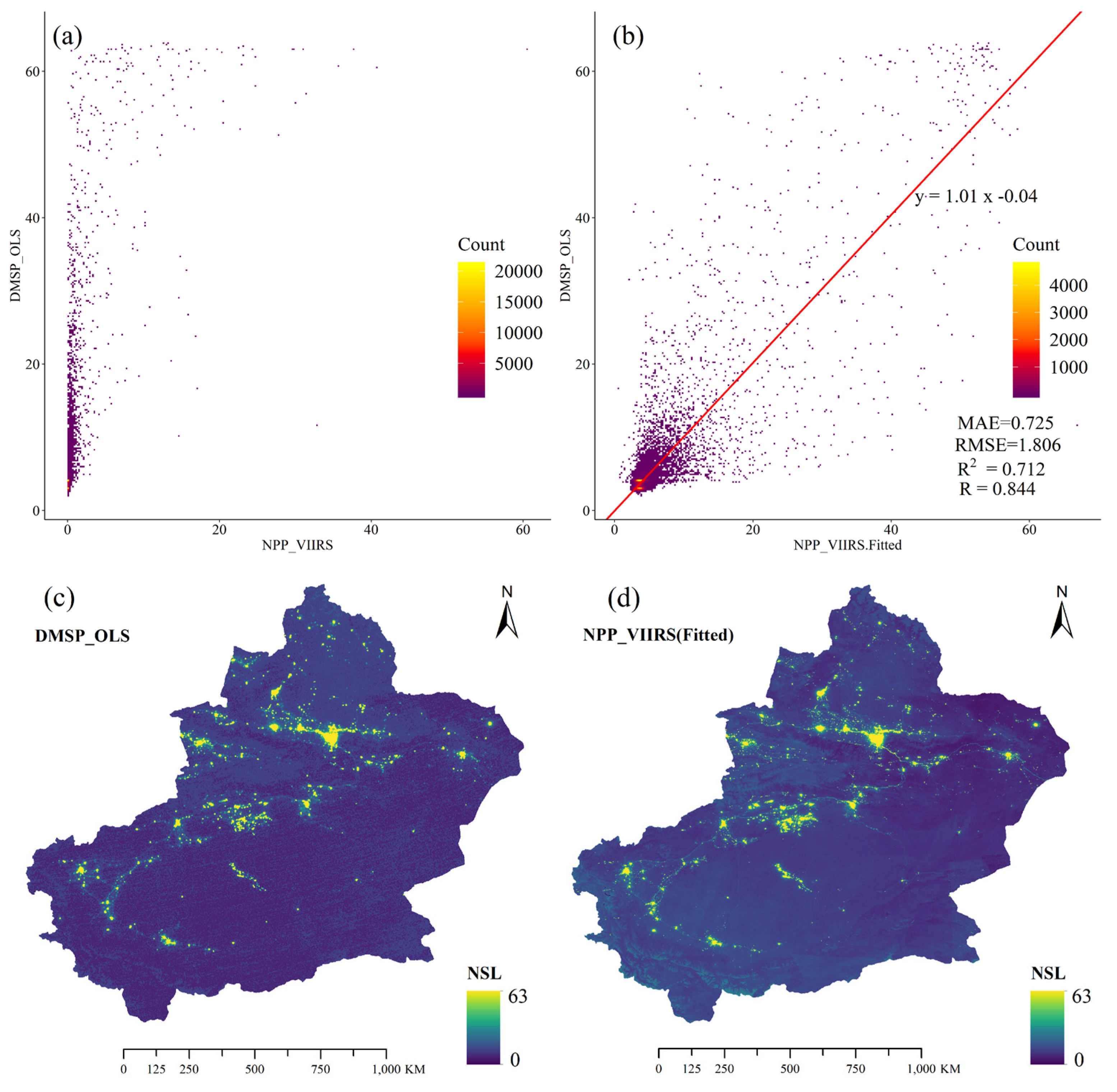
| NSL | DMSP-OLS (2001–2013) /NPP-VIIRS (2013–2016) | 1000 m/500 m | 1 year/ 1 month |
| DEM | NASA Shuttle Radar Topographic Mission | 90 m | - |
| CZ | Köppen-Geiger climate classification maps (2000–2015) | 1 km | - |
| POP | Asia Continental Population Dataset (2000–2015) and 2017 Xinjiang Statistical Year book | 1 km | 5 year |
| GDP | 2017 Xinjiang Statistical Year book | - | - |
| INGDP | 2017 Xinjiang Statistical Year book | - | - |
| Road_L | OpenStreetMap historical dataset | - | - |
| River_L | OpenStreetMap historical dataset | - | - |
| Acronyms | Full Name | Acronyms | Full Name |
|---|---|---|---|
| ACAG | Atmospheric Composition Analysis Group | LST | Land surface temperature |
| AERONET | Aerosol Robotic Network | MAE | Mean Absolute Error |
| AOD | Aerosol Optical Depth | MAIAC | Multi-angle implementation of atmospheric correction |
| BSA | Black-sky albedo | MISR | Multiangle Imaging Spectroradiometer |
| CNEMC | Chinese National Environmental Monitoring Center | LISA | Local Indicators of Spatial Association |
| CRU | Climatic Research Unit | MODIS | Moderate Resolution Imaging Spectroradiometer |
| CZ | Climate Zone | NASA-SRTM | National Aeronautics and Space Administration Shuttle Radar Topographic Mission |
| DB | Deep Blue | NDVI | Normalized Difference Vegetation Index |
| DEM | Digital elevation model | NGDC | National Geophysical Data Center |
| DMSP-OLS | Defense Meteorological Satellite Program’s Operational Line-Scan System | NPP-VIIRS | Suomi National Polar-Orbiting Partnership Visible Infrared Imaging Radiometer Suite |
| DT | Dark Target | NSL | Nighttime stable light |
| GBD | Global Burden of Disease | NTMEZ | North Tianshan Mountain Economic Zone |
| GDM | Geographical detector method | OSM | OpenStreetMap |
| GDP | Gross Domestic Product | PFCs | Per fluorinated compounds |
| GDP_D | GDP density | PM2.5 | Particulate matter with a diameter of 2.5 μm or less |
| GDPPC | GDP per capita | POP | Population |
| GIMMS | Global Inventory Modelling and Mapping Studies | POP_D | POP density |
| GPCC | Global Precipitation Climatology Center | RMSE | Root Mean Square Error |
| GTWR | Geographically and Temporally Weighted Regression | Road_L | Road length |
| GWR | Geographically Weighted Regression | Road_D | Road density |
| HMs | Heavy metals | River_L | River length |
| IGBP | International Geosphere-Biosphere Programme | River_D | River density |
| INGDP | Industrial GDP | SDE | Standard deviational ellipse |
| INGDP_D | INGDP density | SeaWiFS | Sea-Viewing Wide Field-of-View Sensor |
| INGDPPC | INGDP per capita | WHO | World Health Organization |
| LCT | Land cover type | WSA | White-sky albedo |
| Local Moran’s I | p Value | ZI-Score | Spatial Autocorrelation Types |
|---|---|---|---|
| Positive | p > 0.05 | ZI > 0 | High-High Cluster |
| Positive | p > 0.05 | ZI < 0 | Low-Low Cluster |
| Negative | p > 0.05 | ZI > 0 | High-Low Outlier |
| Negative | p > 0.05 | ZI < 0 | Low-High Outlier |
| Interaction Type | Description |
|---|---|
| Weaken, univariate | Min(q(X1), q(X2)) < q(X1∩X2) < Max(q(X1)), q(X2)) |
| Weaken, non-linear | q(X1∩X2) < Min(q(X1), q(X2)) |
| Enhance, bivariate | q(X1∩X2)> Max(q(X1), q(X2)) |
| Enhance, non-linear | q(X1∩X2) > q(X1) + q(X2) |
| Independent | q(X1∩X2) = q(X1) + q(X2) |
© 2020 by the authors. Licensee MDPI, Basel, Switzerland. This article is an open access article distributed under the terms and conditions of the Creative Commons Attribution (CC BY) license (http://creativecommons.org/licenses/by/4.0/).
Share and Cite
Wang, W.; Samat, A.; Abuduwaili, J.; Ge, Y. Spatio-Temporal Variations of Satellite-Based PM2.5 Concentrations and Its Determinants in Xinjiang, Northwest of China. Int. J. Environ. Res. Public Health 2020, 17, 2157. https://0-doi-org.brum.beds.ac.uk/10.3390/ijerph17062157
Wang W, Samat A, Abuduwaili J, Ge Y. Spatio-Temporal Variations of Satellite-Based PM2.5 Concentrations and Its Determinants in Xinjiang, Northwest of China. International Journal of Environmental Research and Public Health. 2020; 17(6):2157. https://0-doi-org.brum.beds.ac.uk/10.3390/ijerph17062157
Chicago/Turabian StyleWang, Wei, Alim Samat, Jilili Abuduwaili, and Yongxiao Ge. 2020. "Spatio-Temporal Variations of Satellite-Based PM2.5 Concentrations and Its Determinants in Xinjiang, Northwest of China" International Journal of Environmental Research and Public Health 17, no. 6: 2157. https://0-doi-org.brum.beds.ac.uk/10.3390/ijerph17062157