
Comparison of ARIMA and LSTM in Forecasting the Incidence of HFMD Combined and Uncombined with Exogenous Meteorological Variables in Ningbo, China

 , ,
, ,
Abstract
:1. Introduction
2. Materials and Methods
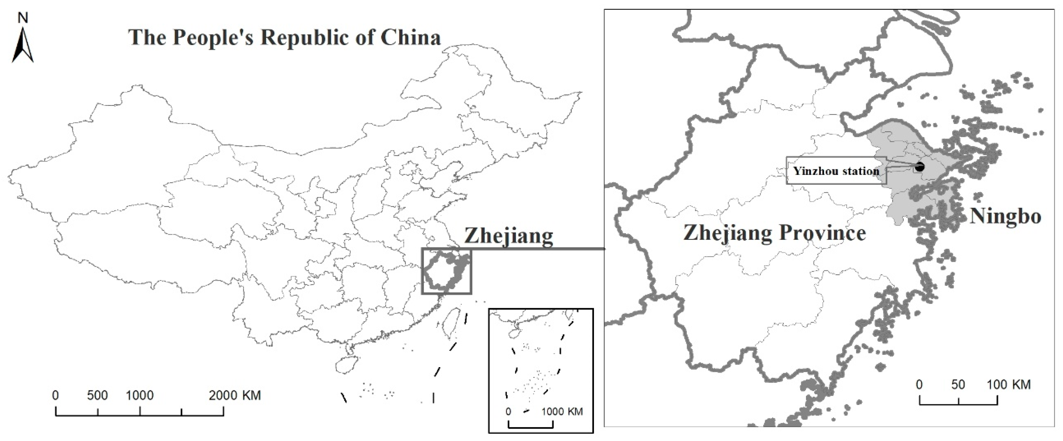
2.1. Study Area
2.2. HFMD Incidence and Meteorological Data
2.3. Data Analysis
2.3.1. ARIMA Model
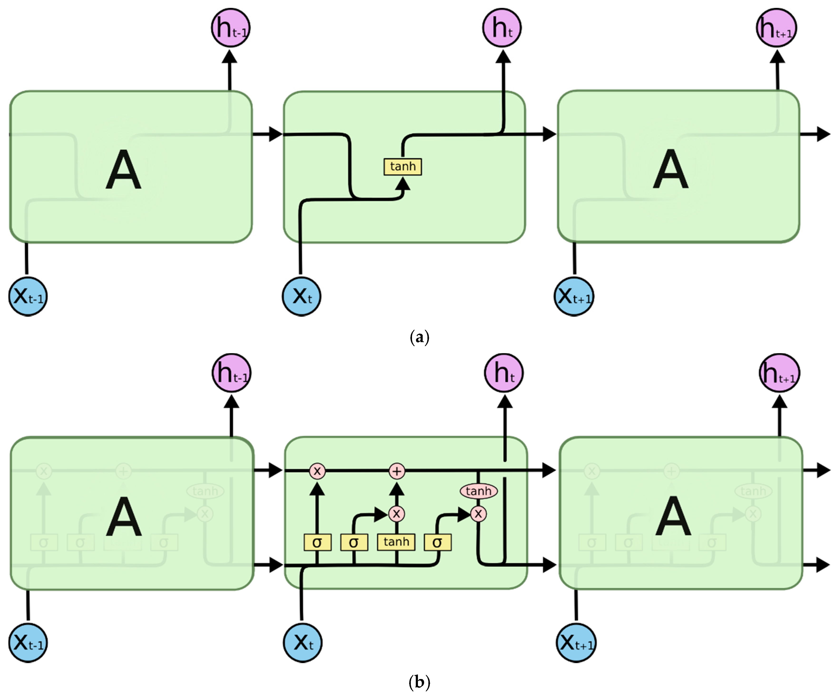
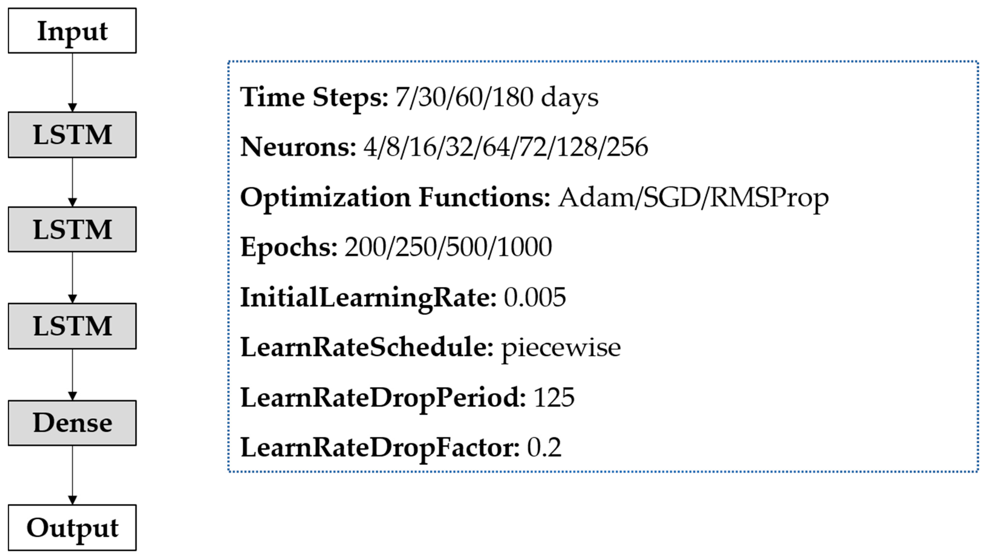
2.3.2. LSTM Model
2.3.3. One Step Ahead Rolling Forecast
3. Results
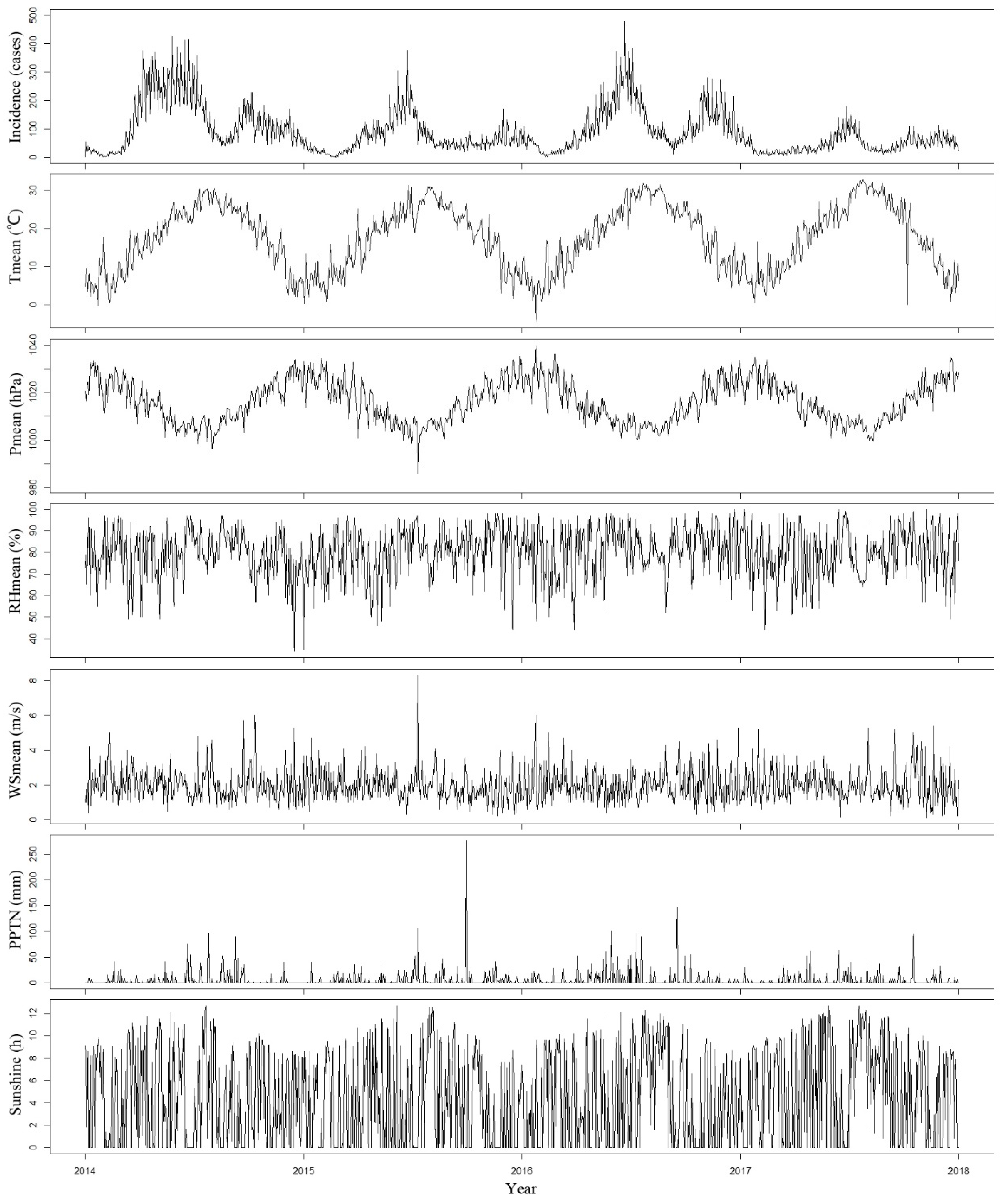
3.1. Descriptive Analysis
3.2. ARIMA and ARIMAX Model
3.3. Univariate LSTM and Multivariable LSTM Model
3.4. Prediction Performance Comparison
4. Discussion
5. Conclusions
Supplementary Materials
Author Contributions
Funding
Institutional Review Board Statement
Informed Consent Statement
Data Availability Statement
Conflicts of Interest
References
- Du, Z.; Zhang, W.; Zhang, D.; Yu, S.; Hao, Y. Estimating the basic reproduction rate of HFMD using the time series SIR model in Guangdong, China. PLoS ONE 2017, 12, e0179623. [Google Scholar] [CrossRef] [Green Version]
- Yu, L.; Zhou, L.; Tan, L.; Jiang, H.; Wang, Y.; Wei, S.; Nie, S. Application of a new hybrid model with seasonal auto-regressive integrated moving average (ARIMA) and nonlinear auto-regressive neural network (NARNN) in forecasting incidence cases of HFMD in Shenzhen, China. PLoS ONE 2014, 9, e98241. [Google Scholar]
- Bo, Y.-C.; Song, C.; Wang, J.-F.; Li, X.-W. Using an autologistic regression model to identify spatial risk factors and spatial risk patterns of hand, foot and mouth disease (HFMD) in Mainland China. BMC Public Health 2014, 14, 358. [Google Scholar] [CrossRef] [PubMed] [Green Version]
- Sumi, A.; Toyoda, S.; Kanou, K.; Fujimoto, T.; Mise, K.; Kohei, Y.; Koyama, A.; Kobayashi, N. Association between meteorological factors and reported cases of hand, foot, and mouth disease from 2000 to 2015 in Japan. Epidemiol. Infect. 2017, 145, 2896–2911. [Google Scholar] [CrossRef] [Green Version]
- Bendig, J.W.; Fleming, D.M. Epidemiological, virological, and clinical features of an epidemic of hand, foot, and mouth disease in England and Wales. Commun. Dis. Rep. CDR Rev. 1996, 6, R81–R86. [Google Scholar]
- Liu, W.; Bao, C.; Zhou, Y.; Ji, H.; Wu, Y.; Shi, Y.; Shen, W.; Bao, J.; Li, J.; Hu, J.; et al. Forecasting incidence of hand, foot and mouth disease using BP neural networks in Jiangsu province, China. BMC Infect. Dis. 2019, 19, 1–9. [Google Scholar] [CrossRef] [PubMed] [Green Version]
- Zhong, R.; Wu, Y.; Cai, Y.; Wang, R.; Zheng, J.; Lin, D.; Wu, H.; Li, Y. Forecasting hand, foot, and mouth disease in Shenzhen based on daily level clinical data and multiple environmental factors. Biosci. Trends 2018, 12, 450–455. [Google Scholar] [CrossRef] [Green Version]
- Liu, L.; Luan, R.S.; Yin, F.; Zhu, X.P.; Lu, Q. Predicting the incidence of hand, foot and mouth disease in Sichuan province, China using the ARIMA model. Epidemiol. Infect. 2016, 144, 144–151. [Google Scholar] [CrossRef] [PubMed] [Green Version]
- Cryer, J.D.; Chan, K.-S. Time Series Analysis with Applications in R; Springer: Berlin/Heidelberg, Germany, 2010. [Google Scholar]
- Yang, Q.; Wang, J.; Ma, H.; Wang, X. Research on COVID-19 based on ARIMA model (Delta)—Taking Hubei, China as an example to see the epidemic in Italy. J. Infect. Public Health 2020, 13, 1415–1418. [Google Scholar] [CrossRef] [PubMed]
- Wang, Y.-W.; Shen, Z.-Z.; Jiang, Y. Comparison of ARIMA and GM(1,1) models for prediction of hepatitis B in China. PLoS ONE 2018, 13, e0201987. [Google Scholar] [CrossRef] [PubMed]
- He, Z.; Tao, H. Epidemiology and ARIMA model of positive-rate of influenza viruses among children in Wuhan, China: A nine-year retrospective study. Int. J. Infect. Dis. 2018, 74, 61–70. [Google Scholar] [CrossRef] [Green Version]
- Wang, K.W.; Deng, C.; Li, J.P.; Zhang, Y.Y.; Li, X.Y.; Wu, M.C. Hybrid methodology for tuberculosis incidence time-series forecasting based on ARIMA and a NAR neural network. Epidemiol. Infect. 2017, 145, 1118–1129. [Google Scholar] [CrossRef] [Green Version]
- Yang, J.; Li, L.; Shi, Y.; Xie, X. An ARIMA Model with Adaptive Orders for Predicting Blood Glucose Concentrations and Hypoglycemia. IEEE J. Biomed. Health Inform. 2018, 23, 1251–1260. [Google Scholar] [CrossRef]
- Luo, L.; Luo, L.; Zhang, X.; He, X. Hospital daily outpatient visits forecasting using a combinatorial model based on ARIMA and SES models. BMC Health Serv. Res. 2017, 17, 469. [Google Scholar] [CrossRef] [PubMed] [Green Version]
- Kim, T.; Kim, H.Y. Forecasting stock prices with a feature fusion LSTM-CNN model using different representations of the same data. PLoS ONE 2019, 14, e0212320. [Google Scholar] [CrossRef] [PubMed]
- Kim, M.; Cao, B.; Mau, T.; Wang, J. Speaker-Independent Silent Speech Recognition from Flesh-Point Articulatory Movements Using an LSTM Neural Network. IEEE/ACM Trans. Audio Speech Lang. Process 2017, 25, 2323–2336. [Google Scholar] [CrossRef]
- Gu, J.; Liang, L.; Song, H.; Kong, Y.; Ma, R.; Hou, Y.; Zhao, J.; Liu, J.; He, N.; Zhang, Y. A method for hand-foot-mouth disease prediction using GeoDetector and LSTM model in Guangxi, China. Sci. Rep. 2019, 9, 1–10. [Google Scholar] [CrossRef]
- Kirbas, I.; Sozen, A.; Tuncer, A.D.; Kazancioglu, F.S. Comparative analysis and forecasting of COVID-19 cases in various European countries with ARIMA, NARNN and LSTM approaches. Chaos Solitons Fractals 2020, 138, 110015. [Google Scholar] [CrossRef]
- Wang, G.; Wei, W.; Jiang, J.; Ning, C.; Chen, H.; Huang, J.; Liang, B.; Zang, N.; Liao, Y.; Chen, R.; et al. Application of a long short-term memory neural network: A burgeoning method of deep learning in forecasting HIV incidence in Guangxi, China. Epidemiol. Infect. 2019, 147, e194. [Google Scholar] [CrossRef] [PubMed] [Green Version]
- Jing, Q.L.; Cheng, Q.; Marshall, J.M.; Hu, W.; Yang, Z.C.; Lu, J.H. Imported cases and minimum temperature drive dengue transmission in Guangzhou, China: Evidence from ARIMAX model. Epidemiol. Infect. 2018, 146, 1226–1235. [Google Scholar] [CrossRef] [Green Version]
- National Population and Health Science Data Sharing Platform: The Datacenter of China Public Health Science. Available online: http://www.phsciencedata.cn/Share/en/index.jsp (accessed on 25 March 2020).
- Paul, J.C.; Hoque, M.S.; Morshedur, R.M. Selection of Best ARIMA Model for Forecasting Average Daily Share Price Index of Pharmaceutical Companies in Bangladesh: A Case Study on Square Pharmaceutical Ltd. Glob. J. Manag. Bus. Res. 2013, 13, 14–25. [Google Scholar]
- Aboagye-Sarfo, P.; Mai, Q.; Sanfilippo, F.M.; Preen, D.B.; Stewart, L.M.; Fatovich, D.M. A comparison of multivariate and univariate time series approaches to modelling and forecasting emergency department demand in Western Australia. J. Biomed. Inform. 2015, 57, 62–73. [Google Scholar] [CrossRef] [Green Version]
- Introduction to ARIMA Models. Available online: https://people.duke.edu/~rnau/411arim.htm (accessed on 2 December 2020).
- Hochreiter, S.; Schmidhuber, J. Long Short-Term Memory. Neural. Comput. 1997, 9, 1735–1780. [Google Scholar] [CrossRef]
- Understanding LSTM Networks. Available online: https://colah.github.io/posts/2015-08-Understanding-LSTMs/ (accessed on 15 January 2021).
- Chae, S.; Kwon, S.; Lee, D. Predicting Infectious Disease Using Deep Learning and Big Data. Int. J. Environ. Res. Public Health 2018, 15, 1596. [Google Scholar] [CrossRef] [Green Version]
- Wang, P.; Goggins, W.B.; Chan, E.Y.Y. Hand, Foot and Mouth Disease in Hong Kong: A Time-Series Analysis on Its Relationship with Weather. PLoS ONE 2016, 11, e0161006. [Google Scholar] [CrossRef] [PubMed] [Green Version]
- Ooi, M.H.; Wong, S.C.; Lewthwaite, P.; Cardosa, M.J.; Solomon, T. Clinical features, diagnosis, and management of enterovirus 71. Lancet Neurol. 2010, 9, 1097–1105. [Google Scholar] [CrossRef]
- Chang, H.; Chio, C.; Su, H.; Liao, C.; Lin, C.; Shau, W. The Association between Enterovirus 71 Infections and Meteorological Parameters in Taiwan. PLoS ONE 2012, 7, e46845. [Google Scholar] [CrossRef]
- Qi, H.; Li, Y.; Zhang, J.; Chen, Y.; Guo, Y.; Xiao, S.; Hu, J.; Wang, W.; Zhang, W.; Hu, Y.; et al. Quantifying the risk of hand, foot, and mouth disease (HFMD) attributable to meteorological factors in East China: A time series modelling study. Sci. Total Environ. 2020, 728, 138548. [Google Scholar] [CrossRef] [PubMed]
- Zhu, L.; Yuan, Z.; Wang, X.; Li, J.; Wang, L.; Liu, Y.; Xue, F.; Liu, Y. The Impact of Ambient Temperature on Childhood HFMD Incidence in Inland and Coastal Area: A Two-City Study in Shandong Province, China. Int. J. Environ. Res. Public Health 2015, 12, 8691–8704. [Google Scholar] [CrossRef]
- Qi, H.; Chen, Y.; Xu, D.; Su, H.; Zhan, L.; Xu, Z.; Huang, Y.; He, Q.; Hu, Y.; Lynn, H.; et al. Impact of meteorological factors on the incidence of childhood hand, foot, and mouth disease (HFMD) analyzed by DLNMs-based time series approach. Infect. Dis. Poverty 2018, 7, 7. [Google Scholar] [CrossRef] [PubMed] [Green Version]
- Zhang, R.; Lin, Z.; Guo, Z.; Chang, Z.; Niu, R.; Wang, Y.; Wang, S.; Li, Y. Daily mean temperature and HFMD: Risk assessment and attributable fraction identification in Ningbo China. J. Expo. Sci. Environ. Epidemiol. 2021, 2, 5. [Google Scholar] [CrossRef] [PubMed]
- Postalcolu, S. Performance Analysis of Different Optimizers for Deep Learning-Based Image Recognition. Int. J. Pattern Recognit. Artif. Intell. 2020, 34, 1–6. [Google Scholar]


| Indicators | Mean ± SD | Min | P25 | P50 | P75 | Max |
|---|---|---|---|---|---|---|
| Incidence(cases) | 88.9 ± 76.8 | 1 | 33 | 64 | 120 | 479 |
| Tmean () | 17.5 ± 8.4 | −4.5 | 10.1 | 18.5 | 24.2 | 32.9 |
| Pmean () | 1016.0 ± 8.8 | 985.7 | 1008.6 | 1015.7 | 1023.2 | 1039.7 |
| RHmean (%) | 79.8 ± 11.2 | 34 | 73 | 81 | 88 | 100 |
| WSmean () | 2.0 ± 0.9 | 0.1 | 1.4 | 1.8 | 2.4 | 8.3 |
| PPTN (mm) | 5.0 ± 14.4 | 0 | 0 | 0 | 3.3 | 276.2 |
| Sunshine (h) | 4.4 ± 4.1 | 0 | 0 | 3.7 | 8.3 | 12.7 |
| Indicators | Tmean | Pmean | RHmean | WSmean | PPTN | Sunshine |
|---|---|---|---|---|---|---|
| HFMD | 0.34 * | −0.36 * | 0.09 * | −0.05 | 0.04 | −0.02 |
| Tmean | −0.89 * | 0.15 * | −0.02 | 0.11 * | 0.17 * | |
| Pmean | −0.26 * | 0.03 | −0.17 * | −0.06 * | ||
| RHmean | −0.32 * | 0.35 * | −0.58 * | |||
| WSmean | 0.08 * | 0.07 * | ||||
| PPTN | −0.29 * |
| Models | Ljung–Box Test | AIC | RMSE | MAE | MAPE | |
|---|---|---|---|---|---|---|
| X-Squared | p-Value | |||||
| ARIMA (5,1,4) | 2.73 | 0.10 | 13,825.48 | 12.43 | 9.71 | 0.21 |
| ARIMA (5,1,2) | 0.11 | 0.74 | 13,988.18 | 14.23 | 11.59 | 0.24 |
| ARIMA (2,1,1)(0,1,0)365 | 0.02 | 0.88 | 11,439.60 | 43.27 | 32.59 | 0.57 |
| ARIMA (3,1,1)(0,1,0)365 | 0.00 | 0.99 | 11,440.77 | 43.2 | 32.61 | 0.58 |
| ARIMAX (5,1,3) | 0.04 | 0.84 | 13,973.31 | 15.98 | 12.70 | 0.22 |
| ARIMAX (4,1,3) | 0.97 | 0.32 | 14,049.60 | 17.23 | 13.49 | 0.23 |
| ARIMAX (5,1,2) | 0.33 | 0.57 | 13,973.21 | 15.92 | 12.71 | 0.22 |
| ARIMAX (5,1,4) | 3.00 | 0.08 | 13,808.40 | 14.73 | 11.26 | 0.21 |
| Models | Time Steps | Neurons | Optimizer | Epochs | Batch Size | RMSE | |
|---|---|---|---|---|---|---|---|
| Univariate LSTM | 1 | 60 | 64 | SGD | 250 | 32 | 11.20 |
| 2 | 60 | 72 | RMSProp | 250 | 16 | 11.33 | |
| 3 | 60 | 72 | Adam | 250 | 16 | 11.33 | |
| 4 | 60 | 72 | RMSProp | 200 | 16 | 11.99 | |
| 5 | 60 | 72 | RMSProp | 250 | 64 | 12.43 | |
| 6 | 60 | 64 | RMSProp | 250 | 16 | 12.52 | |
| 7 | 60 | 128 | SGD | 250 | 32 | 19.30 | |
| 8 | 30 | 128 | SGD | 250 | 32 | 19.56 | |
| 9 | 180 | 64 | SGD | 250 | 32 | 20.59 | |
| 10 | 60 | 32 | SGD | 250 | 32 | 21.57 | |
| Multivariate LSTM | 1 | 60 | 32 | Adam | 250 | 32 | 10.78 |
| 2 | 60 | 64 | RMSProp | 250 | 32 | 11.09 | |
| 3 | 60 | 64 | Adam | 250 | 32 | 11.17 | |
| 4 | 60 | 64 | RMSProp | 250 | 64 | 12.07 | |
| 5 | 60 | 64 | RMSProp | 200 | 32 | 12.99 | |
| 6 | 30 | 32 | Adam | 250 | 32 | 13.64 | |
| 7 | 7 | 32 | Adam | 250 | 32 | 15.09 | |
| 8 | 180 | 32 | Adam | 250 | 32 | 15.48 | |
| 9 | 60 | 128 | Adam | 250 | 32 | 17.07 | |
| 10 | 60 | 64 | SGD | 250 | 32 | 19.99 | |
| Model | RMSE | MAE | MAPE |
|---|---|---|---|
| ARIMA (5,1,4) | 12.43 | 9.71 | 0.20 |
| ARIMAX (5,1,4) | 14.73 | 11.26 | 0.21 |
| Univariate LSTM | 11.20 | 9.03 | 0.18 |
| Multivariable LSTM | 10.78 | 8.71 | 0.17 |
Publisher’s Note: MDPI stays neutral with regard to jurisdictional claims in published maps and institutional affiliations. |
© 2021 by the authors. Licensee MDPI, Basel, Switzerland. This article is an open access article distributed under the terms and conditions of the Creative Commons Attribution (CC BY) license (https://creativecommons.org/licenses/by/4.0/).
Share and Cite
Zhang, R.; Guo, Z.; Meng, Y.; Wang, S.; Li, S.; Niu, R.; Wang, Y.; Guo, Q.; Li, Y. Comparison of ARIMA and LSTM in Forecasting the Incidence of HFMD Combined and Uncombined with Exogenous Meteorological Variables in Ningbo, China. Int. J. Environ. Res. Public Health 2021, 18, 6174. https://0-doi-org.brum.beds.ac.uk/10.3390/ijerph18116174
Zhang R, Guo Z, Meng Y, Wang S, Li S, Niu R, Wang Y, Guo Q, Li Y. Comparison of ARIMA and LSTM in Forecasting the Incidence of HFMD Combined and Uncombined with Exogenous Meteorological Variables in Ningbo, China. International Journal of Environmental Research and Public Health. 2021; 18(11):6174. https://0-doi-org.brum.beds.ac.uk/10.3390/ijerph18116174
Chicago/Turabian StyleZhang, Rui, Zhen Guo, Yujie Meng, Songwang Wang, Shaoqiong Li, Ran Niu, Yu Wang, Qing Guo, and Yonghong Li. 2021. "Comparison of ARIMA and LSTM in Forecasting the Incidence of HFMD Combined and Uncombined with Exogenous Meteorological Variables in Ningbo, China" International Journal of Environmental Research and Public Health 18, no. 11: 6174. https://0-doi-org.brum.beds.ac.uk/10.3390/ijerph18116174