
Operational Performance and Load Flexibility Analysis of Japanese Zero Energy House

 ,
,
Abstract
:1. Introduction
2. Related Work
3. Materials and Methods
3.1. Study Objective
3.2. Methodology
3.2.1. House Heat Transfer Process Modeling
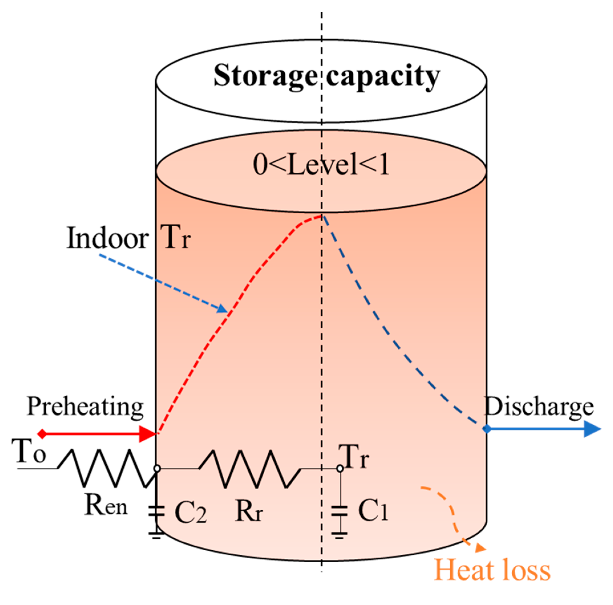
3.2.2. Virtual Thermal Energy Storage
4. Results and Discussions
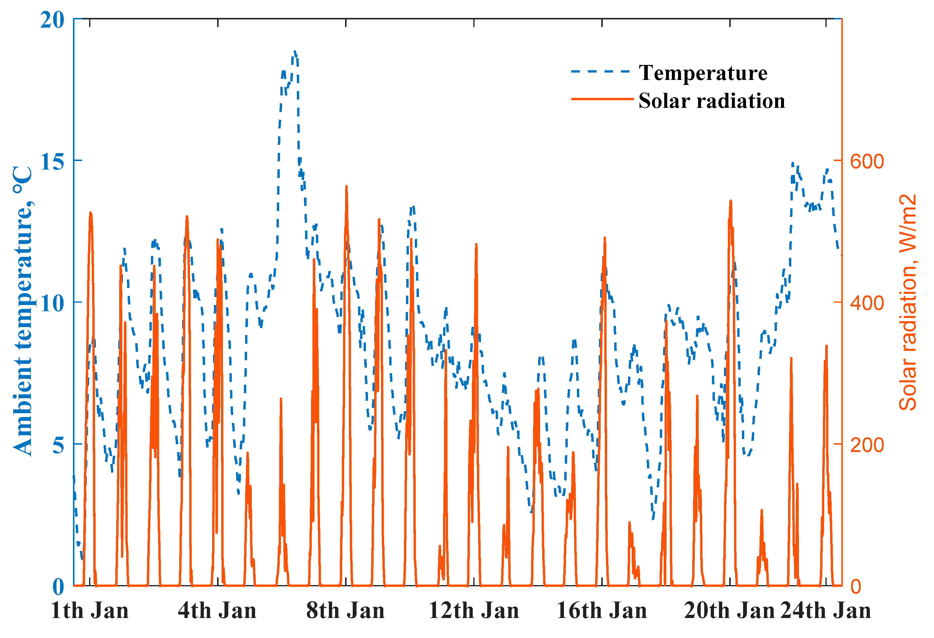
4.1. Measured Operational Performances
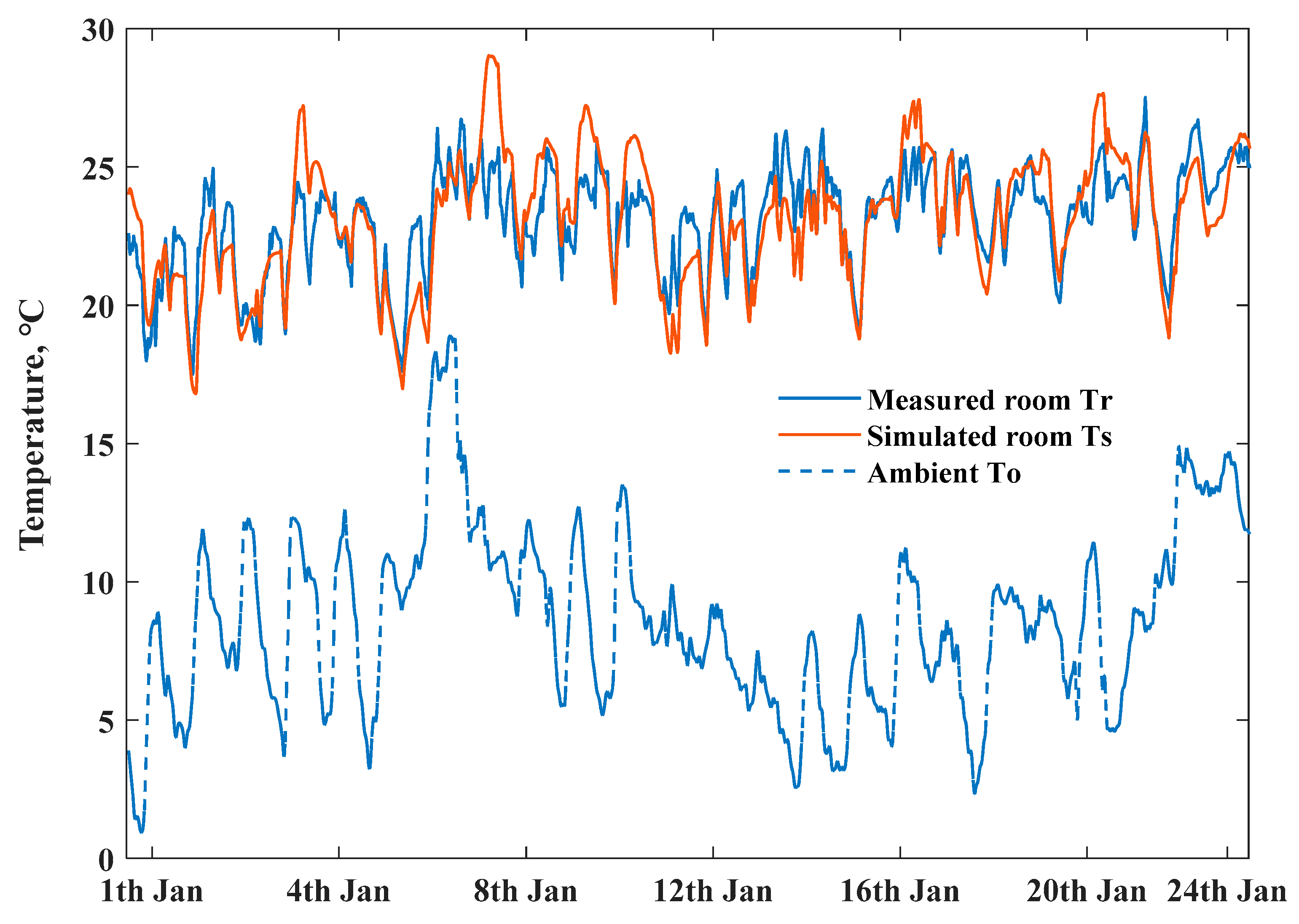
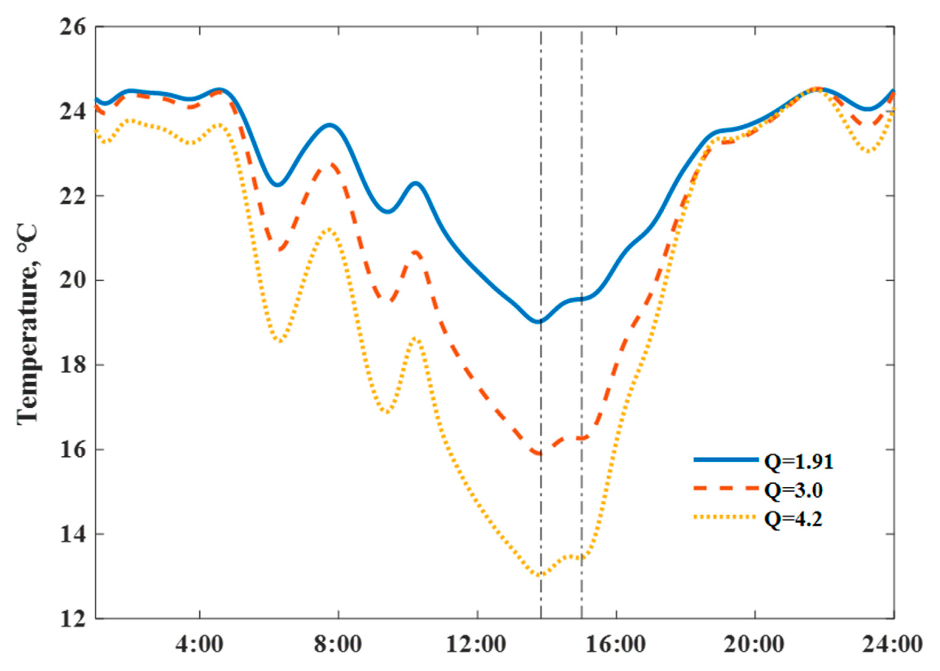
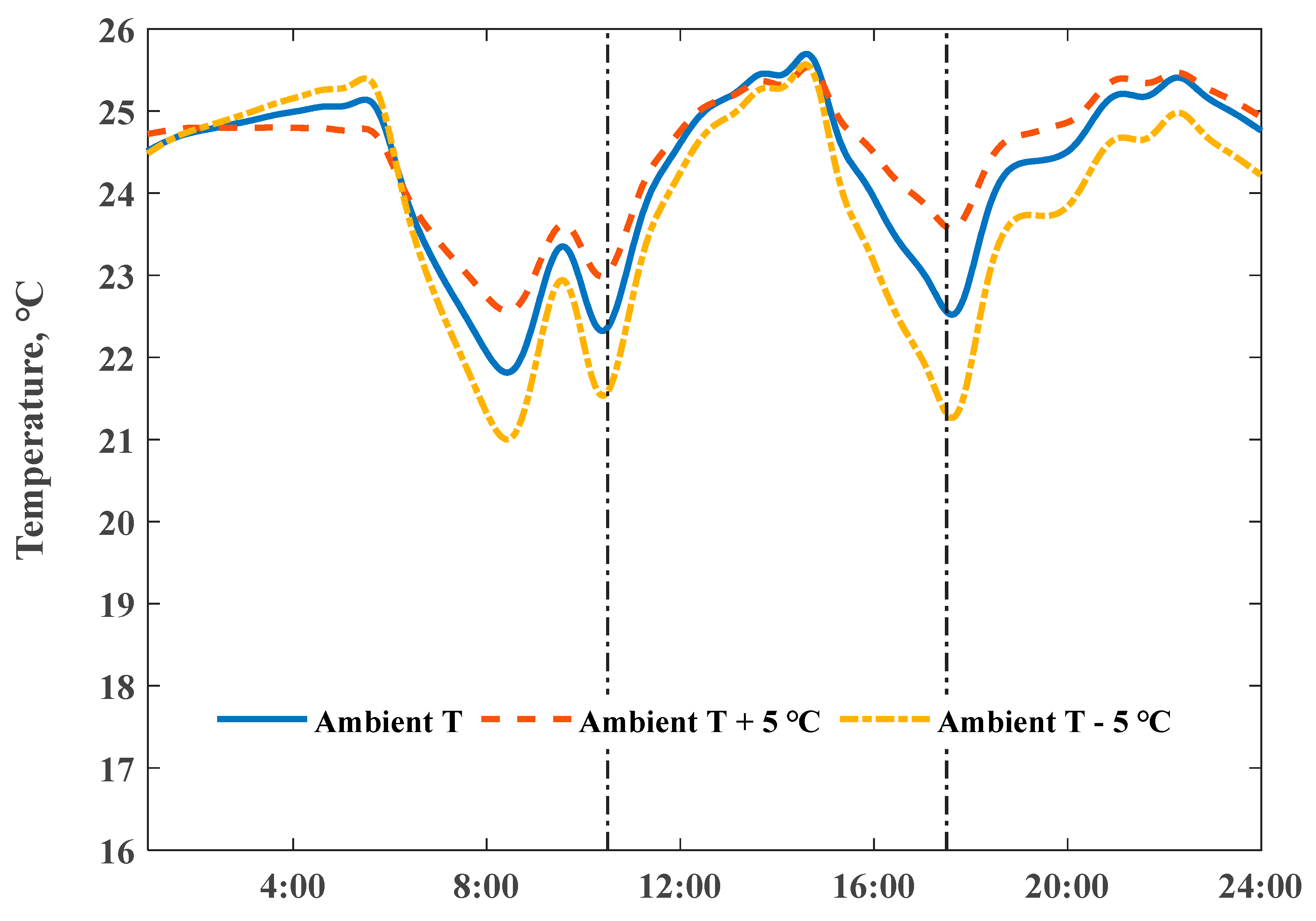
4.2. Simulation Results
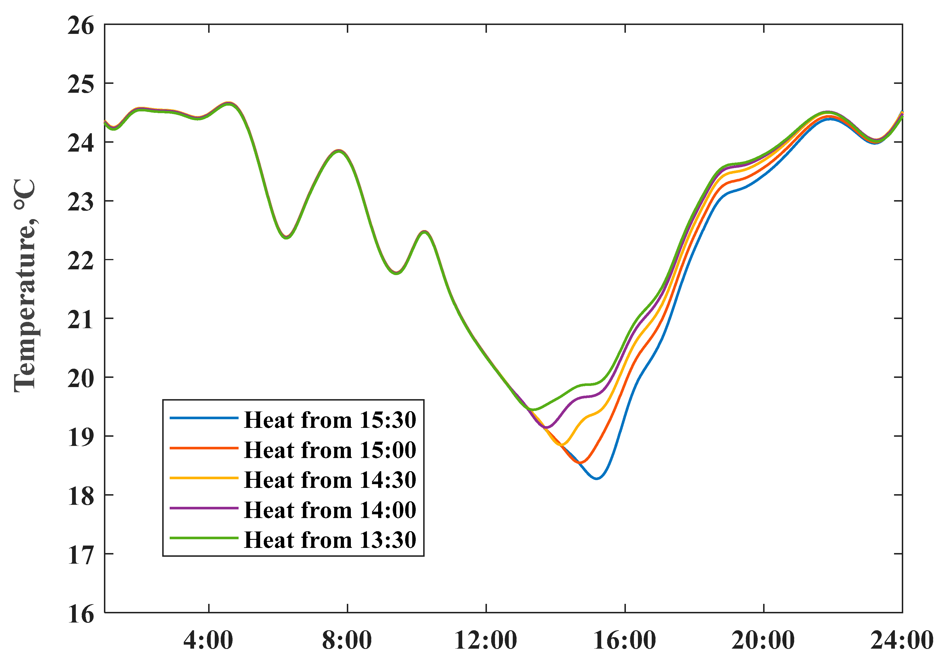
4.3. Operational Load Flexibility
4.4. Load Shift Potential
5. Conclusions
Author Contributions
Funding
Institutional Review Board Statement
Informed Consent Statement
Data Availability Statement
Acknowledgments
Conflicts of Interest
Nomenclature
| Aen | Total envelope area, m2 |
| Afloor | House floor area, m2 |
| C1 | Room air heat capacity, kJ/K |
| C2 | Envelope heat capacity, kJ/K |
| Ua | Thermal transmittance of the envelope, W/(m2*K) |
| Q | Building heat loss coefficient, W/(m2*K) |
| Qen | Overall envelope heat energy loss per degree, W/K |
| Qven | Ventilation heat energy loss per degree, W/K |
| Io | Solar radiation, W/m2 |
| qrw | Heat flow from the room to the envelope, W/m2 |
| qen | Heat flow from the envelope to the outside, W/m2 |
| q | Indoor heat energy gain, W/m2 |
| Rr | Thermal resistance between room air and exposed indoor thermal mass, (m2*K)/W |
| Ren | Overall thermal resistance between envelope and outdoor air and ventilation, (m2*K)/W |
| ho | Coefficient of heat transfer of out surface, W/(m2*K) |
| To | Ambient temperature, °C |
| Ten | Envelope temperature, °C |
| Tr | Room air temperature, °C |
| Tso | Solar air equivalent temperature, °C |
| Vair | Room air volume, m3 |
| Ven | Room envelope volume, m3 |
| cair | The specific air heat capacity, J(kg*K) |
| cen | The specific envelope heat capacity, J(kg*K) |
| mair | Indoor air mass, kg |
| men | Envelope mass, kg |
| Solar radiation absorptivity factor | |
| ρair | Air density, kg/m3 |
| ρen | Overall envelope density, kg/m3 |
| ZEH | Zero energy house |
| PV | Photovoltaic |
References
- Oki, R.; Tsuneoka, Y.; Yamaguchi, S.; Sugano, S.; Watanabe, N.; Akimoto, T.; Hayashi, Y.; Wakao, S.; Tanabe, S.-I. Renovating a house to aim for net-zero energy, thermal comfort, energy self-consumption and behavioural adaptation: A method proposed for enemane house 2017. Energy Build. 2019, 201, 183–193. [Google Scholar] [CrossRef]
- Li, Y.; Gao, W.; Zhang, X.; Ruan, Y.; Ushifusa, Y.; Hiroatsu, F. Techno-economic performance analysis of zero energy house applications with home energy management system in Japan. Energy Build. 2020, 214, 109862. [Google Scholar] [CrossRef]
- Stinner, S.; Huchtemann, K.; Müller, D. Quantifying the operational flexibility of building energy systems with thermal energy storages. Appl. Energy 2016, 181, 140–154. [Google Scholar] [CrossRef]
- Wang, H.; Wang, S.; Tang, R. Development of grid-responsive buildings: Opportunities, challenges, capabilities and applications of HVAC systems in non-residential buildings in providing ancillary services by fast demand responses to smart grids. Appl. Energy 2019, 250, 697–712. [Google Scholar] [CrossRef]
- Li, Y.; Gao, W.; Ruan, Y. Performance investigation of grid-connected residential PV-battery system focusing on enhancing self-consumption and peak shaving in Kyushu, Japan. Renew. Energy 2018, 127, 514–523. [Google Scholar] [CrossRef]
- Le Dréau, J.; Heiselberg, P. Energy flexibility of residential buildings using short term heat storage in the thermal mass. Energy 2016, 111, 991–1002. [Google Scholar] [CrossRef]
- Klein, K.; Herkel, S.; Henning, H.-M.; Felsmann, C. Load shifting using the heating and cooling system of an office building: Quantitative potential evaluation for different flexibility and storage options. Appl. Energy 2017, 203, 917–937. [Google Scholar] [CrossRef]
- Tulabing, R.; Yin, R.; DeForest, N.; Li, Y.; Wang, K.; Yong, T.; Stadler, M. Modeling study on flexible load’s demand response potentials for providing ancillary services at the substation level. Electr. Power Syst. Res. 2016, 140, 240–252. [Google Scholar] [CrossRef] [Green Version]
- Sweetnam, T.; Fell, M.; Oikonomou, E.; Oreszczyn, T. Domestic demand-side response with heat pumps: Controls and tariffs. Build. Res. Inf. 2018, 47, 344–361. [Google Scholar] [CrossRef] [Green Version]
- Taibi, E.; Nikolakakis, T.; Gutierrez, L.; Fernandez, C.; Kiviluoma, J.; Rissanen, S.; Lindroos, T.J. Power System Flexibility for the Energy Transition: Part 1, Overview for Policy Makers; International Renewable Energy Agency IRENA: Abu Dhabi, United Arab Emirates, 2018. [Google Scholar]
- Li, P.-H.; Pye, S. Assessing the benefits of demand-side flexibility in residential and transport sectors from an integrated energy systems perspective. Appl. Energy 2018, 228, 965–979. [Google Scholar] [CrossRef]
- Olivella-Rosell, P.; Lloret-Gallego, P.; Munné-Collado, Í.; Villafafila-Robles, R.; Sumper, A.; Ottessen, S.; Rajasekharan, J.; Bremdal, B. Local flexibility market design for aggregators providing multiple flexibility services at distribution network level. Energies 2018, 11, 822. [Google Scholar] [CrossRef] [Green Version]
- Ansarin, M.; Ghiassi-Farrokhfal, Y.; Ketter, W.; Collins, J. The economic consequences of electricity tariff design in a renewable energy era. Appl. Energy 2020, 275, 115317. [Google Scholar] [CrossRef]
- Lin, Y.; Zhong, S.; Yang, W.; Hao, X.; Li, C.-Q. Towards zero-energy buildings in China: A systematic literature review. J. Clean. Prod. 2020, 276, 123297. [Google Scholar] [CrossRef]
- Esbensen, T.V.; Korsgaard, V. Dimensioning of the solar heating system in the zero energy house in Denmark. Sol. Energy 1977, 19, 195–199. [Google Scholar] [CrossRef]
- Yu, Z.; Gou, Z.; Qian, F.; Fu, J.; Tao, Y. Towards an optimized zero energy solar house: A critical analysis of passive and active design strategies used in Solar Decathlon Europe in Madrid. J. Clean. Prod. 2019, 236, 117646. [Google Scholar] [CrossRef]
- Kosonen, A.; Keskisaari, A. Zero-energy log house—Future concept for an energy efficient building in the Nordic conditions. Energy Build. 2020, 228, 110449. [Google Scholar] [CrossRef]
- Vieira, F.M.; Moura, P.S.; de Almeida, A.T. Energy storage system for self-consumption of photovoltaic energy in residential zero energy buildings. Renew. Energy 2017, 103, 308–320. [Google Scholar] [CrossRef]
- Wang, R.; Feng, W.; Wang, L.; Lu, S. A comprehensive evaluation of zero energy buildings in cold regions: Actual performance and key technologies of cases from China, the US, and the European Union. Energy 2021, 215, 118992. [Google Scholar] [CrossRef]
- Schill, W.-P.; Zerrahn, A. Flexible electricity use for heating in markets with renewable energy. Appl. Energy 2020, 266, 114571. [Google Scholar] [CrossRef]
- Li, Y.; Zhang, X.; Gao, W.; Ruan, Y. Capacity credit and market value analysis of photovoltaic integration considering grid flexibility requirements. Renew. Energy 2020, 159, 908–919. [Google Scholar] [CrossRef]
- Vigna, I.; Pernetti, R.; Pasut, W.; Lollini, R. New domain for promoting energy efficiency: Energy flexible building cluster. Sustain. Cities Soc. 2018, 38, 526–533. [Google Scholar] [CrossRef]
- Jensen, S.Ø.; Marszal-Pomianowska, A.; Lollini, R.; Pasut, W.; Knotzer, A.; Engelmann, P.; Stafford, A.; Reynders, G. IEA EBC annex 67 energy flexible buildings. Energy Build. 2017, 155, 25–34. [Google Scholar] [CrossRef] [Green Version]
- Bechtel, S.; Rafii-Tabrizi, S.; Scholzen, F.; Hadji-Minaglou, J.-R.; Maas, S. Influence of thermal energy storage and heat pump parametrization for demand-side-management in a nearly-zero-energy-building using model predictive control. Energy Build. 2020, 226, 110364. [Google Scholar] [CrossRef]
- Fitzpatrick, P.; D’Ettorre, F.; De Rosa, M.; Yadack, M.; Eicker, U.; Finn, D.P. Influence of electricity prices on energy flexibility of integrated hybrid heat pump and thermal storage systems in a residential building. Energy Build. 2020, 223, 110142. [Google Scholar] [CrossRef]
- Li, Y.; Gao, W.; Ruan, Y.; Ushifusa, Y. Demand response of customers in Kitakyushu smart community project to critical peak pricing of electricity. Energy Build. 2018, 168, 251–260. [Google Scholar] [CrossRef]
- Shen, L.; Li, Z.; Sun, Y. Performance evaluation of conventional demand response at building-group-level under different electricity pricings. Energy Build. 2016, 128, 143–154. [Google Scholar] [CrossRef]
- Yu, Z.; Lu, F.; Zou, Y.; Yang, X. Quantifying the flexibility of lighting systems by optimal control in commercial buildings: Insight from a case study. Energy Build. 2020, 225, 110310. [Google Scholar] [CrossRef]
- Barone, G.; Buonomano, A.; Forzano, C.; Giuzio, G.F.; Palombo, A. Increasing self-consumption of renewable energy through the building to vehicle to building approach applied to multiple users connected in a virtual micro-grid. Renew. Energy 2020, 159, 1165–1176. [Google Scholar] [CrossRef]
- Georges, E.; Cornélusse, B.; Ernst, D.; Lemort, V.; Mathieu, S. Residential heat pump as flexible load for direct control service with parametrized duration and rebound effect. Appl. Energy 2017, 187, 140–153. [Google Scholar] [CrossRef] [Green Version]
- Williams, S.; Short, M.; Crosbie, T. On the use of thermal inertia in building stock to leverage decentralised demand side frequency regulation services. Appl. Therm. Eng. 2018, 133, 97–106. [Google Scholar] [CrossRef] [Green Version]
- Asadinejad, A.; Rahimpour, A.; Tomsovic, K.; Qi, H.; Chen, C.-F. Evaluation of residential customer elasticity for incentive based demand response programs. Electr. Power Syst. Res. 2018, 158, 26–36. [Google Scholar] [CrossRef]
- Violante, W.; Canizares, C.A.; Trovato, M.A.; Forte, G. An energy management system for isolated microgrids with thermal energy resources. IEEE Trans. Smart Grid 2020, 11, 2880–2891. [Google Scholar]
- Chassin, D.P.; Stoustrup, J.; Agathoklis, P.; Djilali, N. A new thermostat for real-time price demand response: Cost, comfort and energy impacts of discrete-time control without deadband. Appl. Energy 2015, 155, 816–825. [Google Scholar] [CrossRef] [Green Version]
- Short, M.; Rodriguez, S.; Charlesworth, R.; Crosbie, T.; Dawood, N. Optimal dispatch of aggregated HVAC units for demand response: An industry 4.0 approach. Energies 2019, 12, 4320. [Google Scholar] [CrossRef] [Green Version]
- Danza, L.; Belussi, L.; Meroni, I.; Salamone, F.; Floreani, F.; Piccinini, A.; Dabusti, A. A simplified thermal model to control the energy fluxes and to improve the performance of buildings. Energy Procedia 2016, 101, 97–104. [Google Scholar] [CrossRef]
- Ghiaus, C.; Ahmad, N. Thermal circuits assembling and state-space extraction for modelling heat transfer in buildings. Energy 2020, 195, 117019. [Google Scholar]
- Hurwitz, Z.L.; Dubief, Y.; Almassalkhi, M. Economic efficiency and carbon emissions in multi-energy systems with flexible buildings. Int. J. Electr. Power Energy Syst. 2020, 123, 106114. [Google Scholar]
- Weiß, T.; Fulterer, A.M.; Knotzer, A. Energy flexibility of domestic thermal loads—A building typology approach of the residential building stock in Austria. Adv. Build. Energy Res. 2018, 13, 122–137. [Google Scholar]
- Jin, X.; Mu, Y.; Jia, H.; Wu, J.; Jiang, T.; Yu, X. Dynamic economic dispatch of a hybrid energy microgrid considering building based virtual energy storage system. Appl. Energy 2017, 194, 386–398. [Google Scholar]
- Masy, G.; Georges, E.; Verhelst, C.; Lemort, V.; André, P. Smart grid energy flexible buildings through the use of heat pumps and building thermal mass as energy storage in the Belgian context. Sci. Technol. Built Environ. 2015, 21, 800–811. [Google Scholar]
- Oliveira Panão, M.J.N.; Mateus, N.M.; Carrilho da Graça, G. Measured and modeled performance of internal mass as a thermal energy battery for energy flexible residential buildings. Appl. Energy 2019, 239, 252–267. [Google Scholar] [CrossRef]
- Reynders, G.; Amaral Lopes, R.; Marszal-Pomianowska, A.; Aelenei, D.; Martins, J.; Saelens, D. Energy flexible buildings: An evaluation of definitions and quantification methodologies applied to thermal storage. Energy Build. 2018, 166, 372–390. [Google Scholar] [CrossRef]
- Kamel, E.; Iuldasheva, A. The Effectiveness of HVAC Demand Response Control on Buildings with Low and High Thermal Insulation. In Proceedings of the 2019 Buildings XIV International Conference, Clearwater Beach, FL, USA, 9–12 December 2019. [Google Scholar]
- Balint, A.; Kazmi, H. Determinants of energy flexibility in residential hot water systems. Energy Build. 2019, 188–189, 286–296. [Google Scholar] [CrossRef]
- Ulbig, A.; Andersson, G. Analyzing operational flexibility of electric power systems. Int. J. Electr. Power Energy Syst. 2015, 72, 155–164. [Google Scholar] [CrossRef]
- Kathirgamanathan, A.; Péan, T.; Zhang, K.; De Rosa, M.; Salom, J.; Kummert, M.; Finn, D.P. Towards standardising market-independent indicators for quantifying energy flexibility in buildings. Energy Build. 2020, 220, 110027. [Google Scholar] [CrossRef]
- Harder, N.; Qussous, R.; Weidlich, A. The cost of providing operational flexibility from distributed energy resources. Appl. Energy 2020, 279, 115784. [Google Scholar] [CrossRef]
- De Coninck, R.; Helsen, L. Quantification of flexibility in buildings by cost curves—Methodology and application. Appl. Energy 2016, 162, 653–665. [Google Scholar] [CrossRef]
- Junker, R.G.; Azar, A.G.; Lopes, R.A.; Lindberg, K.B.; Reynders, G.; Relan, R.; Madsen, H. Characterizing the energy flexibility of buildings and districts. Appl. Energy 2018, 225, 175–182. [Google Scholar] [CrossRef]
- Institute, H.P.D. Investigation of the Relationship between House Q and UA Value; House Performance Diagnosis Institute: Atlanta, GA, USA, 2018. [Google Scholar]
- Al-Saud, K.A. Measured versus calculated roof peak sol-air temperature in hot-arid regions. Red 2009, 29, 95. [Google Scholar]
- Tuck, N.W.; Zaki, S.A.; Hagishima, A.; Rijal, H.B.; Yakub, F. Affordable retrofitting methods to achieve thermal comfort for a terrace house in Malaysia with a hot–humid climate. Energy Build. 2020, 223, 110072. [Google Scholar] [CrossRef]
- Ministry of Economy, Trade and Industry. Feed in Tariff for Renewable Energy in Japan. Available online: https://www.meti.go.jp/shingikai/santeii/pdf/063_01_00.pdf (accessed on 1 November 2020).


| Established Year | 2017 |
|---|---|
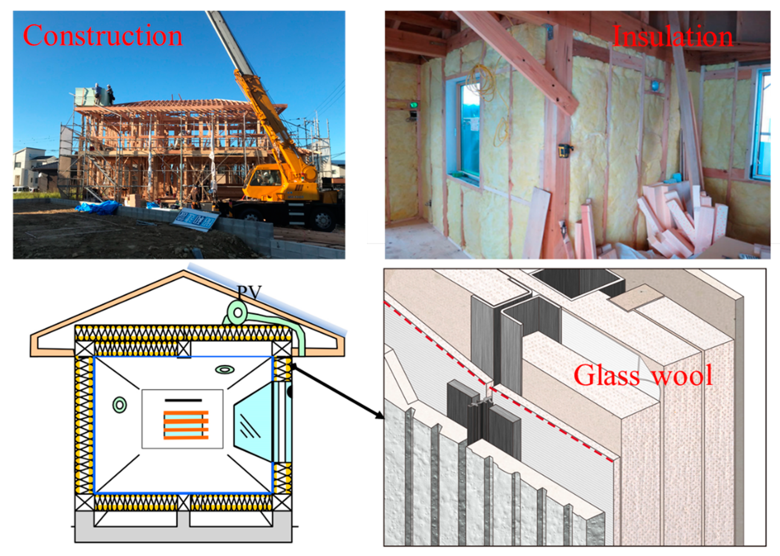
| Structural material | Lightweight steel and wooden skeleton, infill structure, 2 stories |
| Envelope heat loss coefficient | : 1.91 W/(m2 K), : 0.58 W/(m2 K) |
| Thermal insulation material and characteristic | Wall: glass wool 120 mm and glass board 12 mm; roof: glass wall 100 mm; floor: glass wall 67 mm; thermal conductivity 0.04 W/(m K) |
| Ventilation rate | Mechanical ventilation, 0.5 ac/h |
| Window | Low-E pair glass with plastic combined aluminum sash |
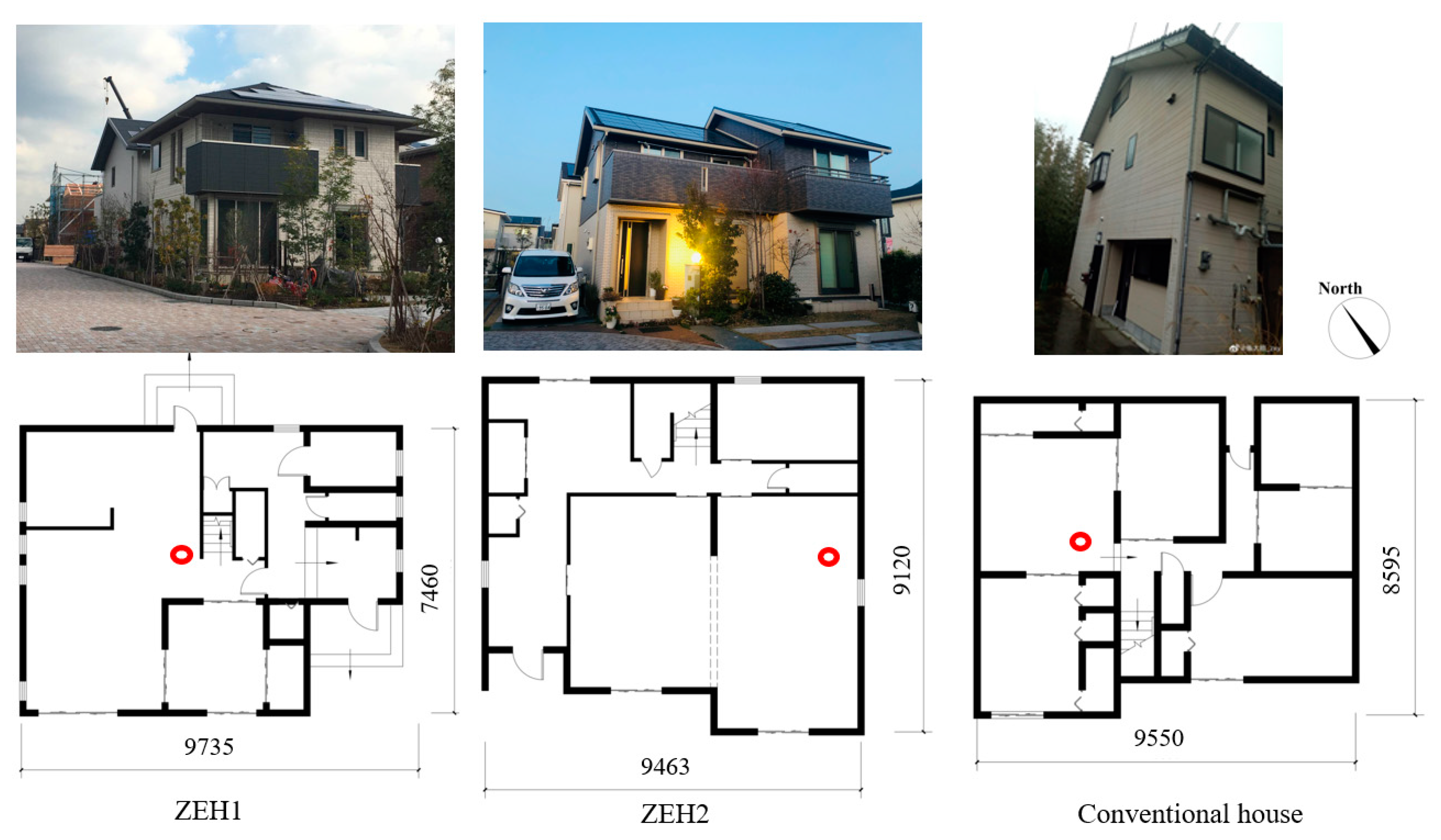
| Window-to-wall ratio | ZEH 1: 0.16, ZEH 2: 0.18 |
| Variables | Room Air Volume, m3 | Structure Volume, m3 | C1, kJ/K | C2, kJ/K |
|---|---|---|---|---|
| Value | 210 | 8 | 2540 | 5000 |
| Variables | From 15:00 | From 14:30 | From 14:00 | From 13:30 |
|---|---|---|---|---|
| Preheat power input (PV generation), Wh | 498 | 897 | 1230 | 1463 |
| Amount of replaced heating power, Wh | 201 | 433 | 665 | 839 |
Publisher’s Note: MDPI stays neutral with regard to jurisdictional claims in published maps and institutional affiliations. |
© 2021 by the authors. Licensee MDPI, Basel, Switzerland. This article is an open access article distributed under the terms and conditions of the Creative Commons Attribution (CC BY) license (https://creativecommons.org/licenses/by/4.0/).
Share and Cite
Zhang, X.; Gao, W.; Li, Y.; Wang, Z.; Ushifusa, Y.; Ruan, Y. Operational Performance and Load Flexibility Analysis of Japanese Zero Energy House. Int. J. Environ. Res. Public Health 2021, 18, 6782. https://0-doi-org.brum.beds.ac.uk/10.3390/ijerph18136782
Zhang X, Gao W, Li Y, Wang Z, Ushifusa Y, Ruan Y. Operational Performance and Load Flexibility Analysis of Japanese Zero Energy House. International Journal of Environmental Research and Public Health. 2021; 18(13):6782. https://0-doi-org.brum.beds.ac.uk/10.3390/ijerph18136782
Chicago/Turabian StyleZhang, Xiaoyi, Weijun Gao, Yanxue Li, Zixuan Wang, Yoshiaki Ushifusa, and Yingjun Ruan. 2021. "Operational Performance and Load Flexibility Analysis of Japanese Zero Energy House" International Journal of Environmental Research and Public Health 18, no. 13: 6782. https://0-doi-org.brum.beds.ac.uk/10.3390/ijerph18136782