
Non-Linear Effects of the Built Environment and Social Environment on Bus Use among Older Adults in China: An Application of the XGBoost Model

 ,
,
Abstract
:1. Introduction
2. Literature Review

| Study | Sample (Area) | Dependent Variables | Built Environment | Method |
|---|---|---|---|---|
| Vergel-Tovar and Rodriguez [49] | 120 BRT stations in seven cities (Colombia, Brazil, Guatemala, and Ecuador in Latin American) | BRT ridership | Density, Diversity, Design, Destination accessibility | Factor analysis, Cluster analysis, Log-linear regression |
| Li et al. [58] | 124 subway stations (Guangzhou, China) | Rail transit ridership | Density, Diversity, Station characteristics | Geographically weighted regression (GWR), K-means clustering |
| Lin, Weng, Brands, Qian, and Yin [51] | 1151 TAZs in the Sixth Ring Road of Beijing (Beijing, China) | Public transport ridership | Density, Design, Diversity, Distance | Light Gradient Boosted Machine (LightGBM) |
| Chakour and Eluru [59] | 8000 stops in Montreal the ridership (Montreal, Canada) | Boardings/ Alightings per hour | Design, Distance to transit, Diversity, Destination accessibility | Composite Marginal Likelihood (CML)-based ordered response probit (ORP) model |
| Chen et al. [60] | Four weeks of smart card data (Nanjing, China) | Intermodal transit trips (bus and metro) | Density, Diversity, Design, Distance to transit, Destination accessibility | Traditional random forest incorporates the GWR model |
| De Gruyter et al. [61] | 10,289 SA1s in Metropolitan Melbourne (Melbourne, Australia) | Commuting trips by transit/ train/ tram/bus (all modes) | Density, Diversity, Design, Destination accessibility, Distance to transit, Demand management | Ordinary least squares (OLS), Beta regression |
| Yang, Xu, Rodriguez, Michael, and Zhang [46] | 75,862 older adults; 104,613 adults aged between 45 and 64 (U.S.) | Public transport trips | Design, Destination accessibility | Linear regression, Logistic regression |
| Zhao et al. [62] | Approximately 3,000,000 daily card-swiping records of transit users in March 2015 (Wuhan, China) | Transit trip rates | Density, Diversity, Distance to the bus stop, Distance to the destination | Bilevel hierarchical linear model (HLM) |
| Liu et al. [63] | Go card data containing trip transactions of all commuters using bus, train, and ferry services for two one-week periods (21–27 March 2016 under the old fare policy, and 20–26 March 2017 under the new fare policy) (South East Queensland, Australia) | The change in public transport ridership | Diversity, Density, Destination accessibility, Distance, | Spatial lag regression (SLR) |
| Ding, Cao, Yu, and Ju [52] | 3758 commuters (Nanjing, China) | Transit commuting mode choice | Density, Diversity, Design, Destination accessibility, Distance to CBD | Semi-parametric multilevel mixed logit model |
| Yu, Xie, and Chan [50] | 565 respondents from urban villages; 985 respondents from formal residences (Shenzhen, China) | Public transit choice | Density, Diversity, Distance to transit | Multinomial logistic regression (MNL) |
| Pongprasert and Kubota [64] | 477 respondents (online questionnaire: 160; on-the-road survey: 317) (Bangkok, Thailand) | The probability with which car users’ switch to transit | Destination, Distance, Diversity, Density, Design, Demand management | Binary logistic regression model |
3. Data
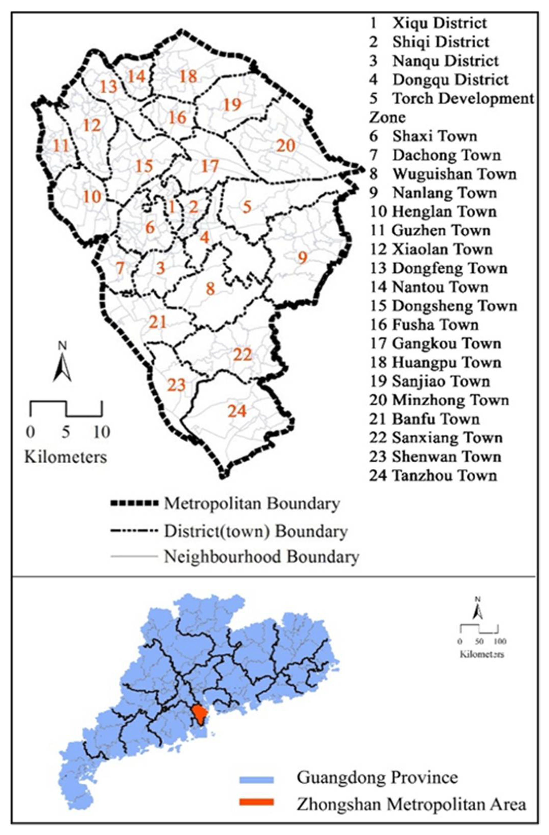
3.1. Study Area
3.2. Data Collection
3.3. Variables
3.3.1. Characterization of Personal, Attitudinal, and Household Variables
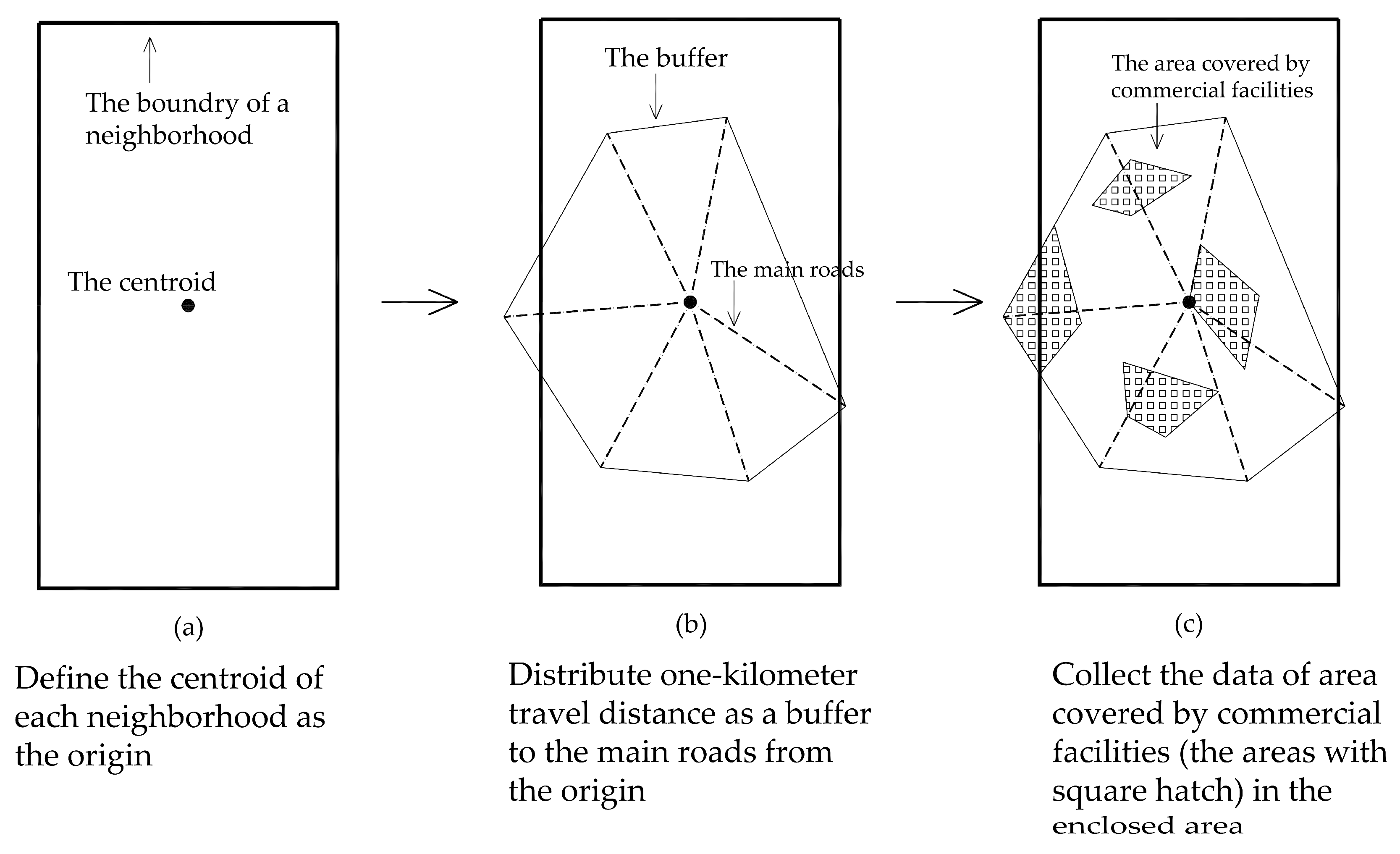
3.3.2. Characterization of Social Environment and Built Environment Variables
- Define the centroid of each neighborhood as the origin,
- Distribute a one kilometer travel distance as a buffer to the main roads from the origin,
- Form an enclosed area with the endpoints of the acceptable travel distances in ArcGIS,
- Collect the data of the area covered by commercial facilities in the enclosed area in ArcGIS,
- Divide the data by the population of the neighborhood to obtain the commercial accessibility.
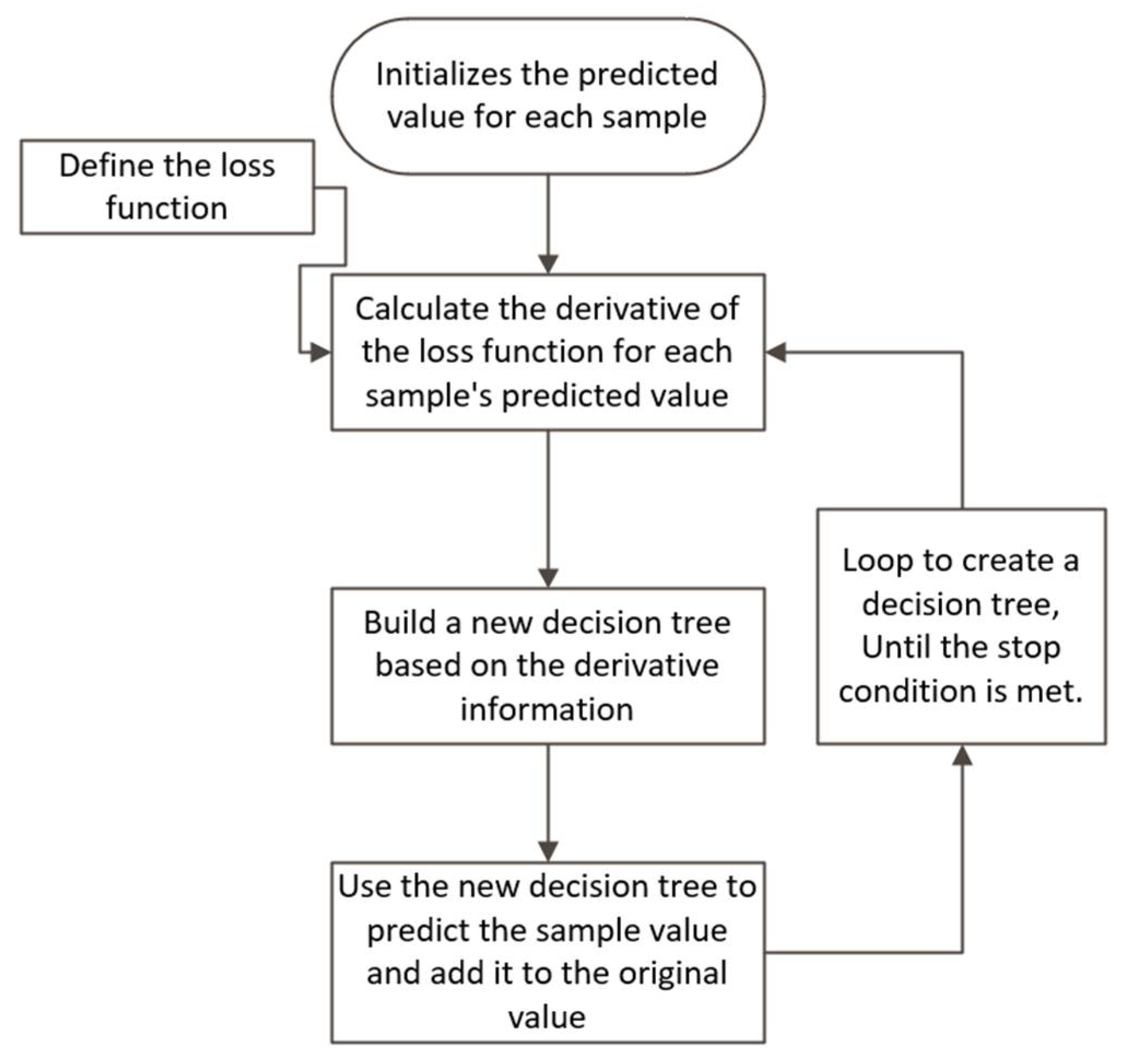
4. Method
- Regularization term: XGBoost adds the regularization term to control the complexity of the model. It helps to prevent overfitting and improve the generalization ability of the model.
- Second-order derivative: GBDT only uses the first-order derivative information of the cost function in the model training. XGBoost performs a second-order Taylor expansion on the cost function, and both the first and second derivatives can be used.
- Column sampling: The traditional GBDT uses all the data in each iteration. XGBoost uses a strategy similar to the random forest. It supports data sampling and column sampling, which not only reduces overfitting, but also reduces calculations.
- Missing value processing: The traditional GBDT is not designed to deal with missing values. XGBoost can automatically learn its splitting direction.
5. Results and Discussion
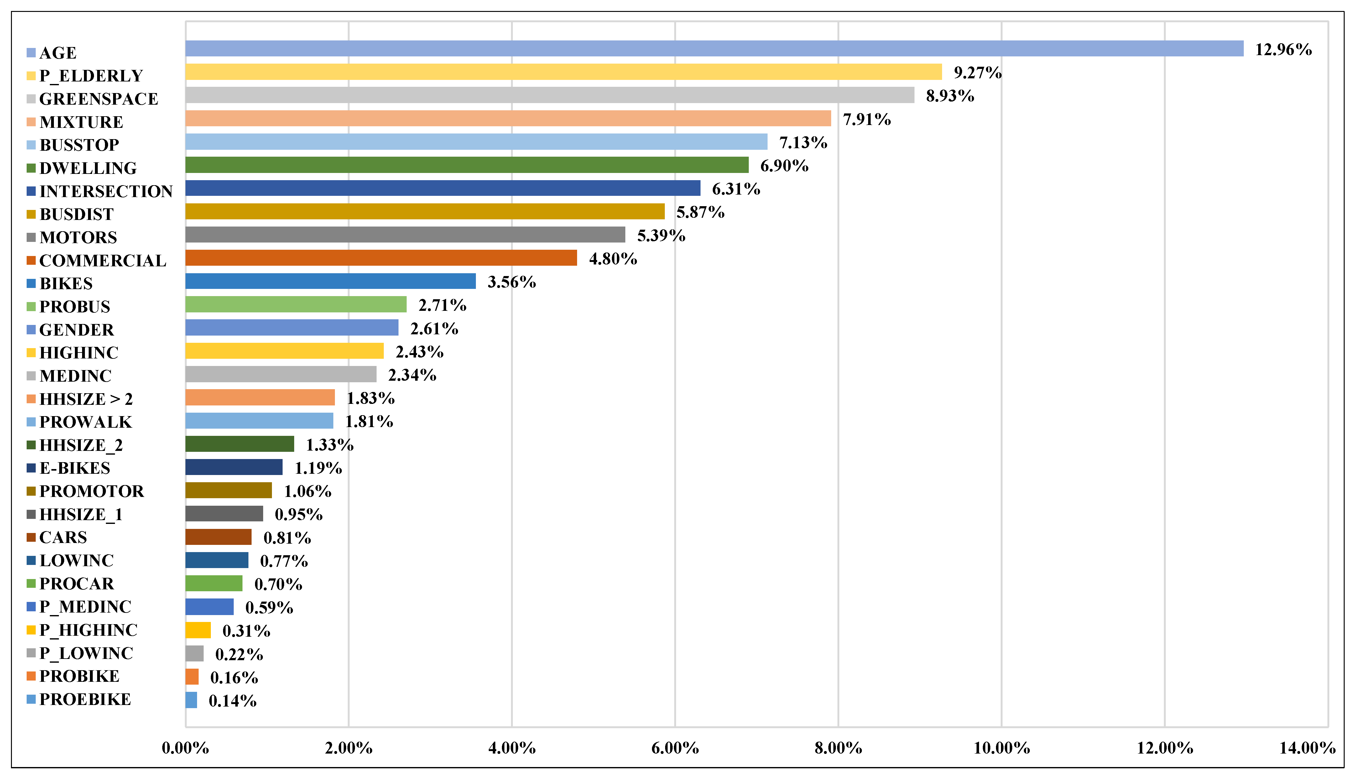
5.1. Relative Importance of Independent Variables
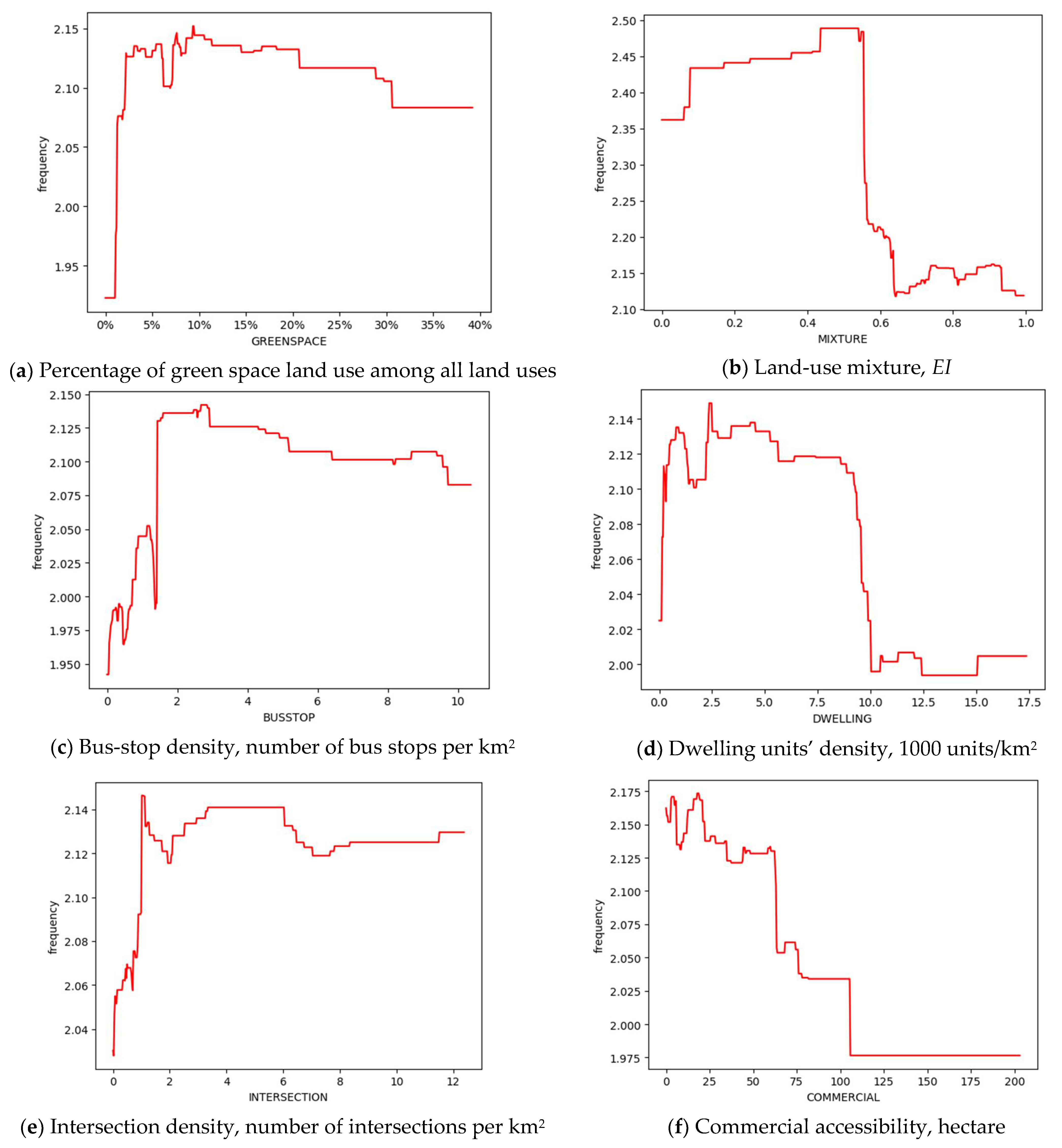
5.2. Non-Linear Relationships with Built Environment Variables
5.2.1. Non-Linear Relationship with the Percentage of Green Space Land Use
5.2.2. Non-Linear Relationship with the Land Use Mixture
5.2.3. Non-Linear Relationship with the Percentage of Bus-Stop Density
5.2.4. Non-Linear Relationship with the Dwelling Unit Density
5.3. Non-Linear Relationships with Key Social Environment Variable
5.4. Non-Linear Relationships with Key Personal and Household Variables
5.4.1. Non-Linear Relationships with Key Personal Variables
5.4.2. Non-Linear Relationships with Key Household Variables
5.5. Model Comparison
5.5.1. The Improvement of the XGBoost Model
5.5.2. The Performance of the XGBoost Model
6. Conclusions
Author Contributions
Funding
Institutional Review Board Statement
Informed Consent Statement
Data Availability Statement
Conflicts of Interest
References
- Population Ageing 2020 Highlights: Living Arrangements of Older Persons; ST/ESA/SER.A/451; United Nations Department of Economic and Social Affairs, Population Division. Available online: https://www.un.org/development/desa/pd/sites/www.un.org.development.desa.pd/files/undesa_pd-2020_world_population_ageing_highlights.pdf (accessed on 10 September 2021).
- United Nations Department of Economic and Social Affairs, Population Division. 2020. Ten Key Messages. Available online: https://www.un.org/development/desa/pd/sites/www.un.org.development.desa.pd/files/international_migration_2020_highlights_ten_key_messages.pdf (accessed on 10 September 2021).
- SDG 3 U.N. 17 Goals to Transform Our World, Goal 3: Ensure Healthy Lives and Promote Well-Being for all at all Ages. Available online: https://www.un.org/sustainabledevelopment/sustainable-development-goals/ (accessed on 20 March 2021).
- Szeto, W.; Yang, L.; Wong, R.; Li, Y.; Wong, S.C. Spatio-temporal travel characteristics of the elderly in an ageing society. Travel Behav. Soc. 2017, 9, 10–20. [Google Scholar] [CrossRef] [Green Version]
- Aceves-González, C.; Cook, S.; May, A. Bus use in a developing world city: Implications for the health and well-being of older passengers. J. Transp. Heal. 2015, 2, 308–316. [Google Scholar] [CrossRef] [Green Version]
- Webber, M.S.C.; Porter, M.M.; Menec, V.H. Mobility in Older Adults: A Comprehensive Framework. Gerontologist 2010, 50, 443–450. [Google Scholar] [CrossRef] [Green Version]
- Yeom, H.A.; Fleury, J.; Keller, C. Risk Factors for Mobility Limitation in Community-Dwelling Older Adults: A Social Ecological Perspective. Geriatr. Nurs. 2008, 29, 133–140. [Google Scholar] [CrossRef] [PubMed]
- Giuliano, G. Low income, public transit, and mobility. Transit: Planning, Management and Maintenance, Technology, Marketing and Fare Policy, and Capacity and Qualtiy of Sevice. Transp. Res. Rec. Ser. 2005, 1927, 63–70. [Google Scholar] [CrossRef]
- Duvarci, Y.; Yigitcanlar, T. Integrated Modeling Approach for the Transportation Disadvantaged. J. Urban Plan. Dev. 2007, 133, 188–200. [Google Scholar] [CrossRef] [Green Version]
- Cheng, L.; Chen, X.; Yang, S.; Cao, Z.; De Vos, J.; Witlox, F. Active travel for active ageing in China: The role of built environment. J. Transp. Geogr. 2019, 76, 142–152. [Google Scholar] [CrossRef]
- Musselwhite, C.; Holland, C.; Walker, I. The role of transport and mobility in the health of older people. J. Transp. Health 2015, 2, 1–4. [Google Scholar] [CrossRef] [Green Version]
- Voss, C.; Gould, J.S.; Ashe, M.C.; McKay, H.A.; Pugh, C.; Winters, M. Public transit use and physical activity in community-dwelling older adults: Combining GPS and accelerometry to assess transportation-related physical activity. J. Transp. Health 2016, 3, 191–199. [Google Scholar] [CrossRef]
- Day, K.; Loh, L.; Ruff, R.R.; Rosenblum, R.; Fischer, S.; Lee, K.K. Does Bus Rapid Transit Promote Walking? An Examination of New York City’s Select Bus Service. J. Phys. Act. Health 2014, 11, 1512–1516. [Google Scholar] [CrossRef] [PubMed]
- Haselwandter, E.M.; Corcoran, M.P.; Folta, S.C.; Hyatt, R.; Nelson, M.E. The Built Environment, Physical Activity, and Aging in the United States: A State of the Science Review. J. Aging Phys. Act. 2015, 23, 323–329. [Google Scholar] [CrossRef]
- De Vos, J.; Schwanen, T.; Van Acker, V.; Witlox, F.; De Vos, J.; Schwanen, T.; Van Acker, V.; Witlox, F. Travel and Subjective Well-Being: A Focus on Findings, Methods and Future Research Needs. Transp. Rev. 2013, 33, 421–442. [Google Scholar] [CrossRef] [Green Version]
- Hayes, S.M.; Alosco, M.L.; Hayes, J.P.; Cadden, M.; Peterson, K.M.; Allsup, K.; Forman, D.E.; Sperling, R.A.; Verfaellie, M. Physical Activity Is Positively Associated with Episodic Memory in Aging. J. Int. Neuropsychol. Soc. 2015, 21, 780–790. [Google Scholar] [CrossRef] [PubMed] [Green Version]
- Sofi, F.; Valecchi, D.; Bacci, D.; Abbate, R.; Gensini, G.F.; Casini, A.; Macchi, C. Physical activity and risk of cognitive decline: A meta-analysis of prospective studies. J. Intern. Med. 2010, 269, 107–117. [Google Scholar] [CrossRef]
- Song, S.; Yap, W.; Hou, Y.; Yuen, B. Neighbourhood built Environment, physical activity, and physical health among older adults in Singapore: A simultaneous equations approach. J. Transp. Health 2020, 18, 100881. [Google Scholar] [CrossRef]
- Zhang, Y.; Li, Y.; Liu, Q.; Li, C. The Built Environment and Walking Activity of the Elderly: An Empirical Analysis in the Zhongshan Metropolitan Area, China. Sustainability 2014, 6, 1076–1092. [Google Scholar] [CrossRef] [Green Version]
- Lee, A. Gender, Everyday Mobility, and Mass Transit in Urban Asia. Mobil. Hist. 2017, 8, 85–93. [Google Scholar] [CrossRef]
- Yang, M.; Li, D.; Wang, W.; Zhao, J.; Chen, X. Modeling Gender-Based Differences in Mode Choice considering Time-Use Pattern: Analysis of Bicycle, Public Transit, and Car Use in Suzhou, China. Adv. Mech. Eng. 2013, 5, 706918. [Google Scholar] [CrossRef]
- Zhang, Y.; Wu, W.; He, Q.; Li, C. Public transport use among the urban and rural elderly in China: Effects of personal, attitudinal, household, social-environment and built-environment factors. J. Transp. Land Use 2018, 11, 701–719. [Google Scholar] [CrossRef]
- Chatman, D.G. Deconstructing development density: Quality, quantity and price effects on household non-work travel. Transp. Res. Part A Policy Pr. 2008, 42, 1008–1030. [Google Scholar] [CrossRef]
- Boarnet, M.G.; Greenwald, M.; Mcmillan, T.E. Walking, Urban Design, and Health: Toward a Cost-Benefit Analysis Framework. J. Plan. Educ. Res. 2008, 27, 341–358. [Google Scholar] [CrossRef]
- Boer, R.; Zheng, Y.; Overton, A.; Ridgeway, G.; Cohen, D.A. Neighborhood Design and Walking Trips in Ten U.S. Metropolitan Areas. Am. J. Prev. Med. 2007, 32, 298–304. [Google Scholar] [CrossRef] [PubMed] [Green Version]
- Ding, C.; Cao, X.; Næss, P. Applying gradient boosting decision trees to examine non-linear effects of the built environment on driving distance in Oslo. Transp. Res. Part A Policy Pr. 2018, 110, 107–117. [Google Scholar] [CrossRef]
- Ding, C.; Cao, X.; Liu, C. How does the station-area built environment influence Metrorail ridership? Using gradient boosting decision trees to identify non-linear thresholds. J. Transp. Geogr. 2019, 77, 70–78. [Google Scholar] [CrossRef]
- Yang, J.; Cao, J.; Zhou, Y. Elaborating non-linear associations and synergies of subway access and land uses with urban vitality in Shenzhen. Transp. Res. Part A: Policy Pr. 2020, 144, 74–88. [Google Scholar] [CrossRef]
- Tao, T.; Wang, J.; Cao, X. Exploring the non-linear associations between spatial attributes and walking distance to transit. J. Transp. Geogr. 2019, 82, 102560. [Google Scholar] [CrossRef]
- Cheng, L.; De Vos, J.; Zhao, P.; Yang, M.; Witlox, F. Examining non-linear built environment effects on elderly’s walking: A random forest approach. Transp. Res. Part D: Transp. Environ. 2020, 88, 102552. [Google Scholar] [CrossRef]
- Wu, J.; Zhao, C.; Li, C.; Wang, T.; Wang, L.; Zhang, Y. Non-linear Relationships Between the Built Environment and Walking Frequency Among Older Adults in Zhongshan, China. Front. Public Health 2021, 9, 1090. [Google Scholar] [CrossRef]
- Barnett, D.W.; Barnett, A.; Nathan, A.; Van Cauwenberg, J.; Cerin, E. Built environmental correlates of older adults’ total physical activity and walking: A systematic review and meta-analysis. Int. J. Behav. Nutr. Phys. Act. 2017, 14, 1–24. [Google Scholar] [CrossRef] [Green Version]
- Siu, V.W.; Lambert, W.E.; Fu, R.; Hillier, T.A.; Bosworth, M.; Michael, Y.L. Built Environment and Its Influences on Walking among Older Women: Use of Standardized Geographic Units to Define Urban Forms. J. Environ. Public Heal. 2012, 2012, 1–9. [Google Scholar] [CrossRef] [Green Version]
- Rodríguez, D.A.; Evenson, K.R.; Roux, A.V.D.; Brines, S.J. Land Use, Residential Density, and Walking: The Multi-Ethnic Study of Atherosclerosis. Am. J. Prev. Med. 2009, 37, 397–404. [Google Scholar] [CrossRef] [PubMed] [Green Version]
- Grimes, A.; Chrisman, M.; Lightner, J. Barriers and Motivators of Bicycling by Gender Among Older Adult Bicyclists in the Midwest. Heal. Educ. Behav. 2019, 47, 67–77. [Google Scholar] [CrossRef] [PubMed]
- Van Cauwenberg, J.; Clarys, P.; De Bourdeaudhuij, I.; Ghekiere, A.; de Geus, B.; Owen, N.; Deforche, B. Environmental influences on older adults’ transportation cycling experiences: A study using bike-along interviews. Landsc. Urban Plan. 2018, 169, 37–46. [Google Scholar] [CrossRef]
- Kemperman, A.; Timmermans, H. Influences of Built Environment on Walking and Cycling by Latent Segments of Aging Population. Transp. Res. Rec. J. Transp. Res. Board 2009, 2134, 1–9. [Google Scholar] [CrossRef]
- Prins, R.; Pierik, F.; Etman, A.; Sterkenburg, R.; Kamphuis, C.; van Lenthe, F. How many walking and cycling trips made by elderly are beyond commonly used buffer sizes: Results from a GPS study. Health Place 2014, 27, 127–133. [Google Scholar] [CrossRef] [PubMed] [Green Version]
- Zhang, Y.; Yao, E.; Zhang, R.; Xu, H. Analysis of elderly people’s travel behaviours during the morning peak hours in the context of the free bus programme in Beijing, China. J. Transp. Geogr. 2019, 76, 191–199. [Google Scholar] [CrossRef]
- Broome, K.; McKenna, K.; Fleming, J.; Worrall, L. Bus use and older people: A literature review applying the Person–Environment–Occupation model in macro practice. Scand. J. Occup. Ther. 2009, 16, 3–12. [Google Scholar] [CrossRef]
- Hess, D.B. Walking to the bus: Perceived versus actual walking distance to bus stops for older adults. Transportation 2011, 39, 247–266. [Google Scholar] [CrossRef]
- Böcker, L.; Anderson, E.; Uteng, T.P.; Throndsen, T. Bike sharing use in conjunction to public transport: Exploring spatiotemporal, age and gender dimensions in Oslo, Norway. Transp. Res. Part A Policy Pr. 2020, 138, 389–401. [Google Scholar] [CrossRef]
- Ewing, R.; Cervero, R. Travel and the Built Environment. J. Am. Plan. Assoc. 2010, 76, 265–294. [Google Scholar] [CrossRef]
- Bonaccorsi, G.; Manzi, F.; Del Riccio, M.; Setola, N.; Naldi, E.; Milani, C.; Giorgetti, D.; Dellisanti, C.; Lorini, C. Impact of the Built Environment and the Neighborhood in Promoting the Physical Activity and the Healthy Aging in Older People: An Umbrella Review. Int. J. Environ. Res. Public Health 2020, 17, 6127. [Google Scholar] [CrossRef]
- Engbers, C.; Dubbeldam, R.; Brusse-Keizer, M.; Buurke, J.; de Waard, D.; Rietman, J. Characteristics of older cyclists (65+) and factors associated with self-reported cycling accidents in the Netherlands. Transp. Res. Part F Traffic Psychol. Behav. 2018, 56, 522–530. [Google Scholar] [CrossRef]
- Yang, Y.; Xu, Y.; Rodriguez, D.A.; Michael, Y.; Zhang, H. Active travel, public transportation use, and daily transport among older adults: The association of built environment. J. Transp. Health 2018, 9, 288–298. [Google Scholar] [CrossRef]
- Zhou, B.; Kockelman, K.M. Self-Selection in Home Choice. Transp. Res. Rec. J. Transp. Res. Board 2008, 2077, 54–61. [Google Scholar] [CrossRef] [Green Version]
- Bhat, C.; Sen, S.; Eluru, N. The impact of demographics, built environment attributes, vehicle characteristics, and gasoline prices on household vehicle holdings and use. Transp. Res. Part B Methodol. 2009, 43, 1–18. [Google Scholar] [CrossRef] [Green Version]
- Vergel-Tovar, C.E.; Rodriguez, D.A. The ridership performance of the built environment for BRT systems: Evidence from Latin America. J. Transp. Geogr. 2018, 73, 172–184. [Google Scholar] [CrossRef]
- Yu, L.; Xie, B.; Chan, E.H.W. How does the Built Environment Influence Public Transit Choice in Urban Villages in China? Sustainability 2018, 11, 148. [Google Scholar] [CrossRef] [Green Version]
- Lin, P.; Weng, J.; Brands, D.K.; Qian, H.; Yin, B. Analysing the relationship between weather, built environment, and public transport ridership. IET Intell. Transp. Syst. 2020, 14, 1946–1954. [Google Scholar] [CrossRef]
- Ding, C.; Cao, X.; Yu, B.; Ju, Y. Non-linear associations between zonal built environment attributes and transit commuting mode choice accounting for spatial heterogeneity. Transp. Res. Part A Policy Pr. 2021, 148, 22–35. [Google Scholar] [CrossRef]
- Van Wee, B.; Handy, S. Key research themes on urban space, scale, and sustainable urban mobility. Int. J. Sustain. Transp. 2013, 10, 18–24. [Google Scholar] [CrossRef]
- Galster, G. Nonlinear and Threshold Aspects of Neighborhood Effects. KZfSS Kölner Z. Soziologie Soz. 2014, 66, 117–133. [Google Scholar] [CrossRef]
- Tu, M.; Li, W.; Orfila, O.; Li, Y.; Gruyer, D. Exploring nonlinear effects of the built environment on ridesplitting: Evidence from Chengdu. Transp. Res. Part D Transp. Environ. 2021, 93, 102776. [Google Scholar] [CrossRef]
- Yin, C.; Cao, J.; Sun, B. Examining non-linear associations between population density and waist-hip ratio: An application of gradient boosting decision trees. Cities 2020, 107, 102899. [Google Scholar] [CrossRef]
- Ding, C.; Cao, X.; Dong, M.; Zhang, Y.; Yang, J. Non-linear relationships between built environment characteristics and electric-bike ownership in Zhongshan, China. Transp. Res. Part D Transp. Environ. 2019, 75, 286–296. [Google Scholar] [CrossRef]
- Li, S.; Lyu, D.; Huang, G.; Zhang, X.; Gao, F.; Chen, Y.; Liu, X. Spatially varying impacts of built environment factors on rail transit ridership at station level: A case study in Guangzhou, China. J. Transp. Geogr. 2020, 82, 102631. [Google Scholar] [CrossRef]
- Chakour, V.; Eluru, N. Examining the influence of stop level infrastructure and built environment on bus ridership in Montreal. J. Transp. Geogr. 2016, 51, 205–217. [Google Scholar] [CrossRef]
- Chen, E.; Ye, Z.; Wu, H. Nonlinear effects of built environment on intermodal transit trips considering spatial heterogeneity. Transp. Res. Part D: Transp. Environ. 2021, 90, 102677. [Google Scholar] [CrossRef]
- De Gruyter, C.; Saghapour, T.; Ma, L.; Dodson, J. How does the built environment affect transit use by train, tram and bus? J. Transp. Land Use 2020, 13, 625–650. [Google Scholar] [CrossRef]
- Zhao, L.; Wang, S.; Wei, J.; Peng, Z.-R. Hierarchical Linear Model for Investigating Effect of Built Environment on Bus Transit. J. Urban Plan. Dev. 2020, 146, 04020010. [Google Scholar] [CrossRef]
- Liu, Y.; Wang, S.; Xie, B. Evaluating the effects of public transport fare policy change together with built and non-built environment features on ridership: The case in South East Queensland, Australia. Transp. Policy 2019, 76, 78–89. [Google Scholar] [CrossRef]
- Pongprasert, P.; Kubota, H. The Influences of Built Environment Factors on Mode Switching of TOD Residents from Car Use to Transit Dependence: Case Study of Bangkok, Thailand; American Society of Civil Engineers: Reston, VA, USA, 2018; pp. 186–197. [Google Scholar] [CrossRef]
- Zhang, Y.; Li, Y.; Yang, X.; Liu, Q.; Li, C. Built Environment and Household Electric Bike Ownership. Transp. Res. Rec. J. Transp. Res. Board 2013, 2387, 102–111. [Google Scholar] [CrossRef]
- Statistics, Z.B.o. Bulletin of the 7th National Population Census of Zhongshan. Available online: http://stats.zs.gov.cn/gkmlpt/content/1/1937/post_1937755.html#410 (accessed on 28 May 2021).
- Zhongshan Public Transportation Group Co., Ltd. The Public Satisfaction of Zhongshan Public Transport reached 88.5%, and the Public Transport Development Achievements were Recognized. 2017. Available online: https://www.zsbus.cn/speciald.aspx?cid=24&id=486 (accessed on 10 March 2021).
- Zhongshan Public Transportation Group Co., Ltd. Zhongshan Public Transport Group strives to write satisfactory livelihood answers for the government, citizens and employees. Available online: https://www.zsbus.cn/newsdetail.aspx?cid=22&id=540 (accessed on 10 March 2021).
- LI Daoyong, Z.C.; Lu ShunDa, T.Y. Research on the Development Strategy of Group City Public Transport—Taking Zhongshan City as an Example. Traffic Transp. 2020, 33, 199–204. [Google Scholar]
- Langlois, M.; Wasfi, R.A.; Ross, N.A.; El-Geneidy, A.M. Can transit-oriented developments help achieve the recommended weekly level of physical activity? J. Transp. Health 2016, 3, 181–190. [Google Scholar] [CrossRef]
- Martínez, L.M.; Viegas, J.M.; Silva, E.A. A traffic analysis zone definition: A new methodology and algorithm. Transportation 2009, 36, 581–599. [Google Scholar] [CrossRef]
- Bamberg, S.; Hunecke, M.; Blöbaum, A. Social context, personal norms and the use of public transportation: Two field studies. J. Environ. Psychol. 2007, 27, 190–203. [Google Scholar] [CrossRef]
- Zhang, Y.; Li, C.; Ding, C.; Zhao, C.; Huang, J. The Built Environment and the Frequency of Cycling Trips by Urban Elderly: Insights from Zhongshan, China. J. Asian Arch. Build. Eng. 2016, 15, 511–518. [Google Scholar] [CrossRef]
- Kockelman, K.M. Travel Behavior as Function of Accessibility, Land Use Mixing, and Land Use Balance: Evidence from San Francisco Bay Area. Transp. Res. Rec. J. Transp. Res. Board 1997, 1607, 116–125. [Google Scholar] [CrossRef]
- Friedman, J.H. Greedy function approximation: A gradient boosting machine. Ann. Stat. 2001, 29, 1189–1232. [Google Scholar] [CrossRef]
- Chen, T.Q.; Guestrin, C.; Assoc Comp, M. XGBoost: A Scalable Tree Boosting System. In Proceedings of the 22nd ACM SIGKDD International Conference on Knowledge Discovery and Data Mining (KDD), San Francisco, CA, USA, 13–17 August 2016; pp. 785–794. [Google Scholar]
- Ma, J.; Yu, Z.; Qu, Y.; Xu, J.; Cao, Y. Application of the XGBoost Machine Learning Method in PM2.5 Prediction: A Case Study of Shanghai. Aerosol Air Qual. Res. 2020, 20, 128–138. [Google Scholar] [CrossRef] [Green Version]
- Wang, C.; Deng, C.; Wang, S. Imbalance-XGBoost: Leveraging weighted and focal losses for binary label-imbalanced classification with XGBoost. Pattern Recognit. Lett. 2020, 136, 190–197. [Google Scholar] [CrossRef]
- Singh, S.; Gupta, S. Prediction of Diabetes Using Ensemble Learning Model. In Machine Intelligence and Soft Computing; Springer: Singapore, 2021; pp. 39–59. [Google Scholar] [CrossRef]
- Banga, A.; Ahuja, R.; Sharma, S.C. Performance analysis of regression algorithms and feature selection techniques to predict PM2.5 in smart cities. Int. J. Syst. Assur. Eng. Manag. 2021, 1–14. [Google Scholar] [CrossRef]
- Cao, X.; Ettema, D. Satisfaction with travel and residential self-selection: How do preferences moderate the impact of the Hiawatha Light Rail Transit line? J. Transp. Land Use 2014, 7, 93–108. [Google Scholar] [CrossRef]
- Ministry of Housing and Urban-Rural Development of the People’s Republic of China. GB50400-2007 Code for the Design of Urban Greenspace. Available online: http://english.www.gov.cn/state_council/2014/09/09/content_281474986284089.htm (accessed on 10 September 2021).
- Moniruzzaman; Paez, A. An investigation of the attributes of walkable environments from the perspective of seniors in Montreal. J. Transp. Geogr. 2016, 51, 85–96. [Google Scholar] [CrossRef]
- Alsnih, R.; Hensher, D. The mobility and accessibility expectations of seniors in an aging population. Transp. Res. Part A Policy Pr. 2003, 37, 903–916. [Google Scholar] [CrossRef]
- Yang, B. The Problem Analysis and Countermeasures Research for Aged Bus-Travelers. Master’s Thesis, Harbin Institute of Technology, Harbin, China, 2013. [Google Scholar]
- Ministry of Housing and Urban-Rural Development of the People’s Republic of China. CJJ-T 15-2017 Code for Design of Urban Road Public Transportation Stop, Terminus and Depot Engineering. Available online: http://english.www.gov.cn/state_council/2014/09/09/content_281474986284089.htm (accessed on 10 September 2021).
- Ministry of Housing and Urban-Rural Development of the People’s Republic of China. GB50220-95 Code for Urban Road Traffic Planning and Design. Available online: http://english.www.gov.cn/state_council/2014/09/09/content_281474986284089.htm (accessed on 10 September 2021).
- Štefančić, G.; Šarić, S.; Spudić, R. Correlation between Land Use and Urban Public Transport: Case Study of Zagreb. Promet Traffic Transp. 2014, 26, 179–184. [Google Scholar] [CrossRef] [Green Version]
- Hamidi, Z.; Zhao, C. Shaping sustainable travel behaviour: Attitude, skills, and access all matter. Transport. Res. Part D Transport. Environ. 2020, 88, 102566. [Google Scholar] [CrossRef]
- Zhao, C.; Nielsen, T.A.S.; Olafsson, A.S.; Carstensen, T.A.; Meng, X. Urban form, demographic and socio-economic correlates of walking, cycling, and e-biking: Evidence from eight neighborhoods in Beijing. Transp. Policy 2018, 64, 102–112. [Google Scholar] [CrossRef]


| Dimensions | Meaning | The Built Environment Variables Used in This Study |
|---|---|---|
| Density | The dwelling units or building floor area per unit of area. | Dwelling unit density (DWELLING) |
| Design | The street network characteristics within an area. | Intersection density (INTERSECTION) |
| Diversity | The number of different land uses in a fixed area and the represent degree | Land-use mixture (MIXTURE) |
| Distance to transit | The average of the shortest street routes from the residences or workplaces in an area to the nearest rail station or bus stop | Bus-stop density (BUSSTOP) |
| Destination accessibility | The ease of access to trip attractions | Commercial density (COMMERCIAL) |
| Aesthetic | The attractiveness and appeal of a place | Percentage of green space land use among all land uses (GREENSPACE) |
| Variable | Definition | Mean/Percentage (%) | S.D. | Min. | Max. |
|---|---|---|---|---|---|
| Frequency | Frequency of bus trips among older adults, trips per day, count | 0.27 | 0.73 | 0 | 6 |
| Personal Variables | |||||
| GENDER | 1 = Male | 60.43 | / | / | / |
| 0 = Female | 39.57 | / | / | / | |
| AGE | Age of the respondent in years, count | 67.05 | 6.61 | 60 | 95 |
| Attitudinal Variables | |||||
| PROWALK | The respondent favors walking over other modes, binary, 1 = yes | 26.80 | / | 0 | 1 |
| PROBIKE | The respondent favors bicycle over other modes, binary, 1 = yes | 16.49 | / | 0 | 1 |
| PROEBIKE | The respondent favors e-bike over other modes, binary, 1 = yes | 6.24 | / | 0 | 1 |
| PROBUS | The respondent favors bus over other modes, binary, 1 = yes | 22.89 | / | 0 | 1 |
| PROMOTOR | The respondent favors motorcycle over other modes, binary, 1 = yes | 12.04 | / | 0 | 1 |
| PROCAR | The respondent favors car over other modes, binary, 1 = yes | 2.75 | / | 0 | 1 |
| Household Variables | |||||
| HHSIZE_1 | Household size is one person, binary, 1 = yes | 19.89 | / | 0 | 1 |
| HHSIZE_2 | Household size is two persons, binary, 1 = yes | 35.34 | / | 0 | 1 |
| HHSIZE > 2 | Household size is three or more persons, binary, 1 = yes | 44.77 | / | 0 | 1 |
| HIGHINC | High household income (>60,000 RMB/year), binary, 1 = yes | 15.22 | / | 0 | 1 |
| MEDINC | Medium household income (20,000–60,000 RMB/year), binary, 1 = yes | 47.82 | / | 0 | 1 |
| LOWINC | Low household income (<20,000 RMB/year), binary, 1 = yes | 36.96 | / | 0 | 1 |
| BUSDIST | Distance from home to the nearest bus-stop (km), continuous | 0.5 | 0.36 | 0.1 | 1.2 |
| BIKES | Number of bikes in a household, count | 0.61 | 0.71 | 0 | 5 |
| E-BIKES | Number of electric bikes in a household, count | 0.22 | 0.46 | 0 | 4 |
| MOTORS | Number of motorcycles in a household, count | 0.76 | 0.85 | 0 | 5 |
| CARS | Number of private cars in a household, count | 0.17 | 0.44 | 0 | 4 |
| Social Environment Variables | |||||
| P_ELDERLY | Proportions of older adults in a neighborhood, continuous | 0.14 | 0.06 | 0.01 | 0.29 |
| P_HIGHINC | Proportions of high-income households in a neighborhood, continuous | 15.64 | / | 0 | 1 |
| P_MEDINC | Proportions of medium-income households in a neighborhood, continuous | 61.21 | / | 0 | 1 |
| P_LOWINC | Proportions of low-income households in a neighborhood, continuous | 23.15 | / | 0 | 1 |
| Built Environment Variables | |||||
| DWELLING | Dwelling units’ density, 1000 units/km2, continuous | 3.34 | 4.32 | 0.02 | 17.42 |
| INTERSECTION | Intersection density, number of intersections per km2, continuous | 2.79 | 3.18 | 0 | 13.26 |
| MIXTURE | Land-use mixture, Entropy Index, continuous | 0.7 | 0.98 | 0 | 1 |
| COMMERCIAL | Area coverage of commercial establishments within 1 km from the center of a neighborhood, in ha, continuous | 33.19 | 33.08 | 0 | 230.46 |
| BUSSTOP | Bus-stop density, number of bus stops per km2, continuous | 0.7 | 0.18 | 0 | 1 |
| GREENSPACE | Percentage of green space land use among all land uses, continuous | 0.07 | 0.08 | 0 | 0.65 |
| Independent Variables | F Score | Relative Importance (%) | Ranking |
|---|---|---|---|
| Personal Variables | 15.56% | ||
| f0(GENDER) | 136 | 2.61% | 13 |
| f1(AGE) | 676 | 12.96% | 1 |
| Attitudinal Variables | 6.59% | ||
| f2(PROWALK) | 101 | 1.81% | 17 |
| f3(PROBIKE) | 9 | 0.16% | 28 |
| f4(PROEBIKE) | 8 | 0.14% | 29 |
| f5(PROBUS) | 151 | 2.71% | 12 |
| f6(PROMOTOR) | 59 | 1.06% | 20 |
| f7(PROCAR) | 39 | 0.70% | 24 |
| Household Variables | 26.46% | ||
| f8(HHSIZE_1) | 53 | 0.95% | 21 |
| f9(HHSIZE_2) | 74 | 1.33% | 18 |
| f10(HHSIZE > 2) | 102 | 1.83% | 16 |
| f11(HIGHINC) | 135 | 2.43% | 14 |
| f12(MEDINC) | 130 | 2.34% | 15 |
| f13(LOWINC) | 43 | 0.77% | 23 |
| f14(BUSDIST) | 327 | 5.87% | 8 |
| f15(BIKES) | 198 | 3.56% | 11 |
| f16(E-BIKES) | 66 | 1.19% | 19 |
| f17(MOTORS) | 300 | 5.39% | 9 |
| f18(CARS) | 45 | 0.81% | 22 |
| Social Environment Variables | 10.38% | ||
| f19(P_ELDERLY) | 516 | 9.27% | 2 |
| f20(P_HIGHINC) | 17 | 0.31% | 26 |
| f21(P_MEDINC) | 33 | 0.59% | 25 |
| f22(P_LOWINC) | 12 | 0.22% | 27 |
| Built Environment Variables | 41.97% | ||
| f23(DWELLING) | 384 | 6.90% | 6 |
| f24(INTERSECTION) | 351 | 6.31% | 7 |
| f25(MIXTURE) | 440 | 7.91% | 4 |
| f26(COMMERCIAL) | 267 | 4.80% | 10 |
| f27(BUSSTOP) | 397 | 7.13% | 5 |
| f28(GREENSPACE) | 497 | 8.93% | 3 |
| Model | XGBoost | Multi-Linear Regression | |
|---|---|---|---|
| Metrix | |||
| R² | 0.838 | 0.160 | |
Publisher’s Note: MDPI stays neutral with regard to jurisdictional claims in published maps and institutional affiliations. |
© 2021 by the authors. Licensee MDPI, Basel, Switzerland. This article is an open access article distributed under the terms and conditions of the Creative Commons Attribution (CC BY) license (https://creativecommons.org/licenses/by/4.0/).
Share and Cite
Wang, L.; Zhao, C.; Liu, X.; Chen, X.; Li, C.; Wang, T.; Wu, J.; Zhang, Y. Non-Linear Effects of the Built Environment and Social Environment on Bus Use among Older Adults in China: An Application of the XGBoost Model. Int. J. Environ. Res. Public Health 2021, 18, 9592. https://0-doi-org.brum.beds.ac.uk/10.3390/ijerph18189592
Wang L, Zhao C, Liu X, Chen X, Li C, Wang T, Wu J, Zhang Y. Non-Linear Effects of the Built Environment and Social Environment on Bus Use among Older Adults in China: An Application of the XGBoost Model. International Journal of Environmental Research and Public Health. 2021; 18(18):9592. https://0-doi-org.brum.beds.ac.uk/10.3390/ijerph18189592
Chicago/Turabian StyleWang, Lanjing, Chunli Zhao, Xiaofei Liu, Xumei Chen, Chaoyang Li, Tao Wang, Jiani Wu, and Yi Zhang. 2021. "Non-Linear Effects of the Built Environment and Social Environment on Bus Use among Older Adults in China: An Application of the XGBoost Model" International Journal of Environmental Research and Public Health 18, no. 18: 9592. https://0-doi-org.brum.beds.ac.uk/10.3390/ijerph18189592