
Insights into the Pollutant Removal Performance of Stormwater Green Infrastructures: A Case Study of Detention Basins and Retention Ponds

 , and
, and
Abstract
:1. Introduction
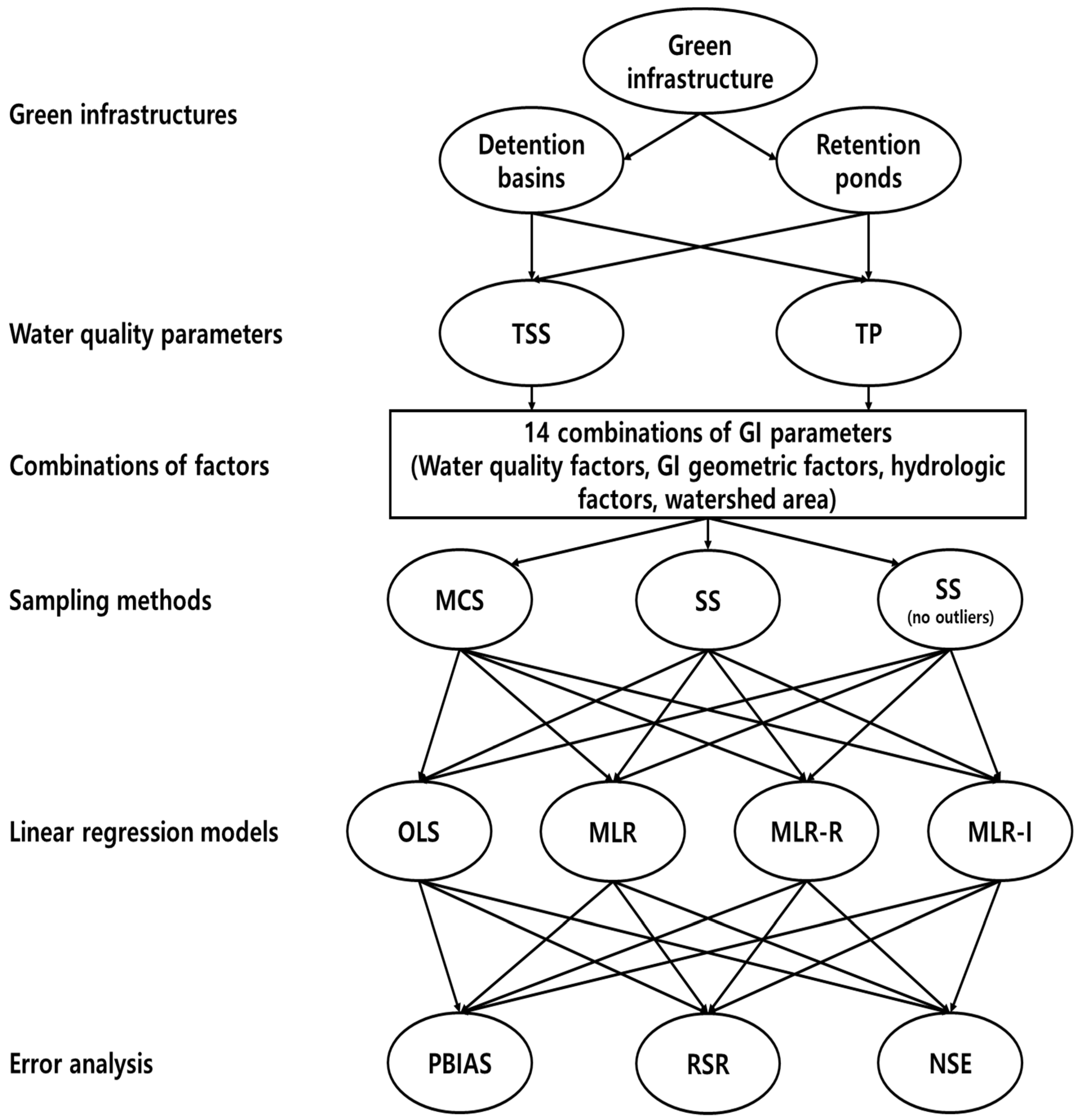
2. Methods
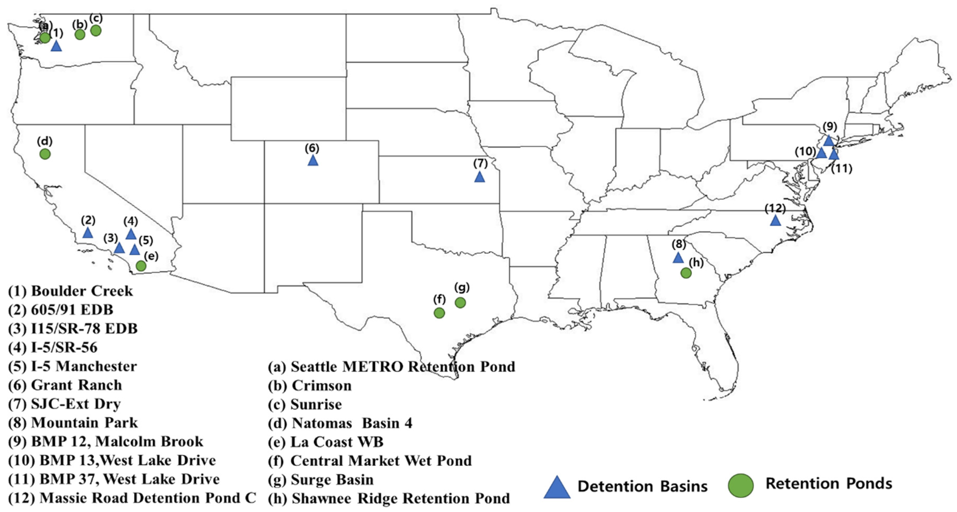
2.1. Stormwater BMP Database
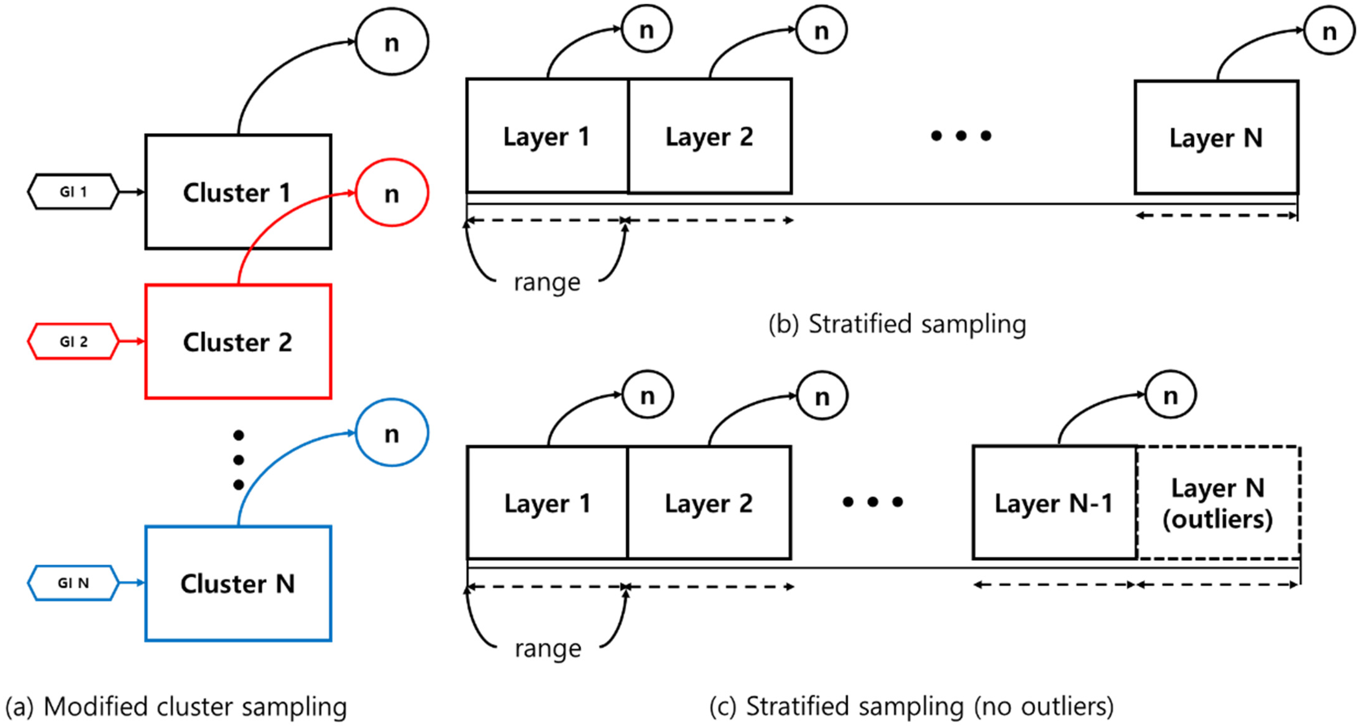
2.2. Sampling Methods
2.2.1. Modified Cluster Sampling (MCS)
2.2.2. Stratified Sampling
2.2.3. Stratified Sampling (No Outliers)
2.3. Linear Model Regression
2.3.1. OLS Regression
2.3.2. MLR
2.3.3. MLR-Interactions
2.3.4. MLR-Robust Fit
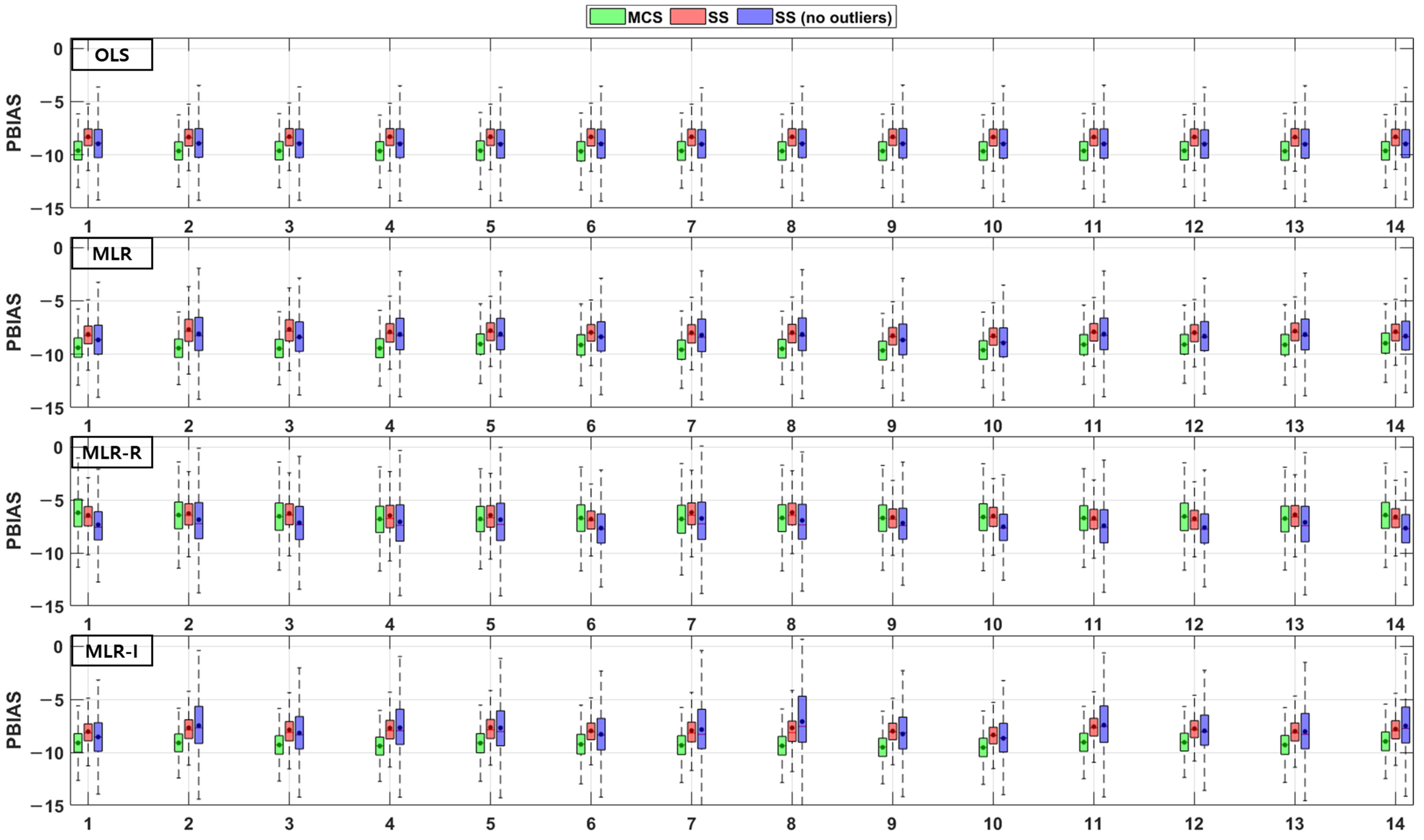
2.4. Model Evaluations (PBIAS, RSR, NSE)
2.4.1. Root Mean Square Error-Observations Standard Deviation Ratio (RSR)
2.4.2. Percent Bias (PBIAS)
2.4.3. Nash-Sutcliffe Efficiency (NSE)
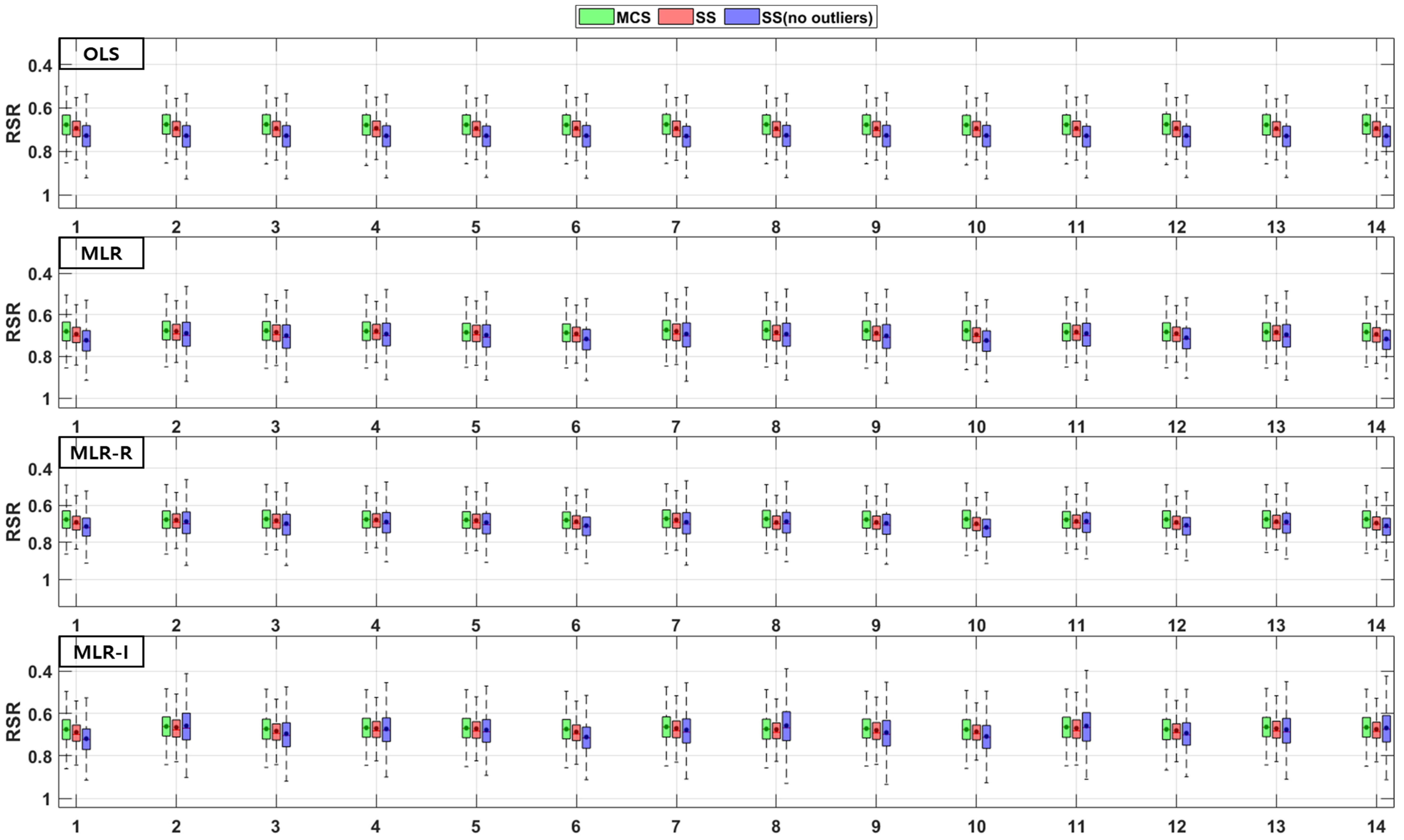
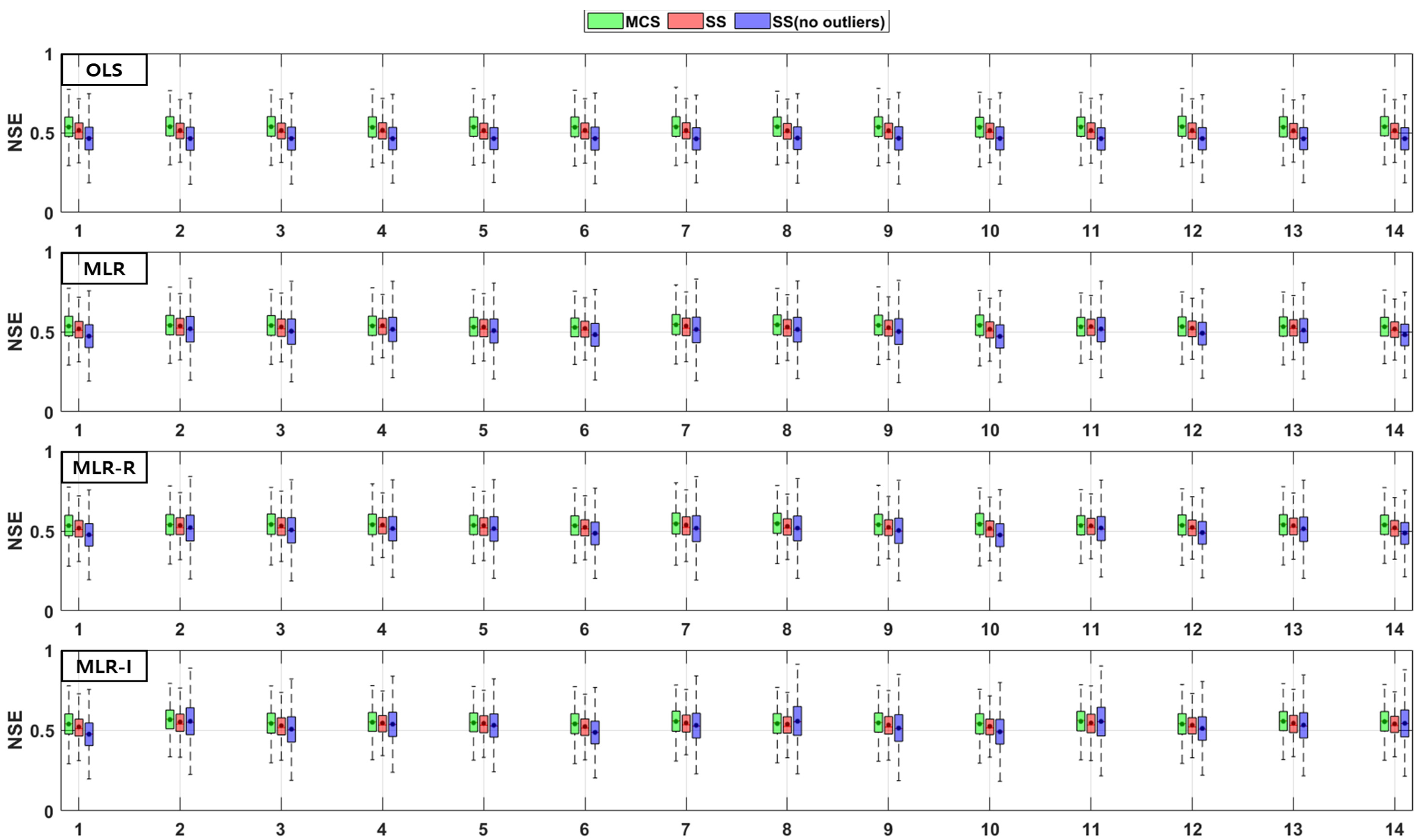
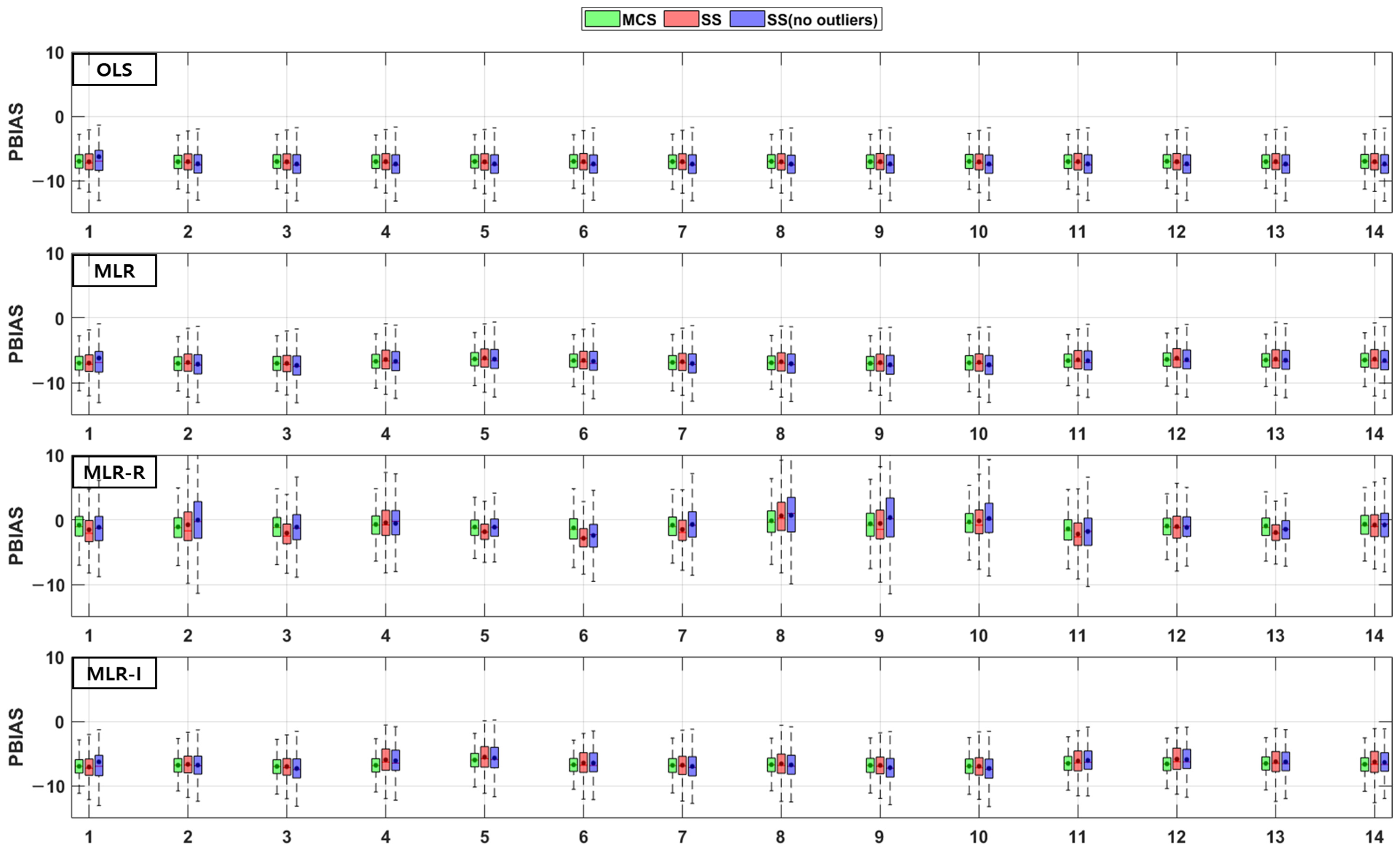
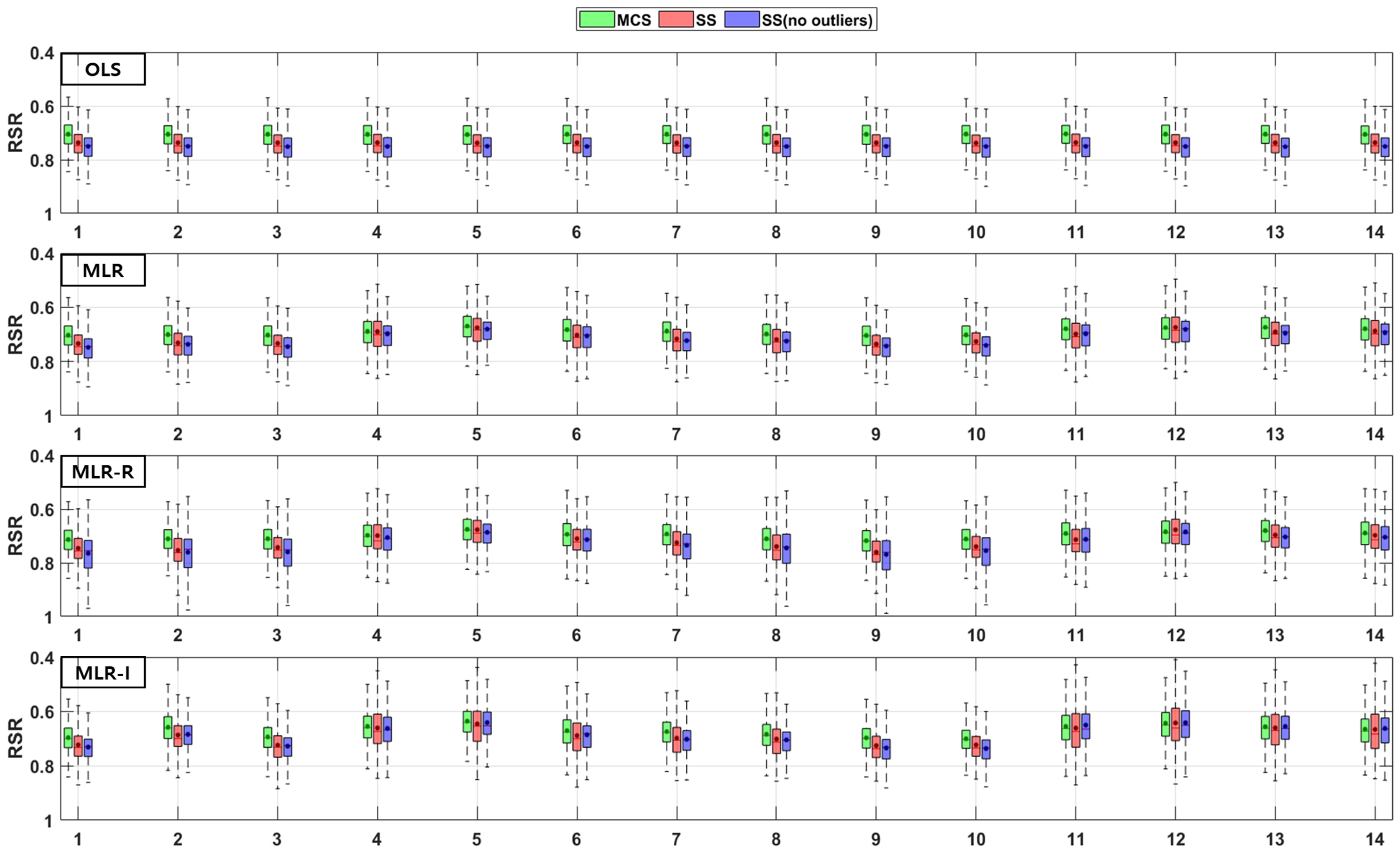
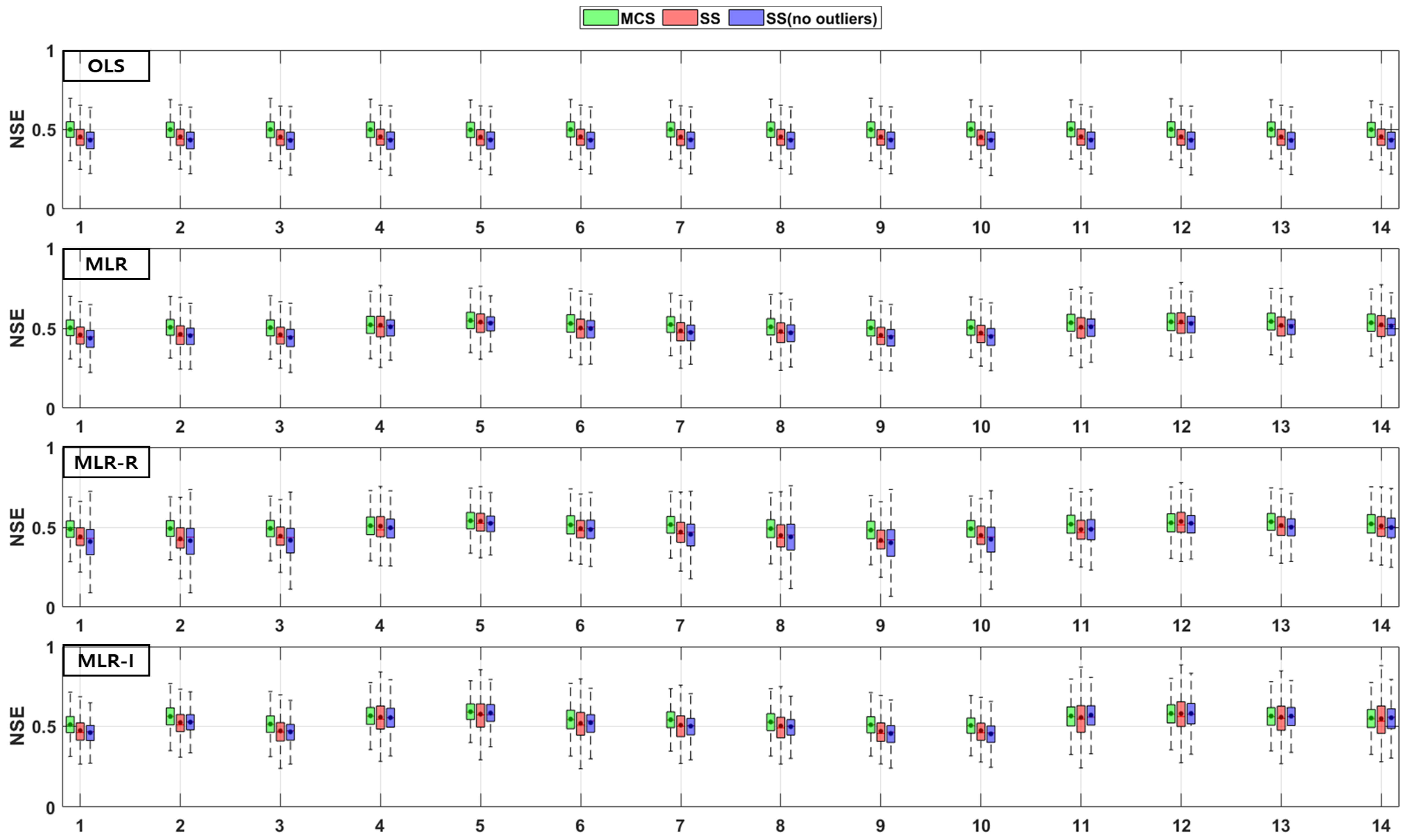
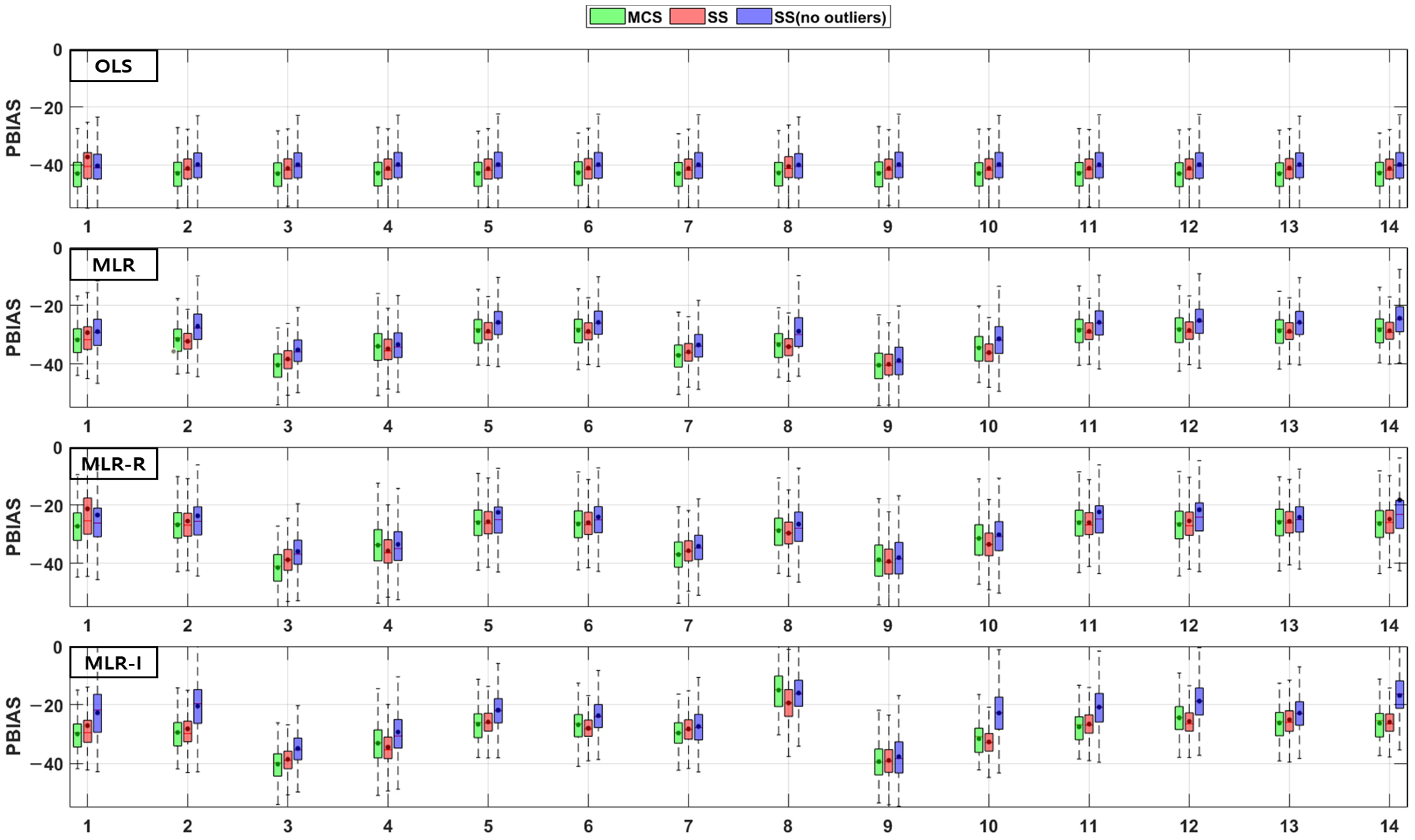
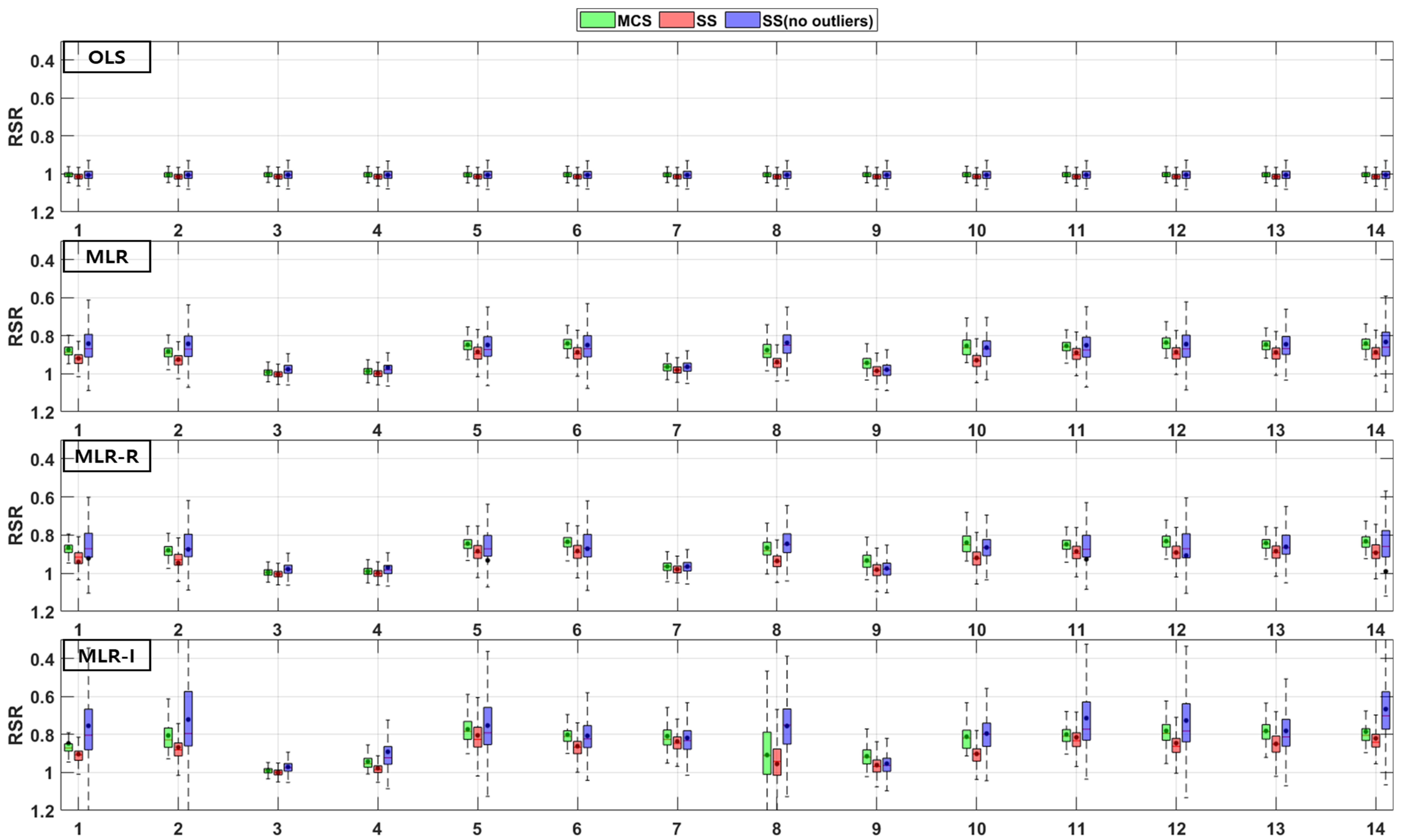
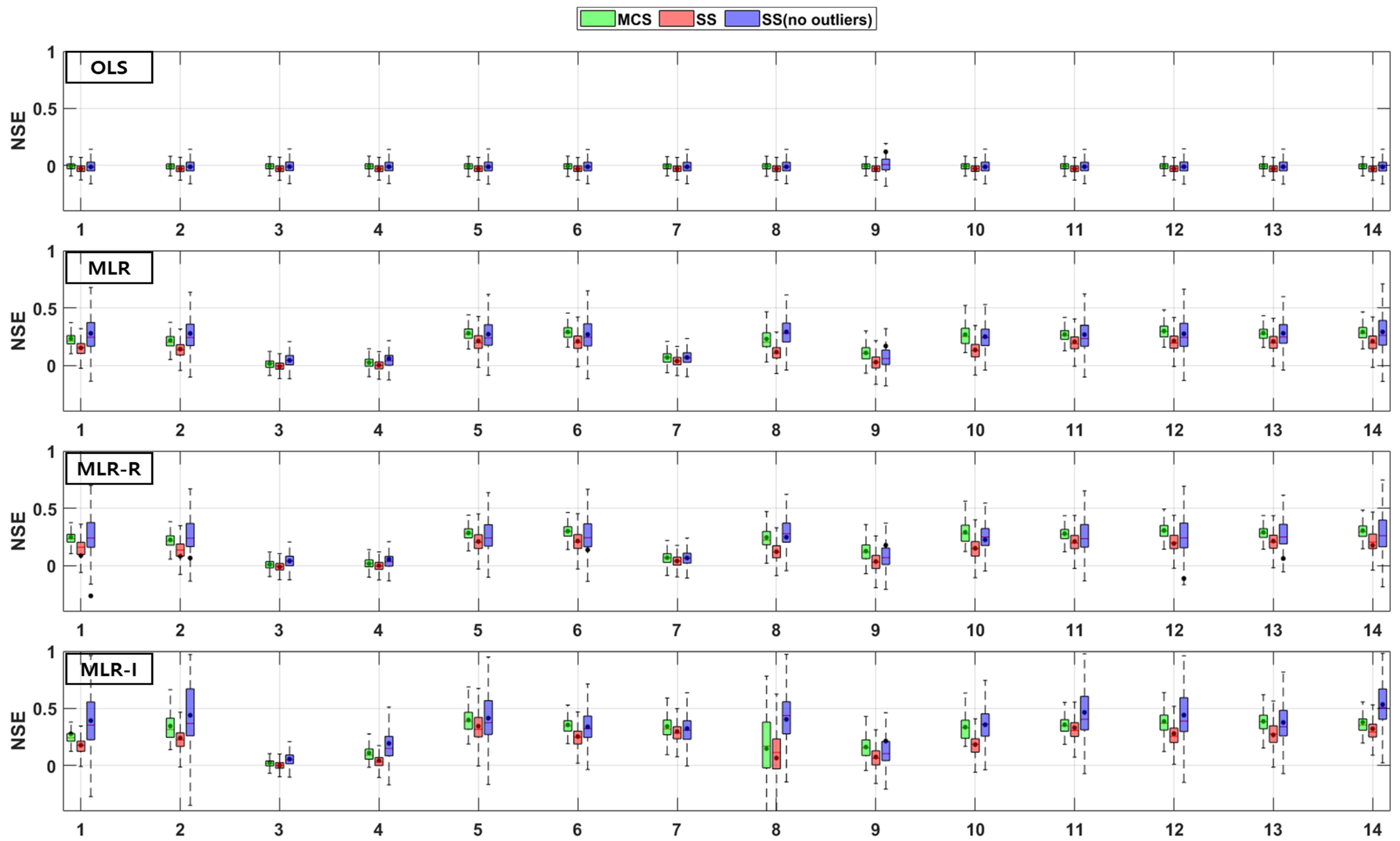
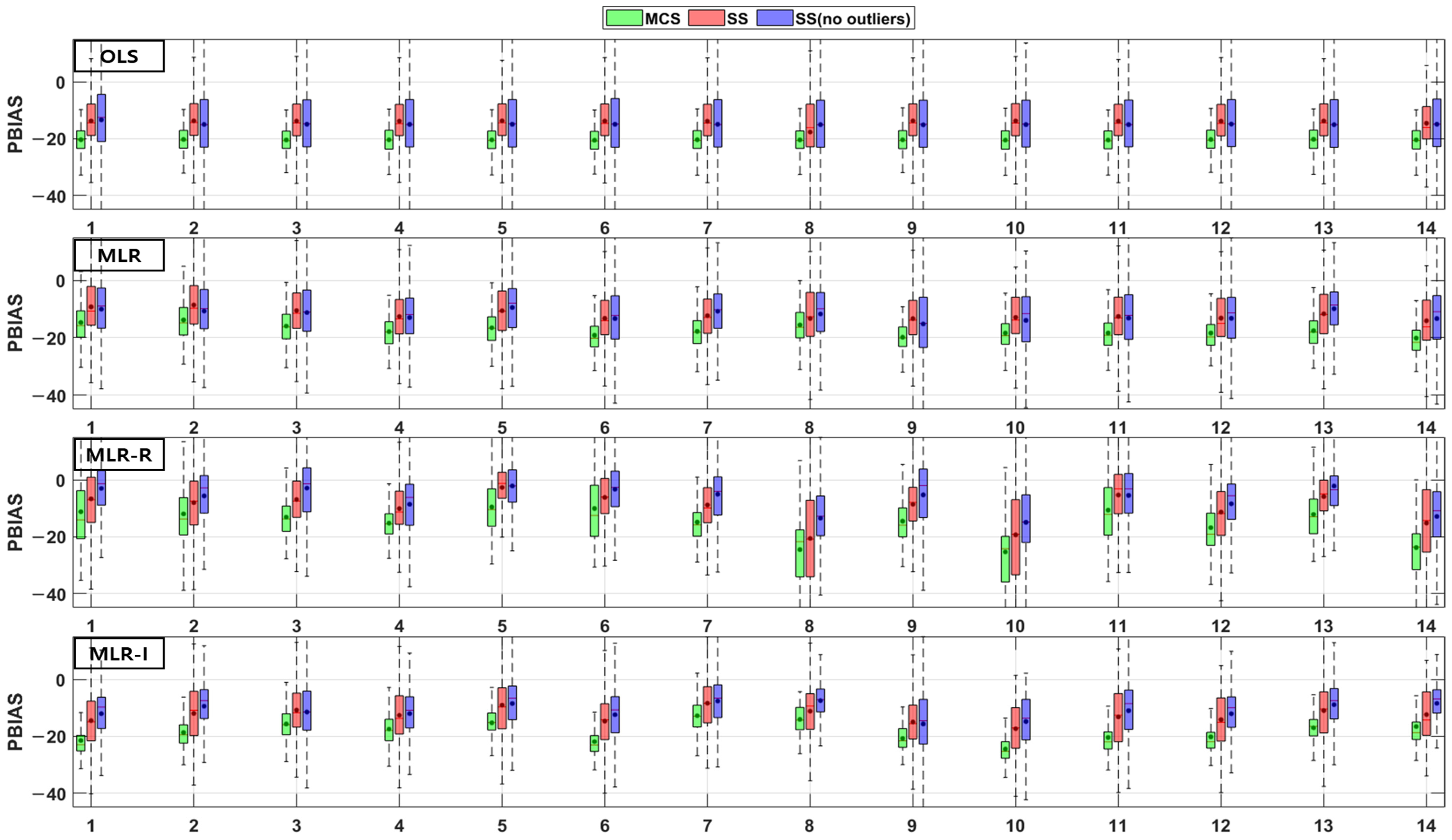
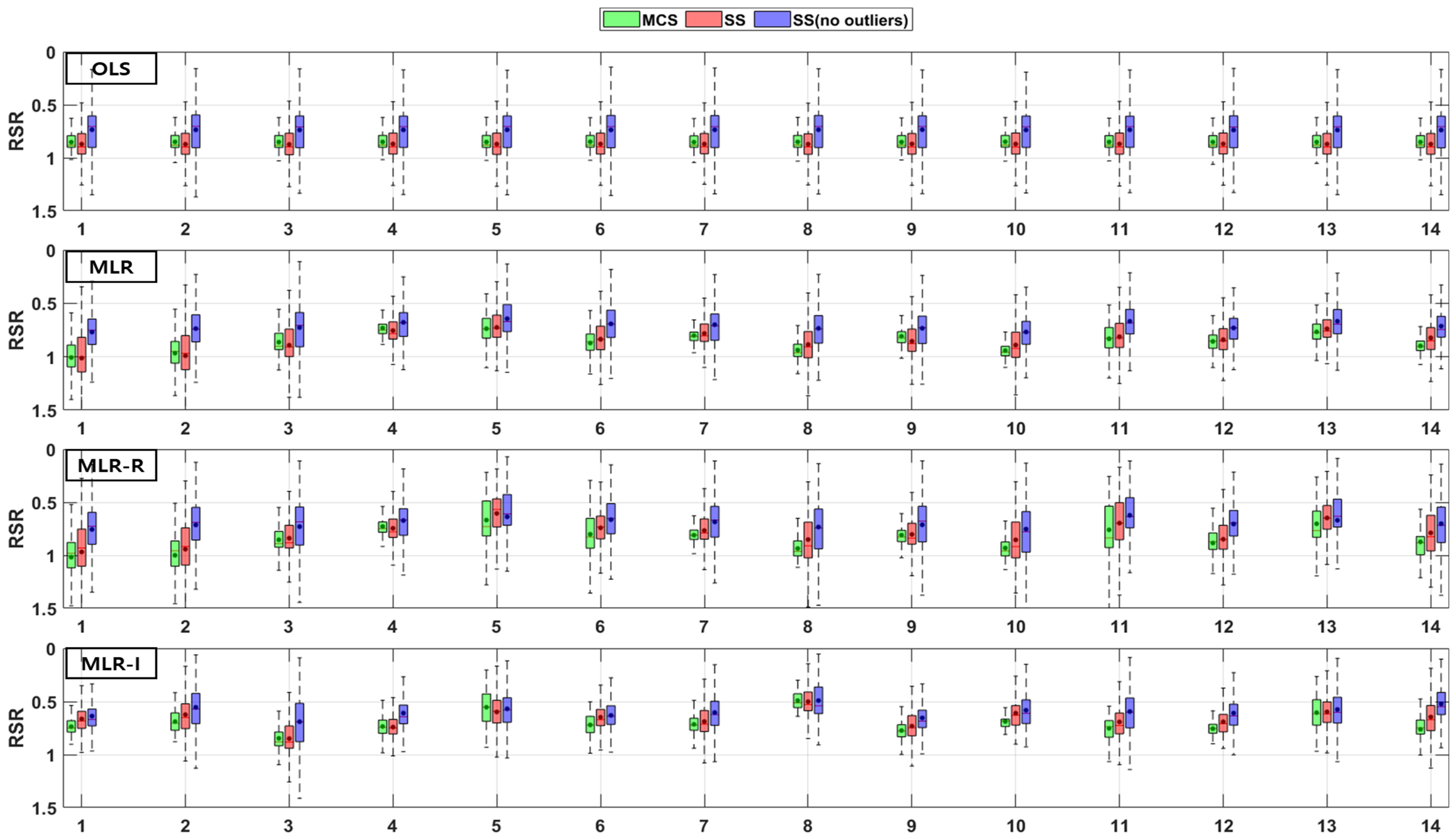
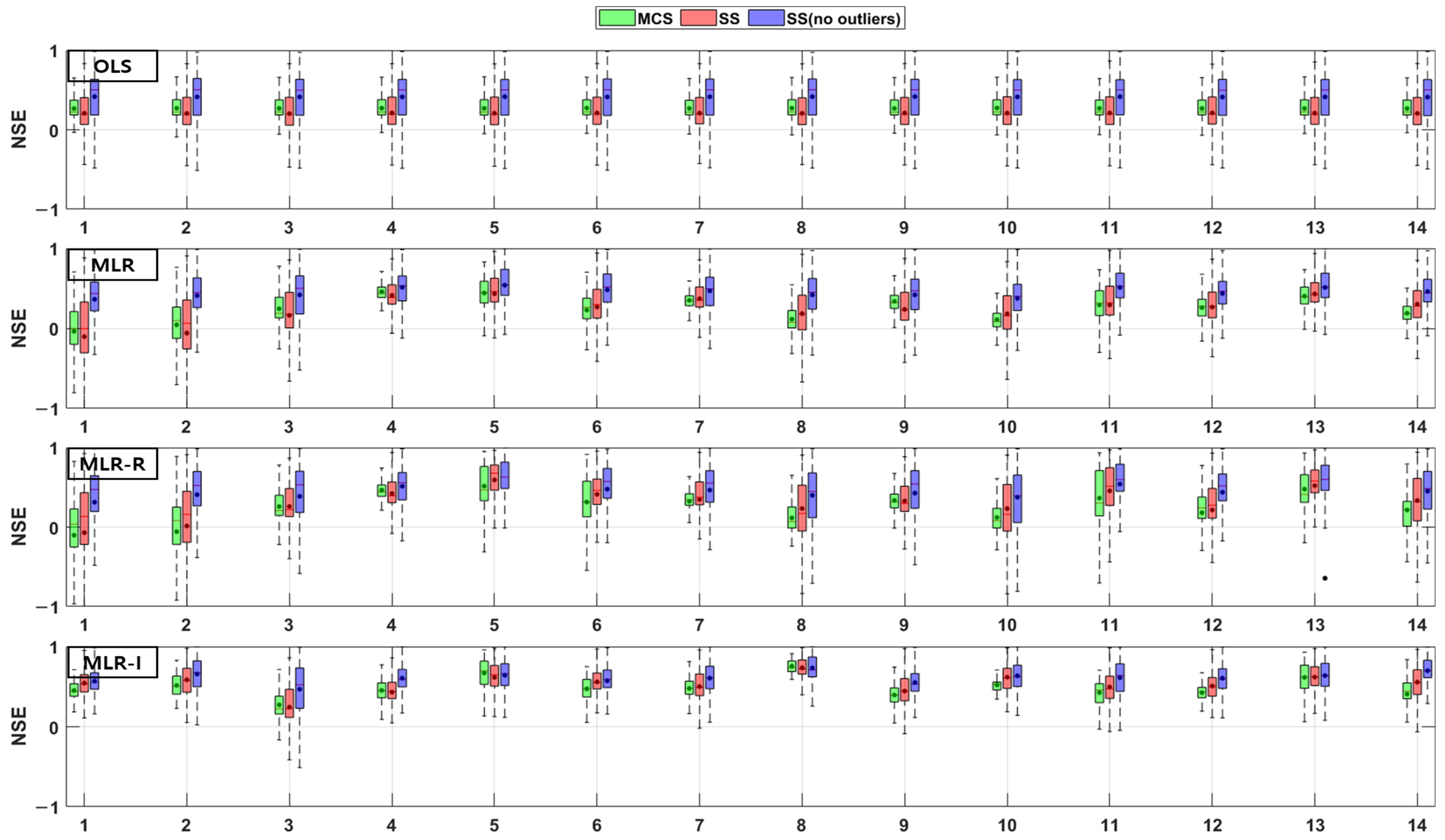
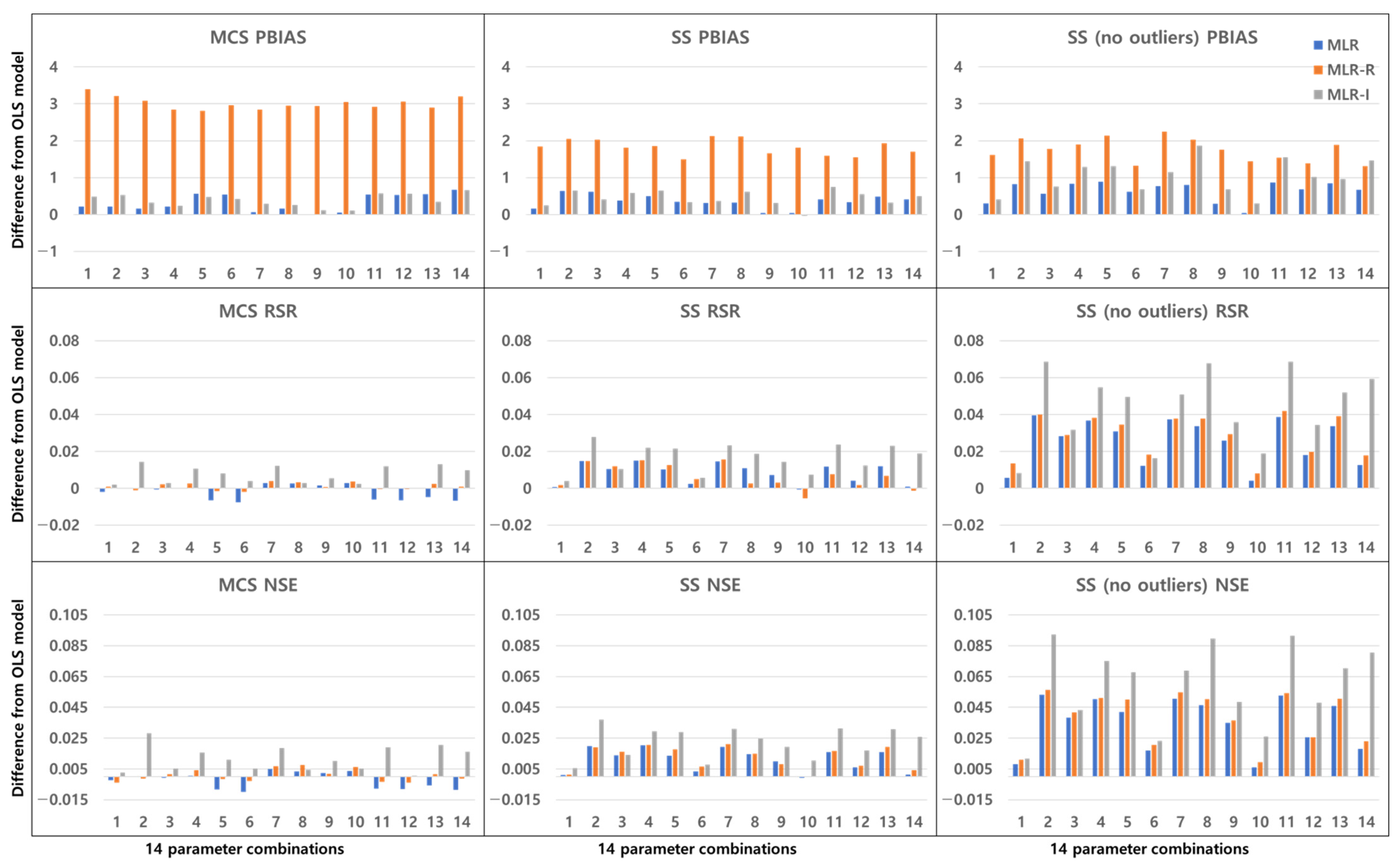
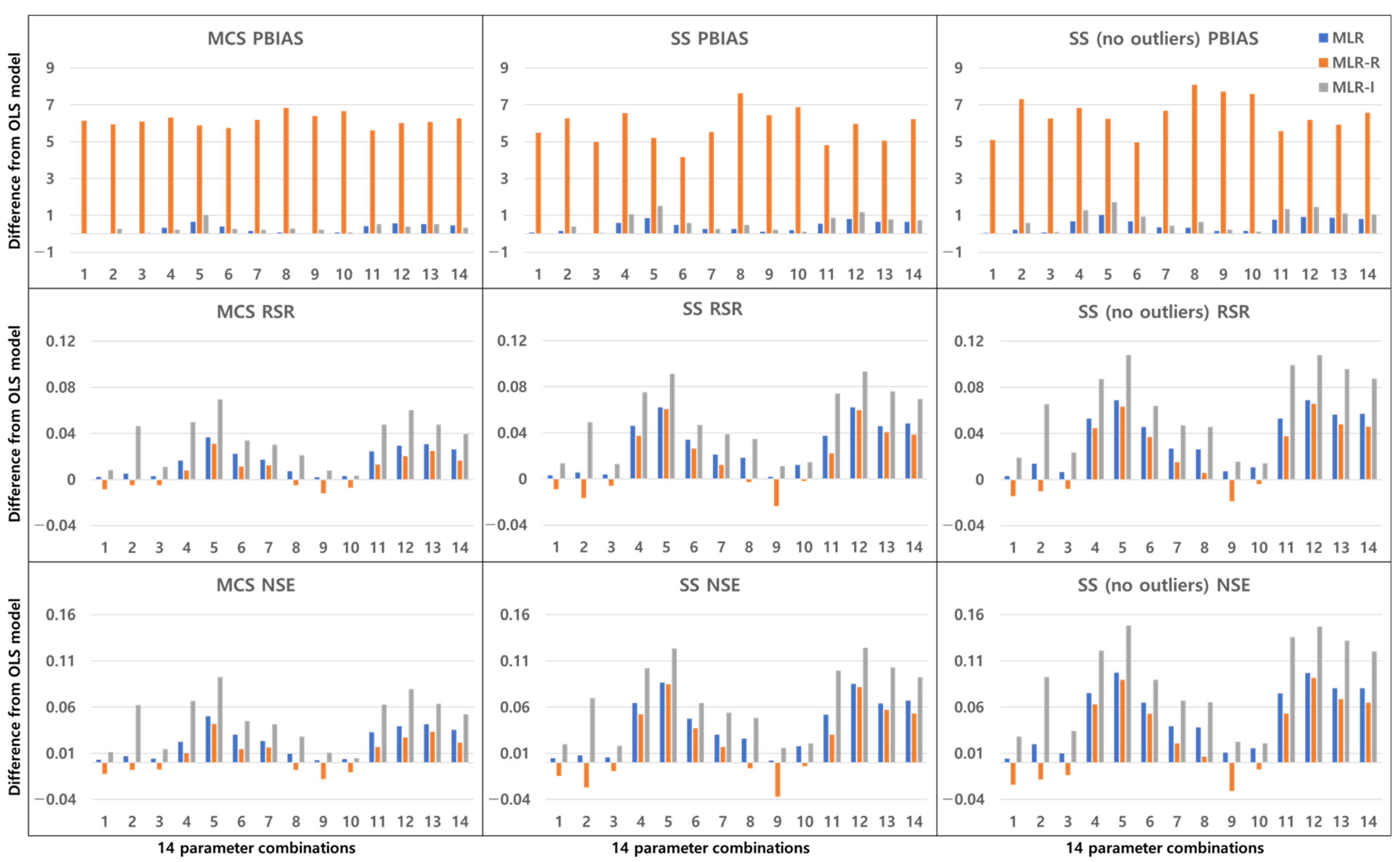
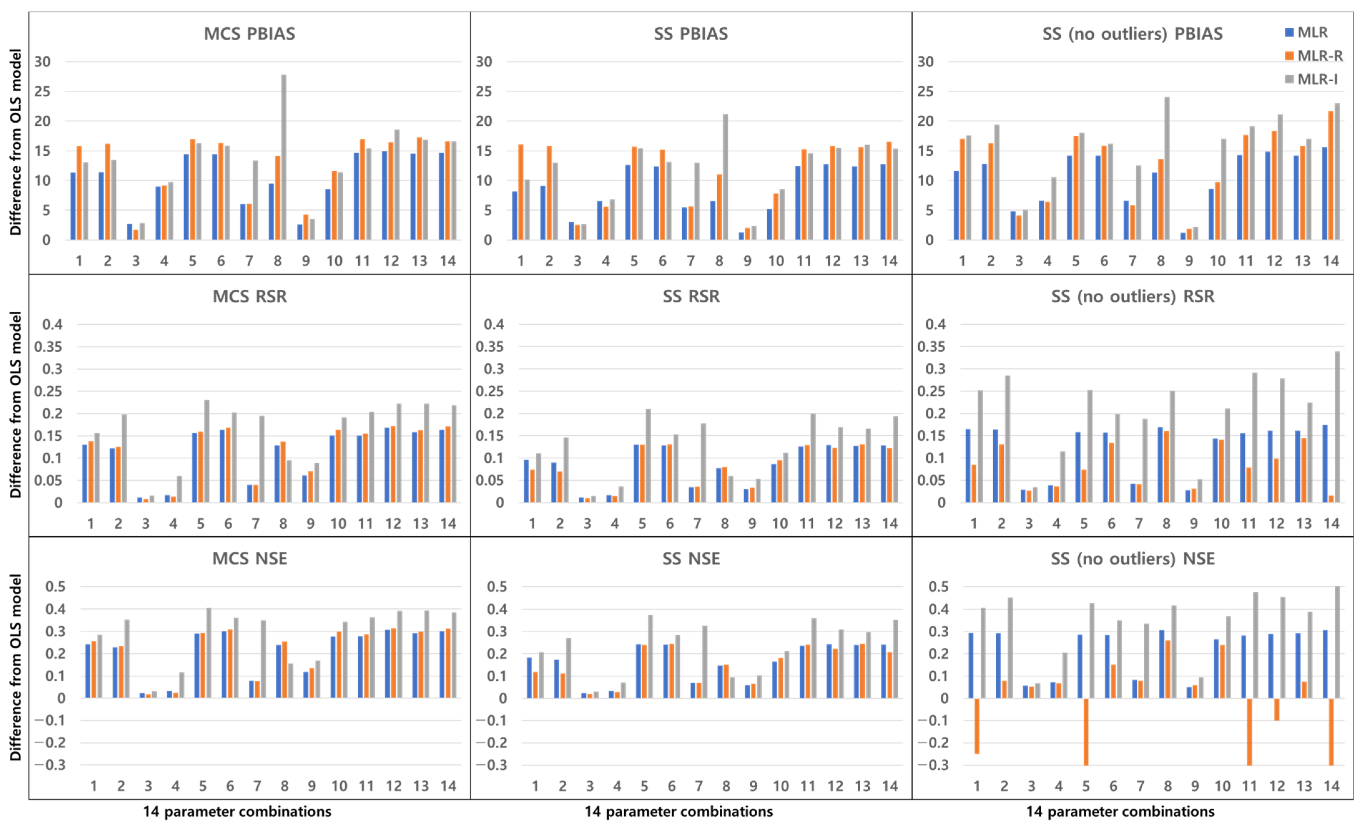
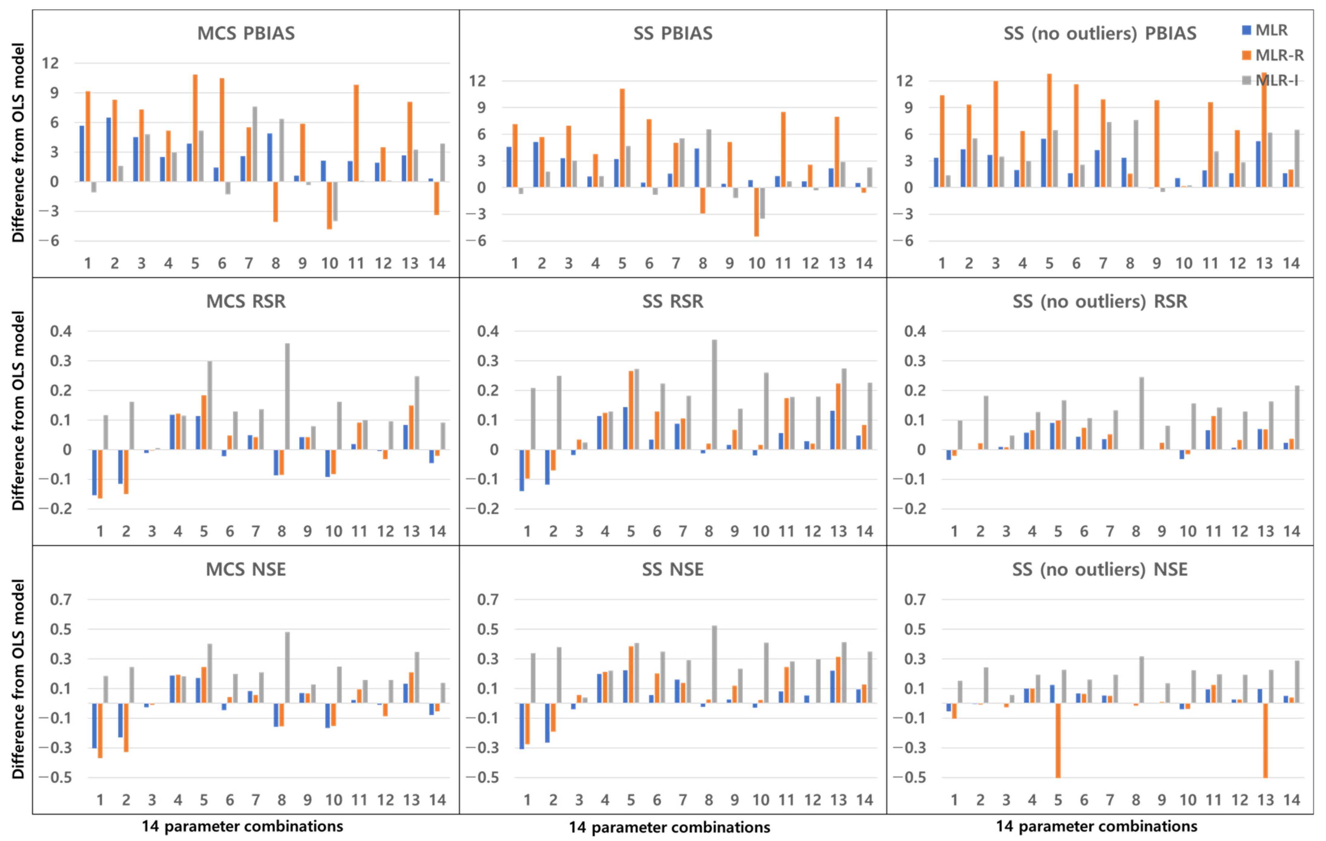
3. Results
3.1. GI Performance
3.2. Combinations of Parameters
4. Discussion
5. Conclusions
Author Contributions
Funding
Institutional Review Board Statement
Informed Consent Statement
Acknowledgments
Conflicts of Interest
References
- Yu, J.; Yu, H.; Xu, L. Performance Evaluation of Various Stormwater Best Management Practices. Environ. Sci Pollut Res. 2013, 20, 6160–6171. [Google Scholar] [CrossRef]
- Kadlec, R.H.; Knight, R.L. Treatment Wetlands; CRC Press: Boca Raton, FL, USA, 1996. [Google Scholar]
- Merriman, L.; Hathaway, J.; Burchell, M.; Hunt, W. Adapting the Relaxed Tanks-in-Series Model for Stormwater Wetland Water Quality Performance. Water 2017, 9, 691. [Google Scholar] [CrossRef] [Green Version]
- Barrett, M.E. Retention pond performance: Examples from the international stormwater BMP database. In Critical Transitions in Water and Environmental Resources Management; ASCE: Reston, VA, USA, 2004; pp. 1–10. [Google Scholar]
- United States Environmental Protection Agency (USEPA). Results of the Nationwide Urban. Runoff Program; R-554; United States Environmental Protection Agency (USEPA): Washington, DC, USA, 1983; Volume 1.
- Barrett, M.E. Comparison of BMP performance using the international BMP database. J. Irrig. Drain. Eng. 2008, 134, 556–561. [Google Scholar] [CrossRef]
- Strecker, E.W.; Quigley, M.M.; Urbonas, B.R.; Jones, J.E.; Clary, J.K. Determining Urban Storm Water BMP Effectiveness. J. Water Resour. Plan. Manag. 2001, 127, 144–149. [Google Scholar] [CrossRef]
- Barten, J.M. Stormwater Runoff Treatment in a Wetland Filter: Effects on the Water Quality of Clear Lake. Lake Reserv. Manag. 1987, 3, 297–305. [Google Scholar] [CrossRef]
- Hickok, E.A.; Hannaman, M.C.; Wenck, N.C. Urban Runoff Treatment Methods Volume I—Non-Structural Wetland Treatment; Office of Research and Development, Environmental Protection Agency: Washington, DC, USA, 1977.
- Meiorin, E.C. Urban runoff treatment in a fresh/brackish water marsh in Fremont, California. In Constructed Wetlands for Wastwater Treatment, Municipal, Industrial and Agricultural; Hammer, D.A., Ed.; Lewis Publishers: Chelsea, MI, USA, 1989; pp. 667–685. [Google Scholar]
- Scherger, D.A.; Davis, J.A. Control of stormwater runoff pollutant loads by a wetland and retention basin. In Proceedings of the International Symposium on Urban Hydrology, Hydraulics and Sediment Control, Lexington, KY, USA, 27–29 July 1982; pp. 109–123. [Google Scholar]
- Carleton, J.N.; Grizzard, T.J.; Godrej, A.N.; Post, H.E. Factors Affecting the Performance of Stormwater Treatment Wetlands. Water Res. 2001, 35, 1552–1562. [Google Scholar] [CrossRef]
- Strecker, E.W. The Use of Wetlands for Controlling Stormwater Pollution; Terrence Institute: Washington, DC, USA, 1992; p. 66. [Google Scholar]
- Shammaa, Y.; Zhu, D.Z.; Gyurek, L.L.; Labatiuk, C.W. Effectiveness of Dry Ponds for Stormwater Total Suspended Solids Removal. Can. J. Civ. Eng. 2002, 29, 316–324. [Google Scholar] [CrossRef]
- Papa, F.; Adams, B.J.; Guo, Y. Detention Time Selection for Stormwater Quality Control Ponds. Can. J. Civ. Eng. 1999, 26, 72–82. [Google Scholar] [CrossRef]
- Park, D.; Roesner, L.A. Effects of Surface Area and Inflow on the Performance of Stormwater Best Management Practices with Uncertainty Analysis. Water Environ. Res. 2013, 85, 782–792. [Google Scholar] [CrossRef]
- Gilliom, R.L.; Bell, C.D.; Hogue, T.S.; McCray, J.E. Adequacy of Linear Models for Estimating Stormwater Best Management Practice Treatment Performance. J. Sustain. Water Built Environ. 2020, 6, 4020016. [Google Scholar] [CrossRef]
- Etikan, I.; Bala, K. Sampling and sampling methods. Biom. Biostat. Int. J. 2017, 5, 215–217. [Google Scholar] [CrossRef] [Green Version]
- Hutcheson, G.D.; Moutinho, L. Ordinary Least-Squares Regression. In The SAGE Dictionary of Quantitative Management Research; SAGE Publications Ltd.: Thousand Oaks, CA, USA, 2011; pp. 224–228. [Google Scholar]
- Preacher, K.J.; Curran, P.J.; Bauer, D.J. Computational Tools for Probing Interactions in Multiple Linear Regression, Multilevel Modeling, and Latent Curve Analysis. J. Educ. Behav. Stat. 2006, 31, 437–448. [Google Scholar] [CrossRef]
- Holland, P.W.; Welsch, R.E. Robust Regression using Iteratively Reweighted Least-Squares. Communications in statistics. Theory Methods 1977, 6, 813–827. [Google Scholar] [CrossRef]
- Dumouchel, W.; O’Brien, F. Integrating a robust option into a multiple regression computing environment. In Computer Science and Statistics, Proceedings of the 21st Symposium on the Interface; American Statistical Association: Alexandria, VA, USA, 1989; pp. 297–302. [Google Scholar]
- Huber, P.J. Robust Statistics; Wiley: New York, NY, USA, 1981. [Google Scholar]
- Street, J.O.; Carroll, R.J.; Ruppert, D. A Note on Computing Robust Regression Estimates Via Iteratively Reweighted Least Squares. Am. Stat. 1988, 42, 152–154. [Google Scholar]
- Chu, T.; Shirmohammadi, A. Evaluation of the swat model’s hydrology component in the piedmont physiographic region of maryland. Trans. ASAE 2004, 47, 1057–1073. [Google Scholar] [CrossRef]
- Singh, J.; Knapp, H.V.; Arnold, J.G.; Demissie, M. Hydrological Modeling of the Iroquois River Watershed Using HSPF and SWAT1. J. Am. Water Resour. Assoc. 2005, 41, 343–360. [Google Scholar] [CrossRef]
- Vazquez-Amábile, G.G.; Engel, B.A. Use of SWAT to Compute Groundwater Table Depth and Streamflow in the Muscatatuck River Watershed. Trans. ASAE 2005, 48, 991–1003. [Google Scholar] [CrossRef] [Green Version]
- Moriasi, D.N.; Arnold, J.G.; Van Liew, M.W.; Bingner, R.L.; Harmel, R.D.; Veith, T.L. Model Evaluation Guidelines for Systematic Quantification of Accuracy in Watershed Simulations. Trans. ASABE 1983, 50, 885–900. [Google Scholar] [CrossRef]
- Gupta, H.V.; Sorooshian, S.; Yapo, P.O. Status of Automatic Calibration for Hydrologic Models: Comparison with Multilevel Expert Calibration. J. Hydrol. Eng. 1999, 4, 135–143. [Google Scholar] [CrossRef]
- Nash, J.E.; Suttcliffe, J.E. River Flow Forecasting Through Conceptual Models—Part I: A Discussion of Principles. J. Hydrol. 1970, 10, 282–290. [Google Scholar] [CrossRef]
- Urbonas, B.; Quigley, M.M.; Strecker, E.W. Results of Analyses of the Expanded EPA/ASCE National BMP Database. In Proceedings of the World Water & Environmental Resources Congress, Philadelphia, PA, USA, 23–26 June 2003; pp. 1–9. [Google Scholar]
- Walker, W.W. Phosphorus Removal by Urban Runoff Detention Basins. Lake Reserv. Manag. 1987, 3, 314–326. [Google Scholar] [CrossRef]


| GI | Area (m2) | Depth (m) | Volume (m3) | Watershed Area (km2) | FlowRate (m3/s) | Detention Time (s) | HLR (m/s) | Influent Concentration (Cin) (mg/L) | |
|---|---|---|---|---|---|---|---|---|---|
| Detention Basins | TSS | 800 | 0.4 | 200 | 20,000 | 0.001 | 20,000 | 2.0 × 10⁻⁶ | 30 |
| TP | 250 | 0.7 | 600 | 40,000 | 0.004 | 30,000 | 5.0 × 10⁻⁶ | 0.1 | |
| Retention Ponds | TSS | 1000 | 0.35 | 1000 | 100,000 | 0.01 | 20,000 | 1.0 × 10⁻⁶ | 50 |
| TP | 4000 | 0.4 | 2000 | 300,000 | 0.05 | 50,000 | 1.0 × 10⁻⁶ | 0.5 |
| Criteria | PBIAS | RSR | NSE |
|---|---|---|---|
| Good | −10% < PBIAS < 10% | RSR < 0.80 | NSE > 0.6 |
| Acceptable | −25% < PBIAS < 25% | 0.80 < RSR < 0.98 | 0.4 < NSE < 0.6 |
| Poor | PBIAS < −25%, PBIAS > 25% | RSR > 0.98 | NSE < 0.4 |
| Numbers | 1 | 2 | 3 | 4 | 5 | 6 | 7 | 8 | 9 | 10 | 11 | 12 | 13 | 14 |
|---|---|---|---|---|---|---|---|---|---|---|---|---|---|---|
| Combinations | Cin, HLR | Cin, Q, A | Cin, Q | Cin, Q, D | Cin, Q, V | Cin, T | Cin, Q, WA | Cin, Q, A/WA | Cin, A | Cin, A/WA | Cin, T, A | Cin, T, D | Cin, T, WA | Cin, T, A/WA |
Publisher’s Note: MDPI stays neutral with regard to jurisdictional claims in published maps and institutional affiliations. |
© 2021 by the authors. Licensee MDPI, Basel, Switzerland. This article is an open access article distributed under the terms and conditions of the Creative Commons Attribution (CC BY) license (https://creativecommons.org/licenses/by/4.0/).
Share and Cite
Jeon, S.; Kim, S.; Lee, M.; An, H.; Jung, K.; Um, M.-J.; An, K.; Park, D. Insights into the Pollutant Removal Performance of Stormwater Green Infrastructures: A Case Study of Detention Basins and Retention Ponds. Int. J. Environ. Res. Public Health 2021, 18, 10104. https://0-doi-org.brum.beds.ac.uk/10.3390/ijerph181910104
Jeon S, Kim S, Lee M, An H, Jung K, Um M-J, An K, Park D. Insights into the Pollutant Removal Performance of Stormwater Green Infrastructures: A Case Study of Detention Basins and Retention Ponds. International Journal of Environmental Research and Public Health. 2021; 18(19):10104. https://0-doi-org.brum.beds.ac.uk/10.3390/ijerph181910104
Chicago/Turabian StyleJeon, Seol, Siyeon Kim, Moonyoung Lee, Heejin An, Kichul Jung, Myoung-Jin Um, Kyungjin An, and Daeryong Park. 2021. "Insights into the Pollutant Removal Performance of Stormwater Green Infrastructures: A Case Study of Detention Basins and Retention Ponds" International Journal of Environmental Research and Public Health 18, no. 19: 10104. https://0-doi-org.brum.beds.ac.uk/10.3390/ijerph181910104