Identification Framework of Contaminant Spill in Rivers Using Machine Learning with Breakthrough Curve Analysis


Abstract
:1. Introduction
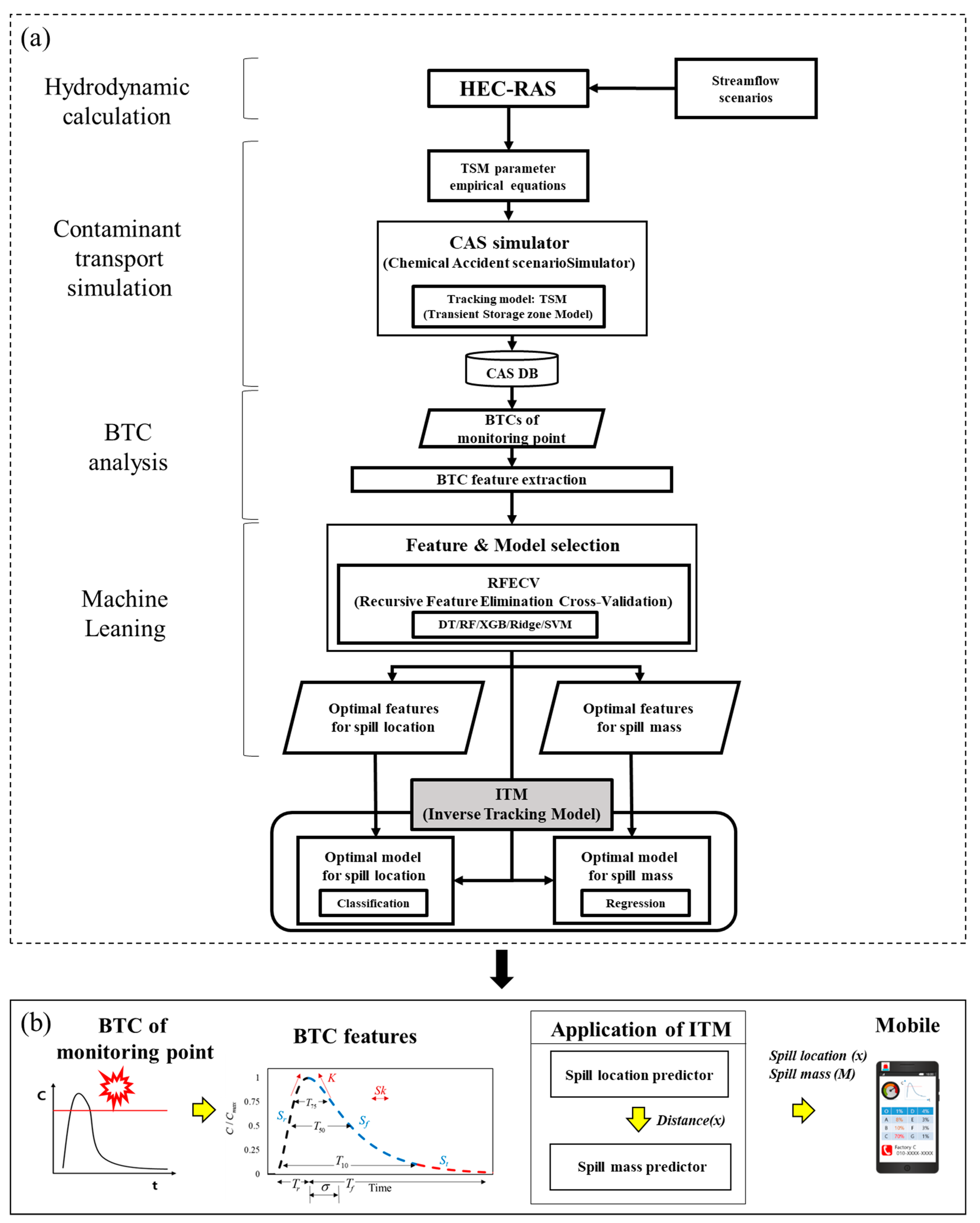
2. Methodology
2.1. Contaminant Accident Scenarios (CAS)
2.1.1. Transient Storage Model (TSM)
2.1.2. CAS Simulation
2.2. Breakthrough Curve (BTC) Analysis
2.3. Machine Learning (ML) Modeling
2.3.1. DT-Based Models
2.3.2. SVM and Ridge Regression
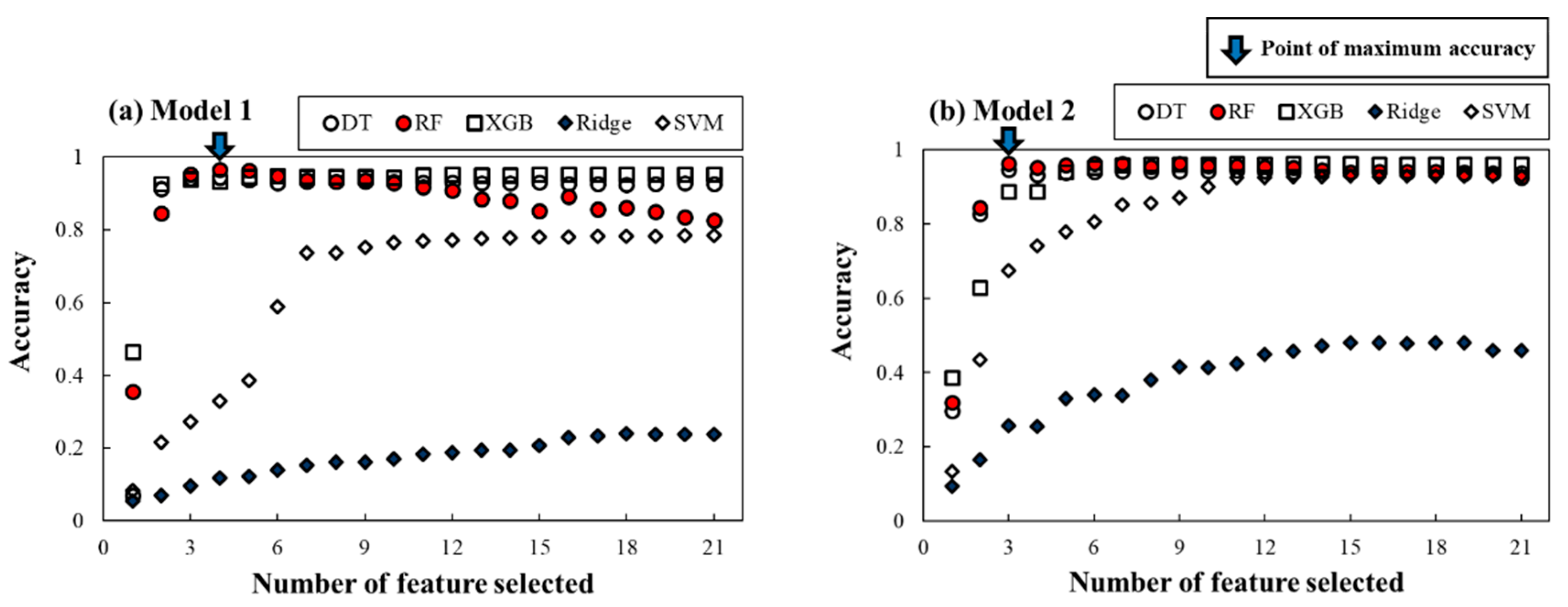
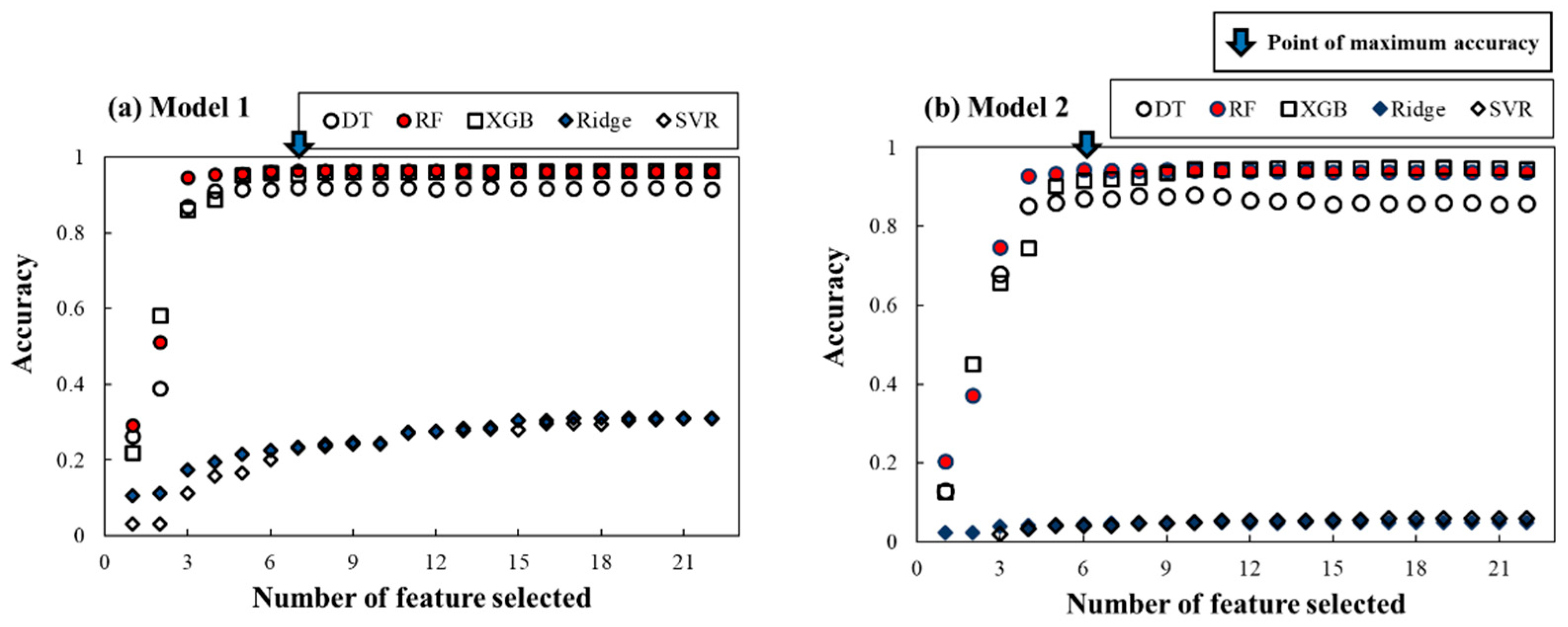
2.4. Feature Importance and Feature Selection
2.5. Modeling Performance Criteria
3. Study Site and Field Tracer Test
4. Development of the ITM Framework in Gam Creek
4.1. Chemical Accident Scenarios in Gam Creek
4.2. Model Development
4.2.1. BTC Feature Importance for Inverse Tracking the Contaminant Source
4.2.2. Development of Spill Location Predictor
4.2.3. Development of Spill Mass Predictor
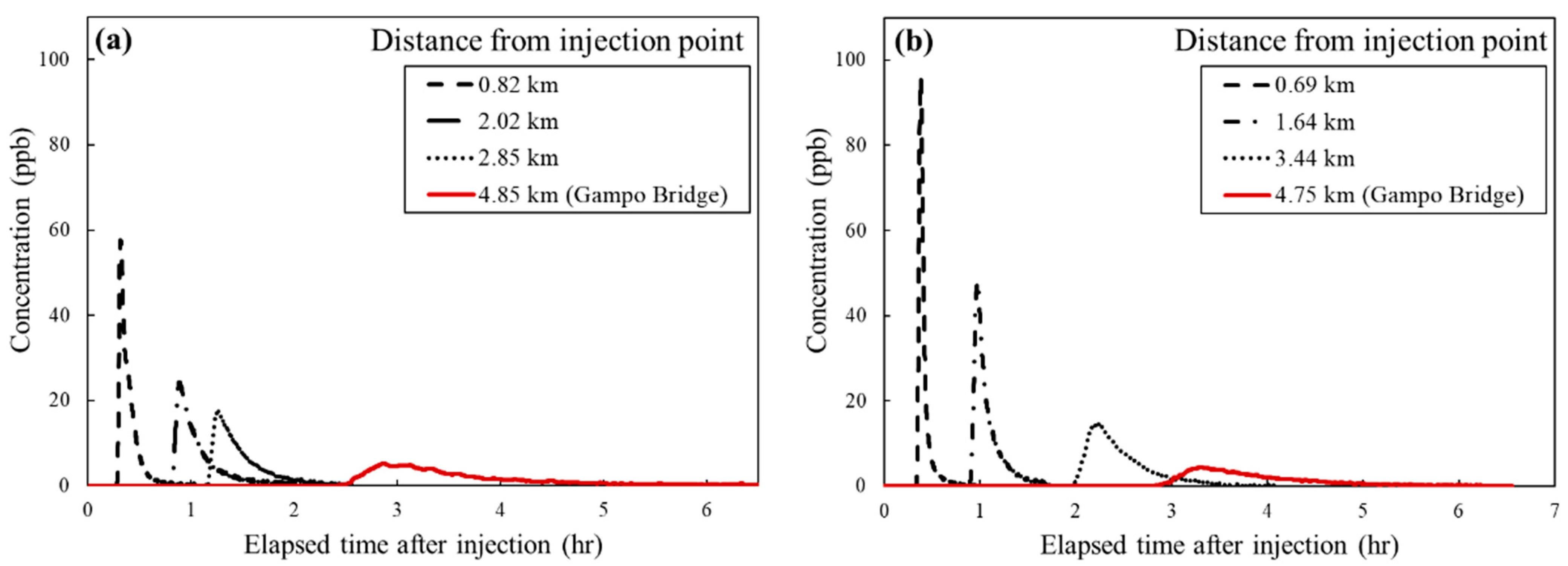
5. Field Application of ITM
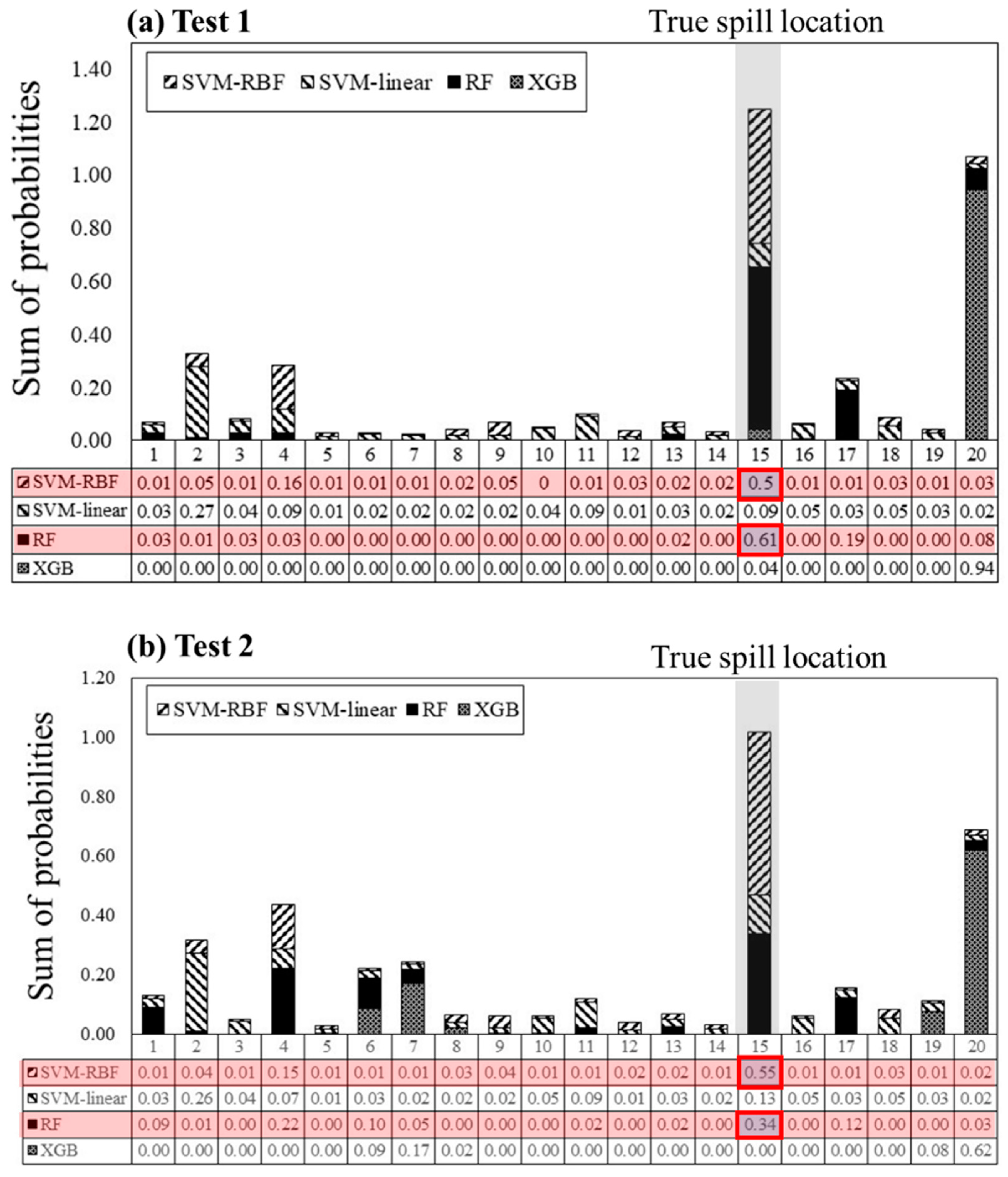
5.1. Field Test of Spill Location Predictors
5.2. Field Test of Spill Mass Predictors
6. Conclusions
Author Contributions
Funding
Institutional Review Board Statement
Informed Consent Statement
Acknowledgments
Conflicts of Interest
References
- Guozhen, W.; Zhang, C.; Li, Y.; Haixing, L.; Zhou, H. Source identification of sudden contamination based on the parameter uncertainty analysis. J. Hydroinform. 2016, 18, 919–927. [Google Scholar] [CrossRef]
- Wang, J.; Zhao, J.; Lei, X.; Wang, H. An effective method for point pollution source identification in rivers with performance-improved ensemble Kalman filter. J. Hydrol. 2019, 577, 123991. [Google Scholar] [CrossRef]
- Yang, H.; Shao, D.; Liu, B.; Huang, J.; Ye, X. Multi-point source identification of sudden water pollution accidents in surface waters based on differential evolution and Metropolis–Hastings–Markov Chain Monte Carlo. Stoch. Environ. Res. Risk Assess. 2015, 30, 507–522. [Google Scholar] [CrossRef]
- Singh, P.; Singh, R.M. Identification of pollution sources using artificial neural network (ANN) and multilevel breakthrough curve (BTC) characterization. Environ. Forensics 2019, 20, 219–227. [Google Scholar] [CrossRef]
- Franssen, H.H.; Alcolea, A.; Riva, M.; Bakr, M.; Van Der Wiel, N.; Stauffer, F.; Guadagnini, A. A comparison of seven methods for the inverse modelling of groundwater flow. Application to the characterisation of well catchments. Adv. Water Res. 2009, 32, 851–872. [Google Scholar] [CrossRef]
- Srivastava, D.; Singh, R.M. Breakthrough Curves Characterization and Identification of an Unknown Pollution Source in Groundwater System Using an Artificial Neural Network (ANN). Environ. Forensics 2014, 15, 175–189. [Google Scholar] [CrossRef]
- Atmadja, J.; Bagtzoglou, A. State of the Art Report on Mathematical Methods for Groundwater Pollution Source Identification. Environ. Forensics 2001, 2, 205–214. [Google Scholar] [CrossRef]
- Vesselinov, V.V.; Alexandrov, B.S.; O’Malley, D. Contaminant source identification using semi-supervised machine learning. J. Contam. Hydrol. 2018, 212, 134–142. [Google Scholar] [CrossRef]
- Vesselinov, V.V.; Alexandrov, B.S.; O’Malley, D. Nonnegative tensor factorization for contaminant source identification. J. Contam. Hydrol. 2019, 220, 66–97. [Google Scholar] [CrossRef]
- Wallis, S.G.; Bonardi, D.; Silavwe, D. Solute transport routing in a small stream. Hydrol. Sci. J. 2014, 59, 1894–1907. [Google Scholar] [CrossRef]
- Singh, R.M.; Datta, B. Identification of groundwater pollution sources using GA-based linked simulation optimization model. J. Hydrol. Eng. 2006, 11, 631–635. [Google Scholar] [CrossRef]
- Srivastava, D.; Singh, R.M. Groundwater System Modeling for Simultaneous Identification of Pollution Sources and Parameters with Uncertainty Characterization. Water Res. Manag. 2015, 29, 4607–4627. [Google Scholar] [CrossRef]
- Chen, Z.; Gómez-Hernández, J.J.; Zanini, A.; Gómez-Hernández, J.J. Joint identification of contaminant source and aquifer geometry in a sandbox experiment with the restart ensemble Kalman filter. J. Hydrol. 2018, 564, 1074–1084. [Google Scholar] [CrossRef]
- Cabral-Pinto, M.M.; Inácio, M.; Neves, O.; Almeida, A.A.; Pinto, E.; Oliveiros, B.; Da Silva, E.A.F. Human Health Risk Assessment Due to Agricultural Activities and Crop Consumption in the Surroundings of an Industrial Area. Expo. Health 2020, 12, 629–640. [Google Scholar] [CrossRef]
- Cabral-Pinto, M.M.; Reis, P.M.; Almeida, A.; Pinto, E.; Neves, M.O.; Inácio, M.; Gerardo, B.; Freitas, S.; Simões, M.R.; Dinis, P.A.; et al. Links between Cognitive Status and Trace Element Levels in Hair for an Environmentally Exposed Population: A Case Study in the Surroundings of the Estarreja Industrial Area. Int. J. Environ. Res. Public Health 2019, 16, 4560. [Google Scholar] [CrossRef] [PubMed] [Green Version]
- Parolin, R.D.S.; Neto, A.J.S.; Rodrigues, P.; Llanes-Santiago, O. Estimation of a contaminant source in an estuary with an inverse problem approach. Appl. Math. Comput. 2015, 260, 331–341. [Google Scholar] [CrossRef]
- Zhang, S.-P.; Xin, X.-K. Pollutant source identification model for water pollution incidents in small straight rivers based on genetic algorithm. Appl. Water Sci. 2016, 7, 1955–1963. [Google Scholar] [CrossRef] [Green Version]
- Jiang, J.; Han, F.; Zheng, Y.; Wang, N.; Yuan, Y. Inverse uncertainty characteristics of pollution source identification for river chemical spill incidents by stochastic analysis. Front. Environ. Sci. Eng. 2018, 12, 6. [Google Scholar] [CrossRef]
- Cheng, W.; Jia, Y. Identification of contaminant point source in surface waters based on backward location probability density function method. Adv. Water Res. 2010, 33, 397–410. [Google Scholar] [CrossRef]
- Ghane, A.; Mazaheri, M.; Samani, J.M.V. Location and release time identification of pollution point source in river networks based on the Backward Probability Method. J. Environ. Manag. 2016, 180, 164–171. [Google Scholar] [CrossRef]
- Boano, F.; Revelli, R.; Ridolfi, L. Source identification in river pollution problems: A geostatistical approach. Water Resour. Res. 2005, 41, 1–13. [Google Scholar] [CrossRef]
- Hazart, A.; Giovannelli, J.-F.; Dubost, S.; Chatellier, L. Inverse transport problem of estimating point-like source using a Bayesian parametric method with MCMC. Signal Process. 2014, 96, 346–361. [Google Scholar] [CrossRef]
- Telci, I.T.; Aral, M.M. Contaminant Source Location Identification in River Networks Using Water Quality Monitoring Systems for Exposure Analysis. Water Qual. Expo. Health 2011, 2, 205–218. [Google Scholar] [CrossRef]
- Kim, J.H.; Lee, M.L.; Park, C. A Data-Based Framework for Identifying a Source Location of a Contaminant Spill in a River System with Random Measurement Errors. Sensors 2019, 19, 3378. [Google Scholar] [CrossRef] [Green Version]
- Lee, Y.J.; Park, C.; Lee, M.L. Identification of a Contaminant Source Location in a River System Using Random Forest Models. Water 2018, 10, 391. [Google Scholar] [CrossRef] [Green Version]
- Liang, J.; Li, W.; Bradford, S.A.; Šimůnek, J. Physics-Informed Data-Driven Models to Predict Surface Runoff Water Quantity and Quality in Agricultural Fields. Water 2019, 11, 200. [Google Scholar] [CrossRef] [Green Version]
- Choi, S.Y.; Seo, I.W. Prediction of fecal coliform using logistic regression and tree-based classification models in the North Han River, South Korea. HydroResearch 2018, 21, 96–108. [Google Scholar] [CrossRef]
- Tyralis, H.; Papacharalampous, G.; Langousis, A. A Brief Review of Random Forests for Water Scientists and Practitioners and Their Recent History in Water Resources. Water 2019, 11, 910. [Google Scholar] [CrossRef] [Green Version]
- Choubin, B.; Darabi, H.; Rahmati, O.; Sajedi-Hosseini, F.; Kløve, B. River suspended sediment modelling using the CART model: A comparative study of machine learning techniques. Sci. Total. Environ. 2018, 615, 272–281. [Google Scholar] [CrossRef]
- Raghavendra, S.N.; Deka, P.C. Support vector machine applications in the field of hydrology: A review. Appl. Soft Comput. 2014, 19, 372–386. [Google Scholar] [CrossRef]
- Solomatine, D.P.; Ostfeld, A. Data-driven modelling: Some past experiences and new approaches. J. Hydroinform. 2008, 10, 3–22. [Google Scholar] [CrossRef] [Green Version]
- Yaseen, Z.M.; Sulaiman, S.O.; Deo, R.C.; Ahmadi, M.H. An enhanced extreme learning machine model for river flow forecasting: State-of-the-art, practical applications in water resource engineering area and future research direction. J. Hydrol. 2019, 569, 387–408. [Google Scholar] [CrossRef]
- Noori, R.; Deng, Z.; Kiaghadi, A.; Kachoosangi, F.T. How Reliable Are ANN, ANFIS, and SVM Techniques for Predicting Longitudinal Dispersion Coefficient in Natural Rivers? J. Hydraul. Eng. 2016, 142. [Google Scholar] [CrossRef]
- Gülbaz, S. Water quality model for nonpoint source pollutants incorporating bioretention with EPA SWMM. Desalination Water Treat. 2019, 164, 111–120. [Google Scholar] [CrossRef]
- Bencala, K.E.; Walters, R.A. Simulation of solute transport in a mountain pool-and-riffle stream: A transient storage model. Water Resour. Res. 1983, 19, 718–724. [Google Scholar] [CrossRef]
- Moghaddam, M.B.; Mazaheri, M.; Samani, J.M. A comprehensive one-dimensional numerical model for solute transport in rivers. Hydrol. Earth Syst. Sci. 2017, 21, 99–116. [Google Scholar] [CrossRef] [Green Version]
- Runkel, R.L. One-Dimensional Transport with Inflow and Storage (OTIS): A Solute Transport Model for Streams and Rivers; US Geological Survey: Reston, VA, USA, 1998; pp. 98–4018.
- Choi, S.Y.; Seo, I.W.; Kim, Y.-O. Parameter uncertainty estimation of transient storage model using Bayesian inference with formal likelihood based on breakthrough curve segmentation. Environ. Model. Softw. 2020, 123, 104558. [Google Scholar] [CrossRef]
- Noh, H.; Kwon, S.; Seo, I.W.; Baek, D.; Jung, S.H. Multi-Gene Genetic Programming Regression Model for Prediction of Transient Storage Model Parameters in Natural Rivers. Water 2020, 13, 76. [Google Scholar] [CrossRef]
- Fisher, H.B.; List, E.J.; Koh, R.C.Y.; Imberger, J.; Brooks, N.H. Mixing in Inland and Coastal Waters; Elsevier: San Diego, CA, USA, 1979; ISBN 9780080511771. [Google Scholar]
- Cheong, T.S.; Seo, I.W. Parameter estimation of the transient storage model by a routing method for river mixing processes. Water Resour. Res. 2003, 39. [Google Scholar] [CrossRef]
- Knust, A.E.; Warwick, J.J. Advanced Bash-Scripting Guide An in-depth exploration of the art of shell scripting Table of Contents. Hydrol. Process. 2009, 23, 2267–2274. [Google Scholar] [CrossRef]
- Rowiński, P.M.; Piotrowski, A. Estimation of parameters of the transient storage model by means of multi-layer perceptron neural networks / Estimation des paramètres du modèle de transport TSM au moyen de réseaux de neurones perceptrons multi-couches. Hydrol. Sci. J. 2008, 53, 165–178. [Google Scholar] [CrossRef]
- Rana, S.M.M.; Scott, D.T.; Hester, E.T. Effects of in-stream structures and channel flow rate variation on transient storage. J. Hydrol. 2017, 548, 157–169. [Google Scholar] [CrossRef] [Green Version]
- Jackson, T.R.; Haggerty, R.; Apte, S.V. A fluid-mechanics based classification scheme for surface transient storage in riverine environments: Quantitatively separating surface from hyporheic transient storage. Hydrol. Earth Syst. Sci. 2013, 17, 2747–2779. [Google Scholar] [CrossRef] [Green Version]
- Rivord, J.; Saito, L.; Miller, G.; Stoddard, S.S. Modeling Contaminant Spills in the Truckee River in the Western United States. J. Water Resour. Plan. Manag. 2014, 140, 343–354. [Google Scholar] [CrossRef]
- Femeena, P.; Chaubey, I.; Aubeneau, A.; McMillan, S.; Wagner, P.D.; Fohrer, N. Simple regression models can act as calibration-substitute to approximate transient storage parameters in streams. Adv. Water Resour. 2019, 123, 201–209. [Google Scholar] [CrossRef]
- Kim, B.; Seo, I.W.; Kwon, S.; Jung, S.H.; Choi, Y. Modelling One-Dimensional Reactive Transport of Toxic Contaminants in Natural Rivers. Environ. Model. Softw. 2021. [Google Scholar] [CrossRef]
- Cunge, J.A.; Holly, F.M.; Verwey, A. Practical aspects of computational river hydraulics. Monogr. Surv. Water Resour. Eng. 1980, 3, 420. [Google Scholar]
- Jobson, H.E. Prediction of Traveltime and Longitudinal Dispersion in Rivers and Streams; USGS Water-Resources Investigations Report 96-4013; USGS: Reston, VA, USA, 1996.
- Gurdak, J.J.; Spahr, N.E.; Szmajter, R.J. Traveltime Characteristics of Gore Creek and Black Gore Creek, Upper Colorado River Basin, Colorado; US Geological Survey: Reston, VA, USA, 2002; p. 19.
- Fahim, M.; Wakao, N. Parameter estimation from tracer response measurements. Chem. Eng. J. 1982, 25, 1–8. [Google Scholar] [CrossRef]
- Yu, C.; Warrick, A.W.; Conklin, M.H. A moment method for analyzing breakthrough curves of step inputs. Water Resour. Res. 1999, 35, 3567–3572. [Google Scholar] [CrossRef]
- Haggerty, R.; Johnson, M.A.; Wondzell, S.M. Power-law residence time distribution in the hyporheic zone of a 2nd-order mountain stream. Geophys. Res. Lett. 2002, 29, 18-1–18-4. [Google Scholar] [CrossRef] [Green Version]
- Aquino, T.; Aubeneau, A.; Bolster, D. Peak and tail scaling of breakthrough curves in hydrologic tracer tests. Adv. Water Resour. 2015, 78, 1–8. [Google Scholar] [CrossRef]
- Martinelli, E.; Falconi, C.; D’Amico, A.; Di Natale, C. Feature Extraction of chemical sensors in phase space. Sens. Actuators B Chem. 2003, 95, 132–139. [Google Scholar] [CrossRef]
- Yan, K.; Zhang, D. Feature selection and analysis on correlated gas sensor data with recursive feature elimination. Sens. Actuators B Chem. 2015, 212, 353–363. [Google Scholar] [CrossRef]
- Breiman, L.; Friedman, J.H.; Olshen, R.A.; Stone, C.J. Classification and Regression Trees; Chapman and Hall/CRC: London, UK, 2017. [Google Scholar]
- Breiman, L. Random forests. Mach. Learn. 2001, 45, 5–32. [Google Scholar] [CrossRef] [Green Version]
- Breiman, L. Bagging predictors. Mach. Learn. 1996, 24, 123–140. [Google Scholar] [CrossRef] [Green Version]
- Chen, T.; Guestrin, C. Xgboost: A scalable tree boosting system. In Proceedings of the 22nd ACM SIGKDD International Conference on Knowledge Discovery and Data Mining, San Francisco, CA, USA, 13–17 August 2016. [Google Scholar] [CrossRef] [Green Version]
- Ma, J.; Ding, Y.; Cheng, J.C.; Jiang, F.; Tan, Y.; Gan, V.J.; Wan, Z. Identification of high impact factors of air quality on a national scale using big data and machine learning techniques. J. Clean. Prod. 2020, 244, 118955. [Google Scholar] [CrossRef]
- Samat, A.; Li, E.; Wang, W.; Liu, S.; Lin, C.; Abuduwaili, J. Meta-XGBoost for Hyperspectral Image Classification Using Extended MSER-Guided Morphological Profiles. Remote. Sens. 2020, 12, 1973. [Google Scholar] [CrossRef]
- Mitchell, R.; Frank, E. Accelerating the XGBoost algorithm using GPU computing. PeerJ Comput. Sci. 2017, 3, e127. [Google Scholar] [CrossRef]
- Zhang, H.; Si, S.; Hsieh, C.-J. GPU-Acceleration for Large-Scale Tree Boosting. arXiv 2017, arXiv:1706.08359. [Google Scholar]
- Vapnik, V.; Golowich, S.E.; Smola, A. Support vector method for function approximation, regression estimation, and signal processing. Adv. Neural Inf. Process. Syst. 1997, 9, 281–287. [Google Scholar]
- Awad, M.; Khanna, R. Support vector regression. In Efficient Learning Machines; Apress: Berkeley, CA, USA, 2015; pp. 67–80. [Google Scholar]
- Biau, G.; Scornet, E. A random forest guided tour. TEST 2016, 25, 197–227. [Google Scholar] [CrossRef] [Green Version]
- Ma, J.; Cheng, J.C.; Jiang, F.; Chen, W.; Zhang, J. Analyzing driving factors of land values in urban scale based on big data and non-linear machine learning techniques. Land Use Policy 2020, 94, 104537. [Google Scholar] [CrossRef]
- Chatterjee, S.; Dey, D.; Munshi, S. Optimal selection of features using wavelet fractal descriptors and automatic correlation bias reduction for classifying skin lesions. Biomed. Signal Process. Control. 2018, 40, 252–262. [Google Scholar] [CrossRef]
- Baek, D.; Seo, I.W.; Kim, J.S.; Nelson, J.M. UAV-based measurements of spatio-temporal concentration distributions of fluorescent tracers in open channel flows. Adv. Water Resour. 2019, 127, 76–88. [Google Scholar] [CrossRef]
- Piotrowski, A.; Wallis, S.G.; Napiórkowski, J.J.; Rowiński, P.M. Evaluation of 1-D tracer concentration profile in a small river by means of Multi-Layer Perceptron Neural Networks. Hydrol. Earth Syst. Sci. 2007, 11, 1883–1896. [Google Scholar] [CrossRef] [Green Version]
- Rowiński, P.M.; Guymer, I.; Kwiatkowski, K. Response to the slug injection of a tracer—a large-scale experiment in a natural river / Réponse à l’injection impulsionnelle d’un traceur—expérience à grande échelle en rivière naturelle. Hydrol. Sci. J. 2008, 53, 1300–1309. [Google Scholar] [CrossRef] [Green Version]
- Kilpatrick, F.; Wilson, J.F. Measurement of Time of Travel in Streams by Dye Tracing; USGS: Reston, VA, USA, 1989. [CrossRef]
- Ministry of Land, Infrastructure and Transport (MOLIT). Reports on Basic River Plan for Gam Creek; Ministry of Land, Infrastructure and Transport: Busan, Korea, 2010. (In Korean)
- Silavwe, D.D.; Brink, I.C.; Wallis, S.G. Assessment of some numerical methods for estimating the parameters of the one-dimensional advection–dispersion model. Acta Geophys. 2019, 67, 999–1016. [Google Scholar] [CrossRef] [Green Version]
- Choi, S.Y. Parameter Uncertainty Estimation of River Storage Zone Model using Bayesian Inference Based on Formal Likelihood. Ph.D. Thesis, Seoul National University, Seoul, Korea, February 2020. [Google Scholar]
- Kim, J.S.; Seo, I.W.; Baek, D.; Kang, P.K. Recirculating flow-induced anomalous transport in meandering open-channel flows. Adv. Water Resour. 2020, 141, 103603. [Google Scholar] [CrossRef]
- Kim, J.S.; Kang, P.K. Anomalous transport through free-flow-porous media interface: Pore-scale simulation and predictive modeling. Adv. Water Resour. 2020, 135, 103467. [Google Scholar] [CrossRef]
- Muñoz-Mas, R.; Gil Martínez, E.; Oliva-Paterna, F.J.; Belda, E.J.; Martínez-Capel, F. Tree-based ensembles unveil the microhabitat suitability for the invasive bleak (Alburnus alburnus L.) and pumpkinseed (Lepomis gibbosus L.): Introducing XGBoost to eco-informatics. Ecol. Inform. 2019, 53, 100974. [Google Scholar] [CrossRef]
- Yao, X.; Tham, L.; Dai, F. Landslide susceptibility mapping based on Support Vector Machine: A case study on natural slopes of Hong Kong, China. Geomorphology 2008, 101, 572–582. [Google Scholar] [CrossRef]
- Pedregosa, F.; Varoquaux, G.; Gramfort, A.; Michel, V.; Thirion, B.; Grisel, O.; Blondel, M.; Prettenhofer, P.; Weiss, R.; Dubourg, V.; et al. Scikit-learn: Machine learning in Python. J. Mach. Learn. Res. 2011, 12, 2825–2830. [Google Scholar]
- Platt, J.C. Probabilistic outputs for support vector machines and comparisons to regularized likelihood methods. Adv. Large Margin Classif. 1999, 10, 61–74. [Google Scholar]


| Parameter | a | b | c | d |
|---|---|---|---|---|
| KF | 0.1955 | 1.3072 | 0.6631 | 1.0837 |
| AF | −0.7098 | 0.1365 | 0.1213 | 0.0132 |
| AS | −2.2661 | −0.6268 | 0.3284 | −1.4327 |
| −4.8611 | −0.4683 | −0.5223 | −2.1773 |
| BTC Features | Symbol | Description |
|---|---|---|
| Shape | Skewness | |
| Kurtosis | ||
| Concentration | Maximum concentration | |
| Mean concentration | ||
| Slope | The slope of rising limb | |
| The slope of a falling limb | ||
| The slope of the tail by power-law regression | ||
| Time | Standard deviation | |
| Duration of rising limb | ||
| Duration of a falling limb | ||
| Duration above 75% of | ||
| Duration above 50% of | ||
| Duration above 10% of | ||
| Integral | Total area | |
| Tail area | ||
| Critical area | ||
| Falling limb area | ||
| Derivative | Maximum derivative | |
| Minimum derivative | ||
| Phase | Rising limb area of the phase space | |
| Falling limb area of the phase space |
| Date | Discharge (Q) [m3·s−1] | Reach Length (L) [km] | Mean Depth (H) [m] | Mean Width (W) [m] | Mean Velocity (U) [m/s] | Tracer Mass (M) [kg] | |
|---|---|---|---|---|---|---|---|
| Test 1 | 17 October 2019 | 12.47 | 4.85 | 0.41 | 52.12 | 0.58 | 3.48 |
| Test 2 | 4 June 2020 | 2.17 | 4.80 | 0.35 | 18.75 | 0.33 | 1.74 |
| Q (m3/s) | S0 | U (m3/s) | U* (m3/s) | A (m3/s) | W (m) | h (m) | Sn | |
|---|---|---|---|---|---|---|---|---|
| Mean | 5.33 | 0.00571 | 0.34 | 0.051 | 13.17 | 83.46 | 0.17 | 1.0245 |
| Std | 10.83 | 0.00489 | 0.19 | 0.022 | 13.06 | 27.68 | 0.14 | 0.0590 |
| Min | 0.25 | 0.00003 | 0.04 | 0.006 | 0.57 | 46.38 | 0.02 | 1.0000 |
| Max | 129.51 | 0.04213 | 1.91 | 0.207 | 174.60 | 258.95 | 1.03 | 1.2687 |
| KF (m2/s) | AF (m2) | AS (m2) | (1/s) | Fr | Pe (dx = 15) | |
|---|---|---|---|---|---|---|
| Mean | 8.07 | 18.40 | 3.09 | 4.33 × 10⁻⁵ | 0.35 | 0.86 |
| Std | 7.91 | 17.04 | 2.17 | 1.91 × 10⁻⁵ | 0.12 | 0.36 |
| Min | 0.59 | 2.34 | 0.61 | 5.74 × 10⁻⁶ | 0.04 | 0.20 |
| Max | 91.80 | 238.03 | 31.35 | 1.44 × 10⁻⁴ | 0.92 | 2.23 |
| Method | Hyperparameter | Optimal Feature Subset (Number of Selected Features) |
|---|---|---|
| DT | - | , , , (4) |
| RF | Num of tree = 100 | , , , (4) |
| XGB | Max_depth = 6, Min_child_weight = 1, Eta = 3, Subsample = 1, Colsample_bytree = 1 | , , , , , , , , , , , , , , , (16) |
| Ridge | Alpha = 0.5 | , , , , , , , , , , , , , , , , , (18) |
| SVM-linear | C = 500, gamma = 1 | , , , , , , , , , , , , , , , , , , , , (all 21 features) |
| SVM-RBF | C = 500, gamma = 1 | , , , , , , , , , , , , , , , , , , , , (all 21 features) |
| Model 1 | Model 2 | |||||
|---|---|---|---|---|---|---|
| Method | Accuracy | Sensitivity | Specificity | Accuracy | Sensitivity | Specificity |
| DT | 0.955 | 0.955 | 0.955 | 0.949 | 0.948 | 0.949 |
| RF | 0.968 | 0.968 | 0.969 | 0.975 | 0.974 | 0.975 |
| XGB | 0.952 | 0.952 | 0.952 | 0.966 | 0.966 | 0.967 |
| Ridge | 0.254 | 0.213 | 0.26 | 0.521 | 0.561 | 0.52 |
| SVM-linear | 0.868 | 0.868 | 0.868 | 0.974 | 0.974 | 0.974 |
| SVM-RBF | 0.943 | 0.944 | 0.943 | 0.975 | 0.975 | 0.975 |
| Method | Hyperparameter | Optimal Feature Subset (Number of Selected Features) |
|---|---|---|
| DT | - | , , , , , , , , , , , , , (14) |
| RF | Num of tree = 100 | Distance, , , , , , , (8) |
| XGB | Max_depth = 7, Min_child_weight = 3, Eta = 0.3, Subsample = 0.5, Colsample_bytree = 0.7 | Distance, , , , , , , , , , , , , , , , , , , , (all 21 features) |
| Ridge | Alpha = 0.5 | , , , , , , , , , , , , , , , , , , , , (all 21 features) |
| SVR-linear | C = 100, gamma = 10 | , , , , , , , , , , , , , , , , , , , , (all 21 features) |
| SVR-RBF | C = 100, gamma = 1 | , , , , , , , , , , , , , , , , , , , , (all 21 features) |
| Method | Model 1 | Model 2 | ||||||
|---|---|---|---|---|---|---|---|---|
| R2 | MAE | RMSE | MAPE | R2 | MAE | RMSE | MAPE | |
| DT | 0.937 | 0.538 | 0.734 | 15.808 | 0.888 | 0.919 | 0.959 | 18.731 |
| RF | 0.971 | 0.246 | 0.496 | 14.544 | 0.960 | 0.325 | 0.570 | 15.745 |
| XGB | 0.972 | 0.242 | 0.492 | 20.458 | 0.960 | 0.325 | 0.570 | 16.634 |
| Ridge | 0.341 | 5.636 | 2.374 | 279.57 | 0.228 | 6.316 | 2.513 | 185.72 |
| SVR-linear | 0.272 | 6.220 | 2.494 | 190.73 | 0.221 | 6.3742 | 2.5247 | 171.83 |
| SVR-RBF | 0.894 | 0.906 | 0.952 | 45.043 | 0.887 | 0.923 | 0.961 | 38.450 |
| Method | Test 1 | Test 2 | ||||
|---|---|---|---|---|---|---|
| M (kg) | Mest (kg) | ΔM (%) | M (kg) | Mest (kg) | ΔM (%) | |
| RF | 3.48 | 0.004 | 99 | 1.74 | 0.003 | 99 |
| XGB | 3.48 | 2.62 | 25 | 1.74 | 1.73 | 0.6 |
| SVR-linear | 3.48 | - | - | 1.74 | - | - |
| SVR-RBF | 3.48 | 5.40 | −55 | 1.74 | 5.39 | −210 |
Publisher’s Note: MDPI stays neutral with regard to jurisdictional claims in published maps and institutional affiliations. |
© 2021 by the authors. Licensee MDPI, Basel, Switzerland. This article is an open access article distributed under the terms and conditions of the Creative Commons Attribution (CC BY) license (http://creativecommons.org/licenses/by/4.0/).
Share and Cite
Kwon, S.; Noh, H.; Seo, I.W.; Jung, S.H.; Baek, D. Identification Framework of Contaminant Spill in Rivers Using Machine Learning with Breakthrough Curve Analysis. Int. J. Environ. Res. Public Health 2021, 18, 1023. https://0-doi-org.brum.beds.ac.uk/10.3390/ijerph18031023
Kwon S, Noh H, Seo IW, Jung SH, Baek D. Identification Framework of Contaminant Spill in Rivers Using Machine Learning with Breakthrough Curve Analysis. International Journal of Environmental Research and Public Health. 2021; 18(3):1023. https://0-doi-org.brum.beds.ac.uk/10.3390/ijerph18031023
Chicago/Turabian StyleKwon, Siyoon, Hyoseob Noh, Il Won Seo, Sung Hyun Jung, and Donghae Baek. 2021. "Identification Framework of Contaminant Spill in Rivers Using Machine Learning with Breakthrough Curve Analysis" International Journal of Environmental Research and Public Health 18, no. 3: 1023. https://0-doi-org.brum.beds.ac.uk/10.3390/ijerph18031023