
Modelling the Relationship between Rainfall and Mental Health Using Different Spatial and Temporal Units


Abstract
:1. Introduction
2. Materials and Methods
2.1. Geographical Study Area
2.2. Population Data
2.3. Health Data
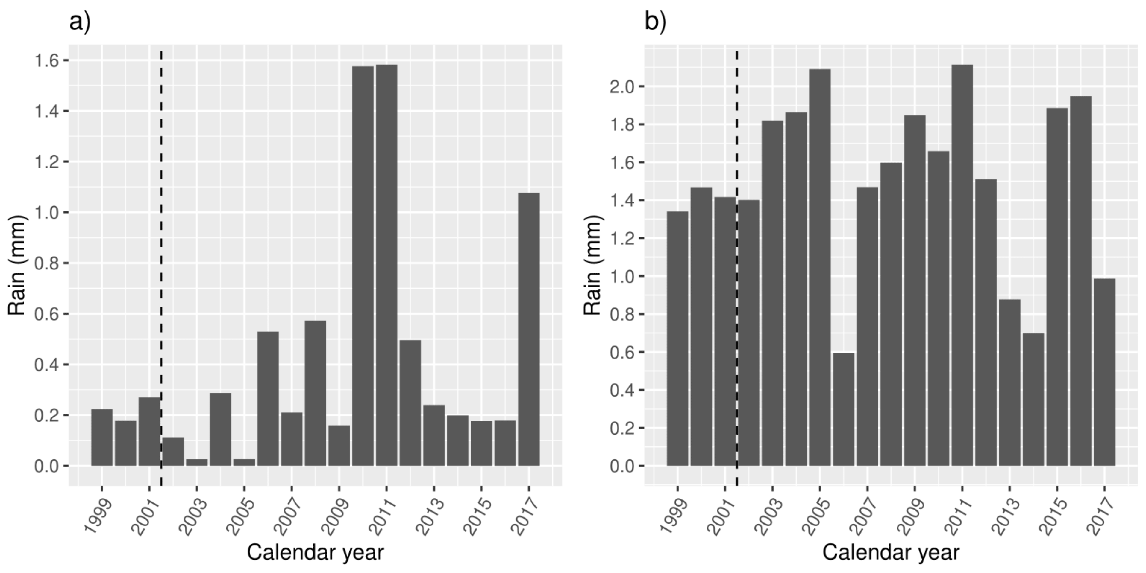
2.4. Rainfall Data
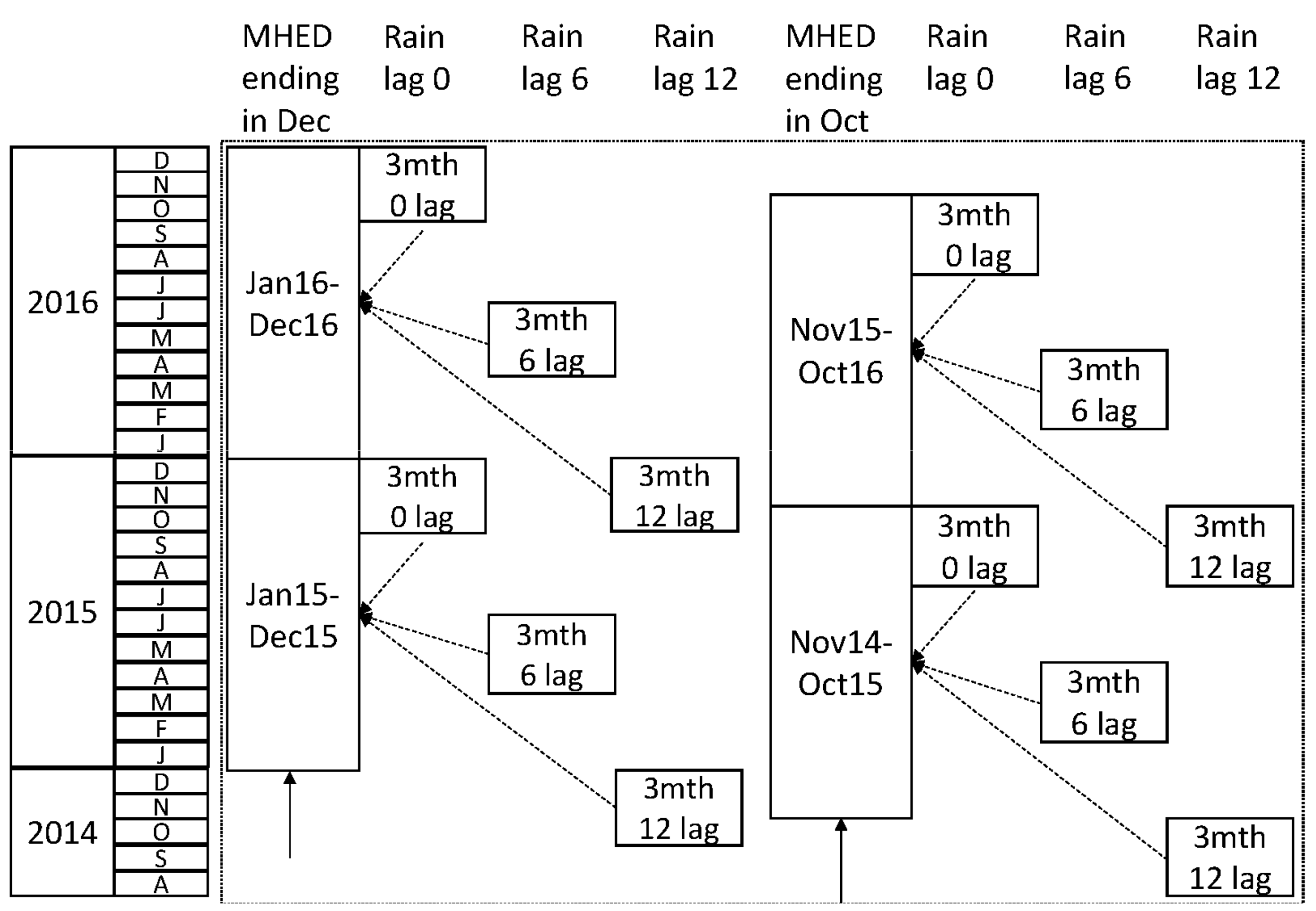
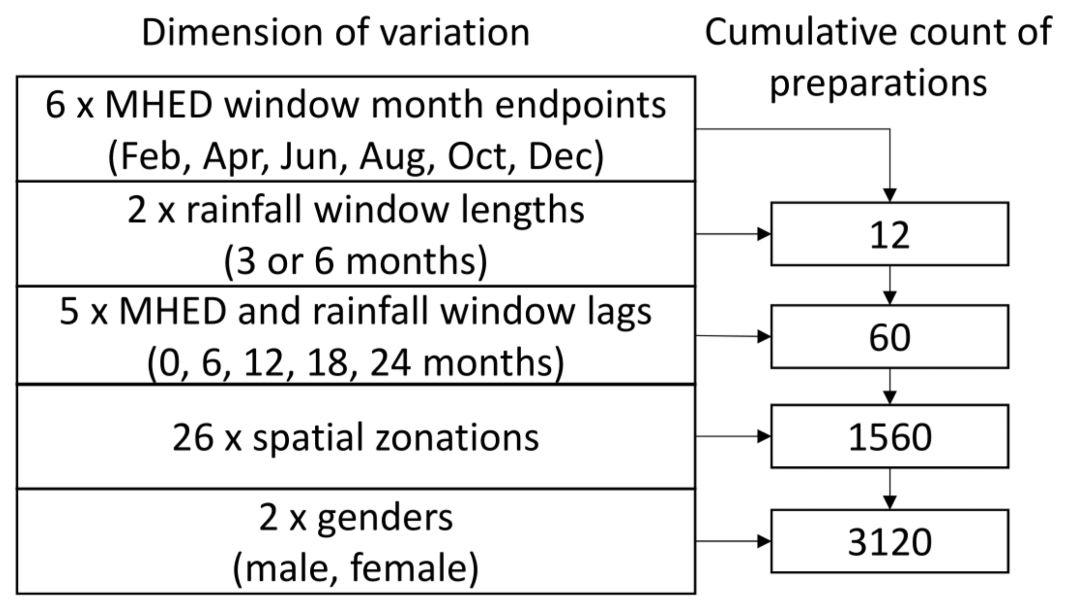
2.5. Data Preparation
2.6. Statistical Models
2.7. Ethical Approval
3. Results
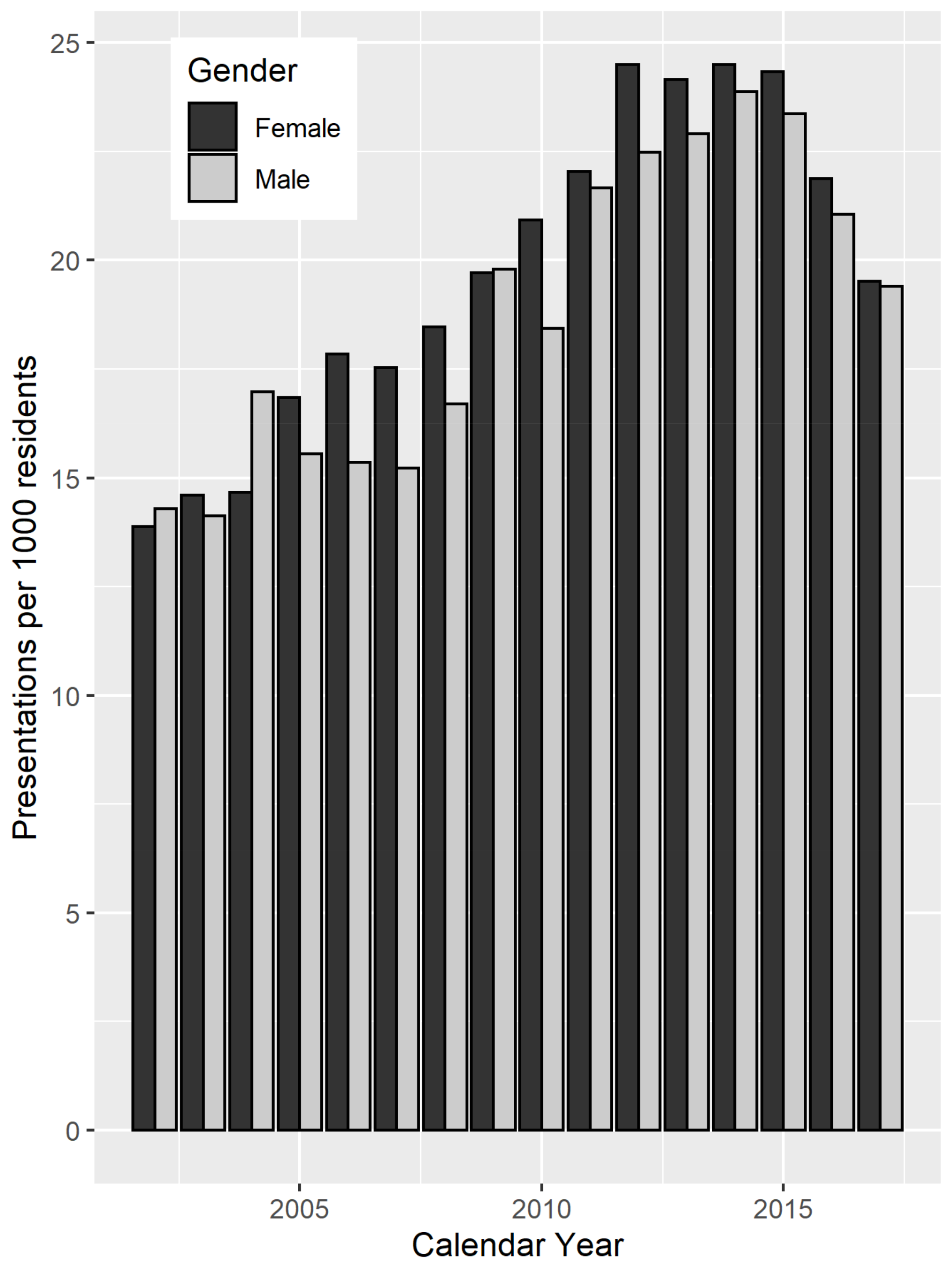
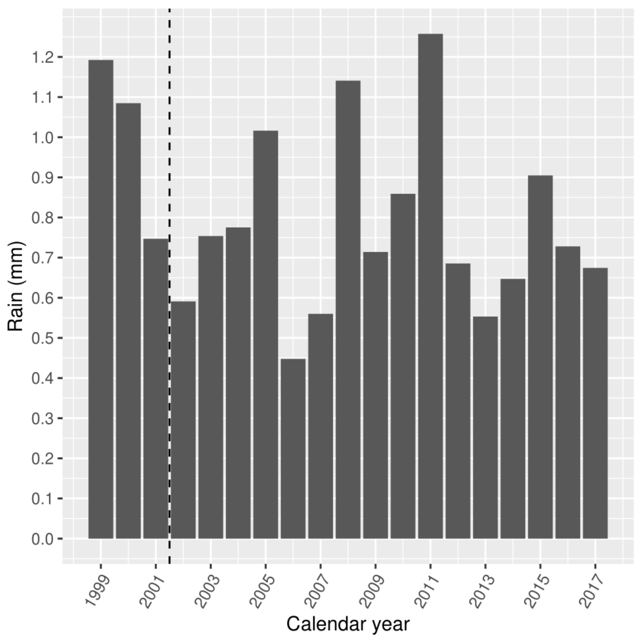
3.1. Summary Characteristics
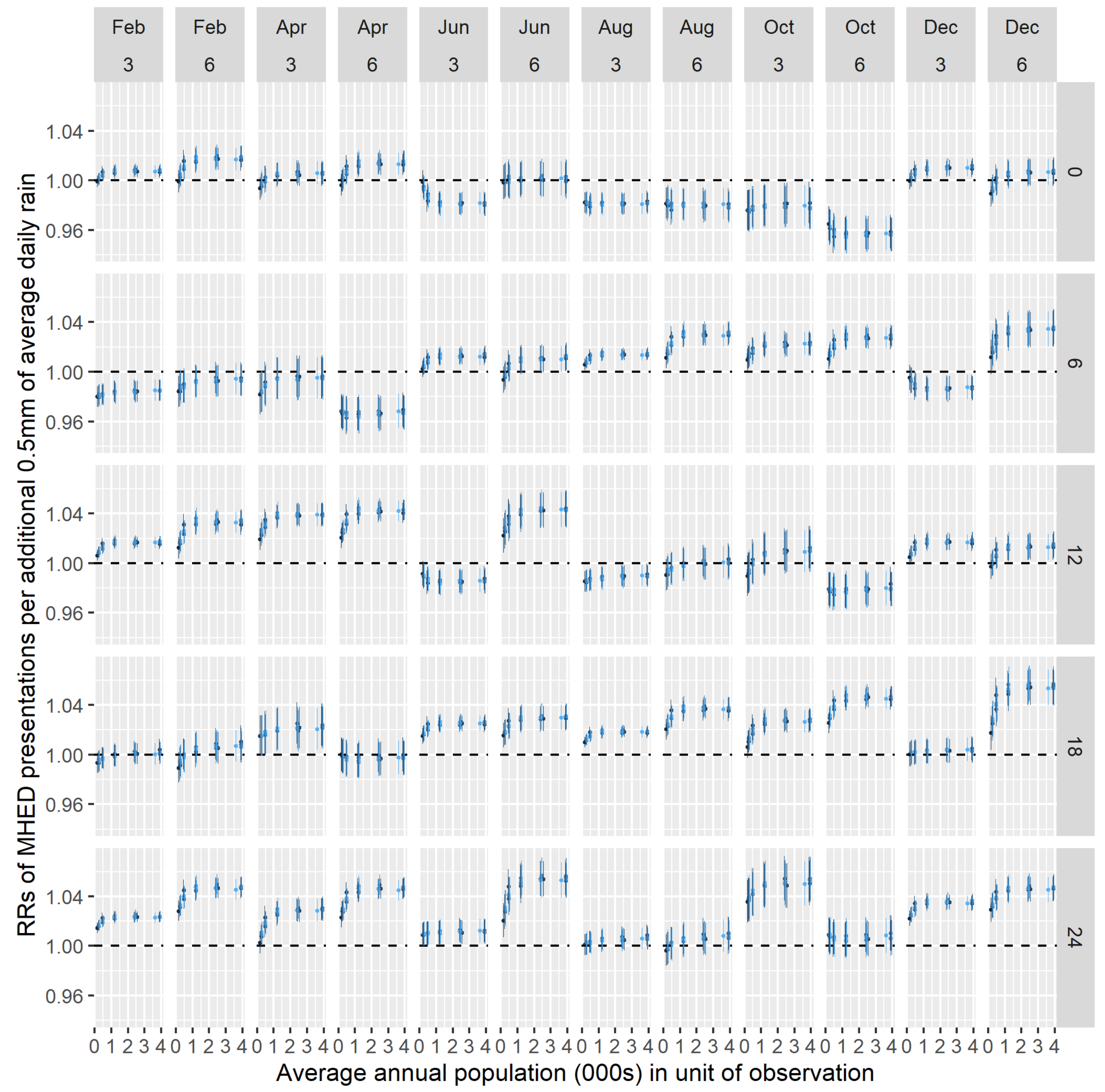
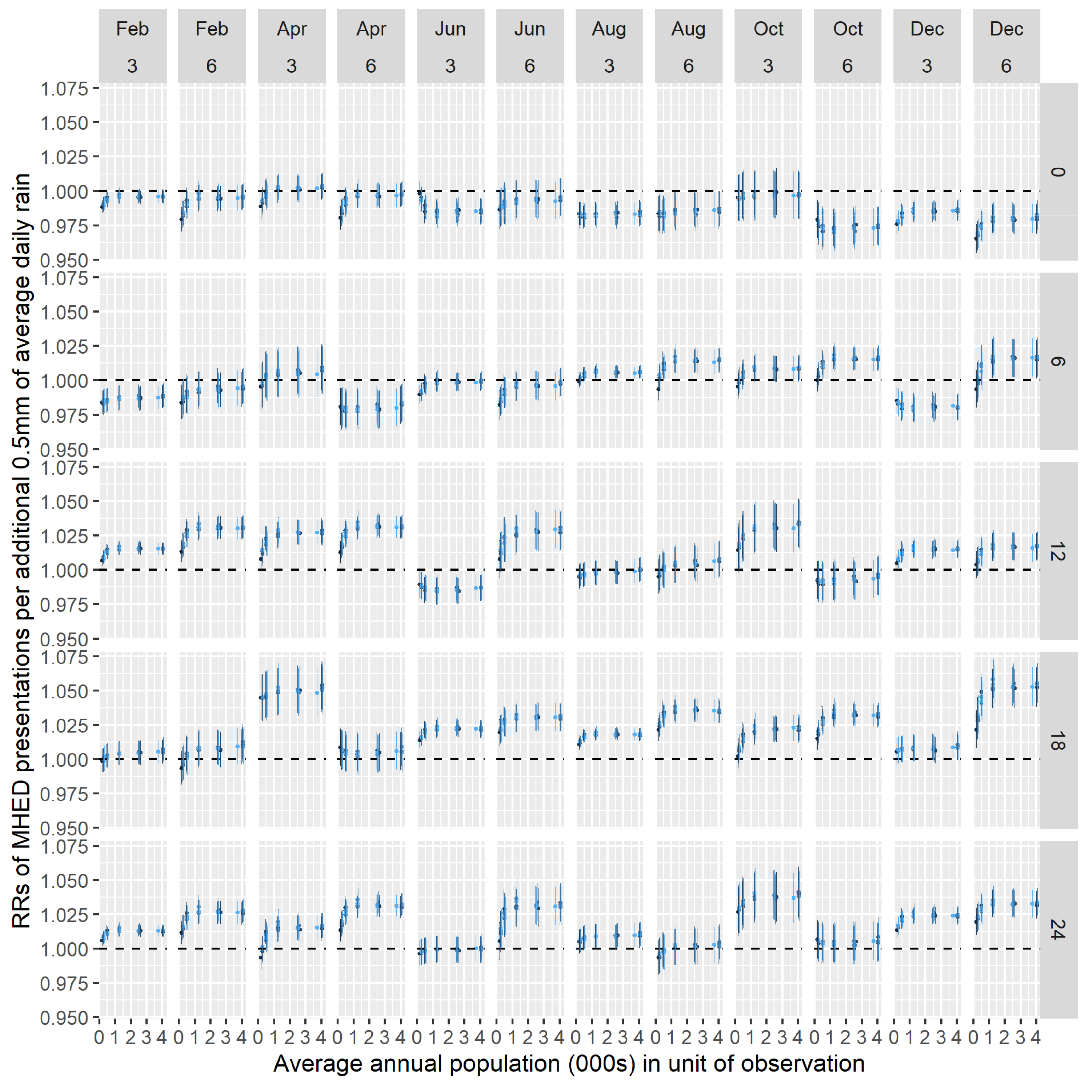
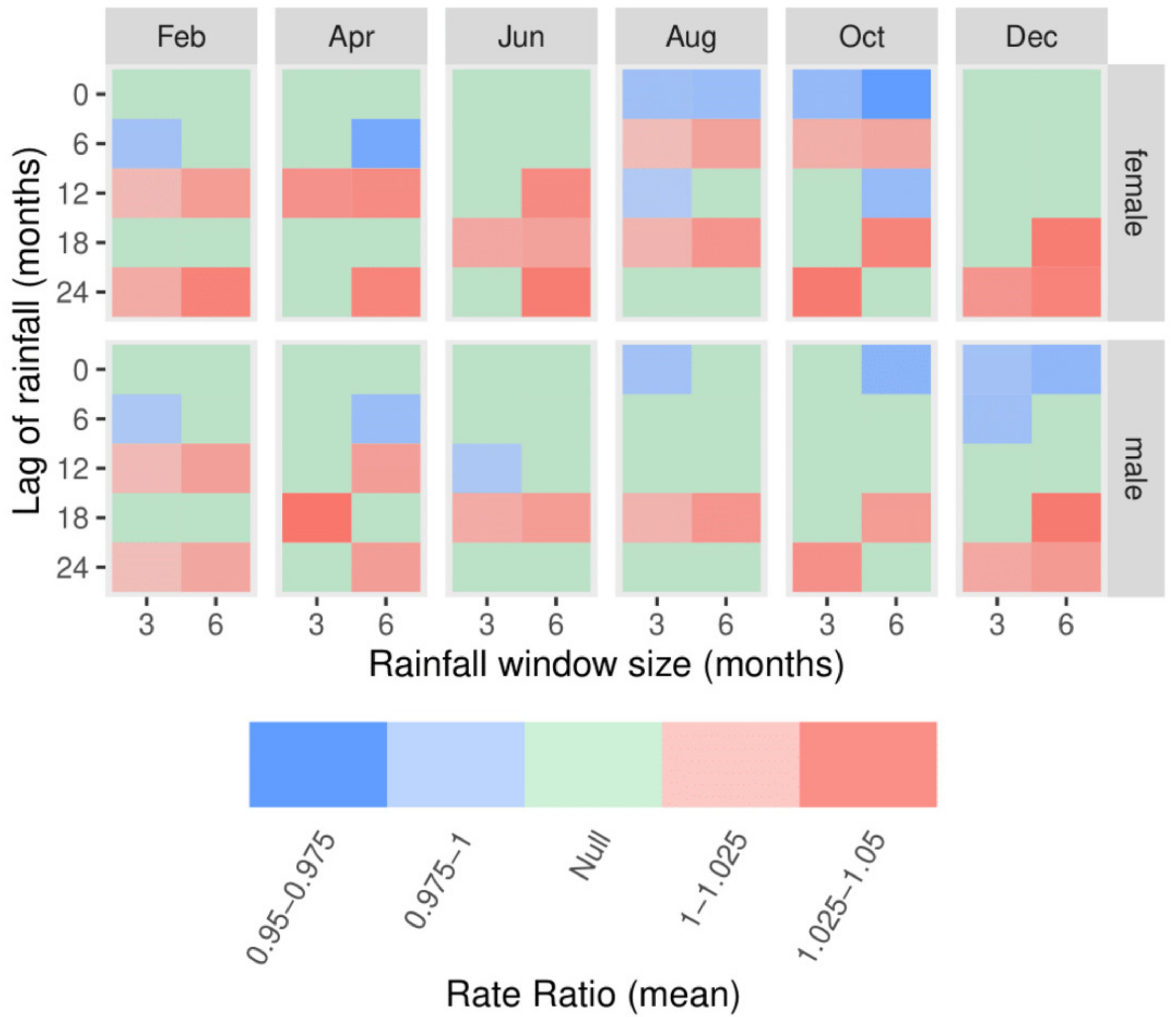
3.2. Model Results
4. Discussion
5. Conclusions
Author Contributions
Funding
Institutional Review Board Statement
Informed Consent Statement
Data Availability Statement
Acknowledgments
Conflicts of Interest
References
- Ritchie, H.; Roser, M. Mental Health. Available online: https://ourworldindata.org/mental-health (accessed on 3 July 2020).
- Australian Institute of Health and Welfare. Australian Burden of Disease Study: Impact and Causes of Illness and Death in Australia 2015; AIHW: Canberra, ACT, Australia, 2019. [Google Scholar]
- Yap, M.; Tuson, M.; Whyatt, D.; Vickery, A. Anxiety and alcohol in the working-age population are driving a rise in mental health-related emergency department presentations: 15 year trends in emergency department presentations in Western Australia. Emerg. Med. Australas. 2020, 32, 80–87. [Google Scholar] [CrossRef] [PubMed]
- Tran, Q.N.; Lambeth, L.G.; Sanderson, K.; de Graaff, B.; Breslin, M.; Huckerby, E.J.; Tran, V.; Neil, A.L. Trend of emergency department presentations with a mental health diagnosis in Australia by diagnostic group, 2004–2005 to 2016–17. Emerg. Med. Australas. 2020, 32, 190–201. [Google Scholar] [CrossRef] [PubMed]
- Stanke, C.; Kerac, M.; Prudhomme, C.; Medlock, J.; Murray, V. Health effects of drought: A systematic review of the evidence. PLoS Curr. 2013, 5. [Google Scholar] [CrossRef] [PubMed] [Green Version]
- Vins, H.; Bell, J.; Saha, S.; Hess, J.J. The mental health outcomes of drought: A systematic review and causal process diagram. Int. J. Eviron. Res. Public Health 2015, 12, 13251–13275. [Google Scholar] [CrossRef] [Green Version]
- Edwards, B.; Gray, M.; Hunter, B. The impact of drought on mental health in rural and regional Australia. Soc. Indic. Res. 2015, 121, 177–194. [Google Scholar] [CrossRef]
- O’Brien, L.V.; Berry, H.L.; Coleman, C.; Hanigan, I.C. Drought as a mental health exposure. Environ. Res. 2015, 131, 180–187. [Google Scholar] [CrossRef] [Green Version]
- Dean, G.D.; Stain, H.J. Mental health impact for adolescents living with prolonged drought. Aust. J. Rural Health 2010, 18, 32–37. [Google Scholar] [CrossRef]
- Powers, J.R.; Loxton, D.; Baker, J.; Rich, J.L.; Dobson, A.J. Empirical evidence suggests adverse climate events have not affected Australian women’s health and well-being. Aust. N.Z. J. Public Health 2012, 36, 452–457. [Google Scholar] [CrossRef] [Green Version]
- Austin, E.K.; Handley, T.; Kiem, A.S.; Rich, J.L.; Lewin, T.J.; Askland, H.H.; Askarimarnani, S.S.; Perkins, D.A.; Kelly, B.J. Drought-related stress among farmers: Findings from the Australian Rural Mental Health Study. MJA 2018, 209, 159–165. [Google Scholar] [CrossRef]
- Althubaiti, A. Information bias in health research: Definition, pitfalls, and adjustment methods. J. Multidiscip. Healthc. 2016, 9, 211–217. [Google Scholar] [CrossRef] [Green Version]
- Hanigan, I.C.; Butler, C.D.; Kokic, P.N.; Hutchinson, M.F. Suicide and drought in New South Wales, Australia, 1970–2007. Proc. Natl. Acad. Sci. USA 2012, 109, 13950–13955. [Google Scholar] [CrossRef] [PubMed] [Green Version]
- Cheng, T.; Adepeju, M. Modifiable Temporal Unit Problem (MTUP) and Its Effect on Space-Time Cluster Detection. PLoS ONE 2014, 9. [Google Scholar] [CrossRef] [PubMed] [Green Version]
- Tuson, M.; Yap, M.; Kok, M.R.; Murray, K.; Turlach, B.A.; Whyatt, D. Incorporating geography into a new generalized theoretical and statistical framework addressing the modifiable areal unit problem. Int. J. Health Geogr. 2019, 18, 6. [Google Scholar] [CrossRef] [PubMed] [Green Version]
- Openshaw, S.; Taylor, P.J. A million or so correlation coefficients: Three experiments on the modifiable areal unit problem. In Statistical Applications in the Spatial Sciences; Wrigley, N., Ed.; Pion: London, UK, 1979; Volume 127, Chapter 5; pp. 127–144. [Google Scholar]
- Gehlke, C.E.; Biehl, K. Certain effects of grouping upon the size of the correlation coefficient in census tract material. J. Am. Stat. Assoc. 1934, 29, 169–170. [Google Scholar]
- Manley, D. Scale, aggregation, and the modifiable areal unit problem. In The Handbook of Regional Science; Fischer, M.M., Nijkamp, P., Eds.; Springer: Berlin, Germany, 2014; Chapter 59; pp. 1157–1171. [Google Scholar]
- Department of Agriculture, Water and the Environment. Catchment Scale Land Use of Australia. Available online: https://www.agriculture.gov.au/abares/aclump/land-use/land-use-mapping (accessed on 9 July 2020).
- Wilkinson, I. Western Australian Wheat Industry. Available online: https://www.agric.wa.gov.au/grains-research-development/western-australian-wheat-industry (accessed on 9 July 2020).
- Australian Bureau of Statistics. Australian Statistical Geography Standard (ASGS) Volume 1—Main Structure and Greater Capital City Statistical Area; Catalogue number 1270.0.55.001; ABS: Canberra, ACT, Australia, 2016.
- Australian Bureau of Statistics. Census of Population and Housing—Counting Persons, Place of Usual Residence (SA1), TableBuilder; Findings based on use of ABS TableBuilder Data; ABS: Canberra, ACT, Australia, 2016.
- Holman, C.A.J.; Bass, A.J.; Rouse, I.L.; Hobbs, M.S.T. Population-based linkage of health records in Western Australia: Development of a health services research linked database. Aust. N.Z. J. Public Health 1999, 23, 453–459. [Google Scholar] [CrossRef] [PubMed]
- National Centre for Classification in Health. The International Statistical Classification of Diseases and Related Health Problems, Tenth Revision, Australian Modification (ICD-10-AM), 7th ed.; National Centre for Classification in Health: Lidcombe, NSW, Australia, 2010. [Google Scholar]
- Bureau of Meteorology. Gridded Daily Global Precipitation; Bureau of Meteorology: Melbourne, VIC, Australia, 2019.
- Martin, D. Extending the automated zoning procedure to reconcile incompatible zoning systems. Int. J. Geogr. Inf. Sci. 2003, 17, 181–196. [Google Scholar] [CrossRef] [Green Version]
- Cockings, S.; Harfoot, A.; Martin, D.; Hornby, D. Maintaining Existing Zoning Systems Using Automated Zone-Design Techniques: Methods for Creating the 2011 Census Output Geographies for England and Wales. Environ. Plan A Econ. Space 2011, 43, 2399–2418. [Google Scholar] [CrossRef]
- Besag, J.; York, J.; Mollié, A. Bayesian image restoration, with two applications in spatial statistics. Ann. Inst. Stat. Math. 1991, 43, 1–20. [Google Scholar] [CrossRef]
- Rue, H.; Martino, S.; Chopin, N. Approximate Bayesian inference for latent Gaussian models using integrated nested Laplace approximations (with discussion). J. R. Stat. Soc. Ser. B 2009, 71, 319–392. Available online: https://r-inla.org/ (accessed on 10 September 2019). [CrossRef]
- Martin, T.; Simpson, D.; Lindgren, F.; Rue, H. Bayesian computing with INLA: New features. Comp. Stat. Data Anal. 2013, 67, 68–83. [Google Scholar] [CrossRef] [Green Version]
- R Core Team. R: A Language and Environment for Statistical Computing; R Foundation for Statistical Computing: Vienna, Austria, 2019; Available online: https://www.R-project.org/ (accessed on 22 June 2019).
- Cramb, S.; Mengersen, K.; Baade, P.D. Developing the atlas of cancer in Queensland: Methodological issues. Int. J. Health Geogr. 2011, 10, 9. [Google Scholar] [CrossRef] [PubMed] [Green Version]
- Blangiardo, M.; Cameletti, M.; Baio, G.; Rue, H. Spatial and spatio-temporal models with r-INLA. Spat. Spatio-Temporal Epidemiol. 2013, 7, 39–55. [Google Scholar] [CrossRef] [PubMed] [Green Version]
- CSIRO. State of the Climate 2018. Bureau of Meteorology, Australian Government 2018. Available online: www.csiro.au/state-of-the-climate (accessed on 2 December 2020).
- Sarto, M.V.; Sarto, J.R.; Rampim, L.; Rosset, J.S.; Bassegio, D.; Costa, P.F.; Inagaki, A.M. Wheat phenology and yield under drought: A review. Aust. J. Crop Sci. 2017, 11, 941–946. [Google Scholar] [CrossRef]
- Albrecht, G.; Sartore, G.M.; Connor, L.; Higginbotham, N.; Freeman, S.; Kelly, B.; Stain, H.; Tonna, A.; Pollard, G. Solastalgia: The distress caused by environmental change. Australas. Psychiatry 2007, 15 (Suppl. 1), S95–S98. [Google Scholar] [CrossRef]
- CBH Group 2016. Department of Agriculture, Water and the Environment. CBH Submission: Working Holiday Maker Visa Review. Available online: https://www.agriculture.gov.au/sites/default/files/sitecollectiondocuments/ag-food/working-holiday/submissions/cbh-group.pdf (accessed on 5 May 2020).
- Bhaskaran, K.; Gasparrini, A.; Hajat, S.; Smeeth, L.; Armstrong, B. Time series regression studies in environmental epidemiology. Int. J. Epidemiol. 2013, 42, 1187–1195. [Google Scholar] [CrossRef]
- Ahsan, F.; Chandio, A.A.; Fang, W. Climate change impacts on cereal crops production in Pakistan: Evidence from cointegration analysis. Int. J. Clim. Change Strateg. Manag. 2020, 12, 257–269. [Google Scholar] [CrossRef]
- Asseng, S.; Foster, I.; Turner, N.C. The impact of temperature variability on wheat yields. Glob. Change Biol. 2011, 17, 997–1012. [Google Scholar] [CrossRef]
- Grains Industry Association of Western Australia. 2019 Season Crop Report. February 2020. Available online: http://www.giwa.org.au/2019 (accessed on 26 June 2020).
- Wilhite, D.A.; Glantz, M.H. Understanding the Drought Phenomenon: The Role of Definitions; Drought Mitigation Center Faculty Publications: Lincoln, NE, USA, 1985. [Google Scholar]
- Grant, W.B. The role of geographical ecological studies in identifying diseases linked to UVB exposure and/or vitamin D. Dermatoendocrinology 2016, 8. [Google Scholar] [CrossRef] [Green Version]
- Lobonţ, O.R.; Nicolescu, A.C.; Moldovan, N.C.; Kuloğlu, A. The effect of socioeconomic factors on crime rates in Romania: A macro-level analysis. Econ. Res. 2017, 30, 91–111. [Google Scholar] [CrossRef]
- Rural Business Development Unit, Department of Agriculture and Food, Western Australia. The Evolution of Drought Policy in Western Australia; Western Australian Agriculture Authority: South Perth, WA, Australia, 2014.


| Resident Characteristics | |
|---|---|
| Mean age (SD) | 38.5 (1.4) |
| Mean percentile SES (SD) | 33.3 (4.6) |
| Mean population per square km (SD) | 0.6 (0.02) |
| Percent male | 50.8 |
| Mean annual resident population (SD) | 188,001 (5040) |
| MHED Characteristics | |
| Mean age of patients (SD) | 36.9 (16.6) |
| Percent male | 49.6 |
| Mean annual MHED presentations (SD) | 3682 (822) |
Publisher’s Note: MDPI stays neutral with regard to jurisdictional claims in published maps and institutional affiliations. |
© 2021 by the authors. Licensee MDPI, Basel, Switzerland. This article is an open access article distributed under the terms and conditions of the Creative Commons Attribution (CC BY) license (http://creativecommons.org/licenses/by/4.0/).
Share and Cite
Yap, M.; Tuson, M.; Turlach, B.; Boruff, B.; Whyatt, D. Modelling the Relationship between Rainfall and Mental Health Using Different Spatial and Temporal Units. Int. J. Environ. Res. Public Health 2021, 18, 1312. https://0-doi-org.brum.beds.ac.uk/10.3390/ijerph18031312
Yap M, Tuson M, Turlach B, Boruff B, Whyatt D. Modelling the Relationship between Rainfall and Mental Health Using Different Spatial and Temporal Units. International Journal of Environmental Research and Public Health. 2021; 18(3):1312. https://0-doi-org.brum.beds.ac.uk/10.3390/ijerph18031312
Chicago/Turabian StyleYap, Matthew, Matthew Tuson, Berwin Turlach, Bryan Boruff, and David Whyatt. 2021. "Modelling the Relationship between Rainfall and Mental Health Using Different Spatial and Temporal Units" International Journal of Environmental Research and Public Health 18, no. 3: 1312. https://0-doi-org.brum.beds.ac.uk/10.3390/ijerph18031312