
A Bi-Objective Home Health Care Routing and Scheduling Model with Considering Nurse Downgrading Costs


Abstract
:1. Introduction
2. Problem Description
2.1. Assumptions
- Several different service needs and qualifications are included in the problem.
- All service needs of patients should be provided by qualified nurses.
- Each route of a nurse is started from the depot.
- Each nurse should end its path at the depot after visiting all planned patients.
- Each patient’s acceptable time window should be respected.
- The parameters of the patient demand, traveling time, and service time are known before the planning and considered to be deterministic.
- The correct servicing sequence of each nurse should be respected by considering the service time of the previous patient in addition to the time needed for traveling between the patients’ places.
- A single period planning strategy is considered in the problem.
- Travel sharing and multi-mode traveling concepts are not considered.
- Emergent situations and urgent service needs are not included in the problem.
2.2. Notations
2.2.1. Subscripts
| i | Starting node index of each travel (i = 1, 2, ..., n + 1), where n denotes the number of patients in the planning. |
| j | Ending node index of each travel (j = 2, 3, ..., n + 2), where n denotes the number of patients in the planning. |
| k | Index for the nurses (k = 1, 2, …, V), where V denotes the number of nurses in the planning. |
| s | Index for the services (s = 1, 2, …, S), where S denotes the number of different services in the planning. |
2.2.2. Sets
| C | Set of patients. |
| N | Set of all nodes that includes patients and the depot. |
| V | Set of nurses. |
| S | Set of services. |
2.2.3. Input Parameters
| tij | Travel time between node i and node j. |
| tis | Required time for offering service s to patient i. |
| li | Lower bound on the patient time window. |
| ui | Upper bound on the patient time window. |
| Input matrix of nurse qualifications, where 1 means that nurse k has the qualification of doing service s. | |
| Input matrix of patient’s service needs, where 1 means that patient j needs service s. | |
| Weighted value of service s for the decision-maker. | |
| A small positive number, e.g., 0.1. |
2.3. Decision Variables
| 1 if nurse k transfers from node i to j for offering service s; 0 otherwise. | |
| Starting time of offering service s to patient i by nurse k. | |
| 1 if service s of nurse k is used in the optimal planning; 0 otherwise. |
2.4. The Mathematical Model
2.4.1. Objective Function
2.4.2. Constraints
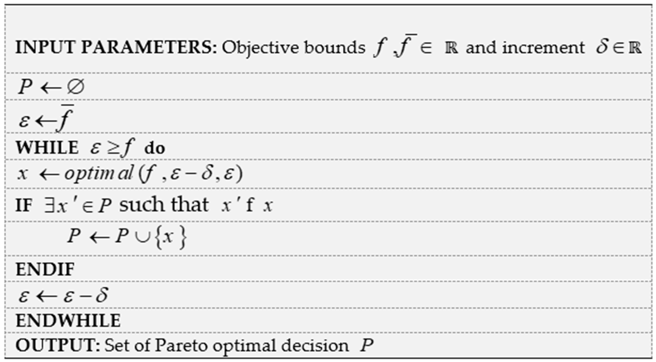
3. Solution Approach
3.1. Background
3.2. Proposed Solution Approach
4. Computational Experiments
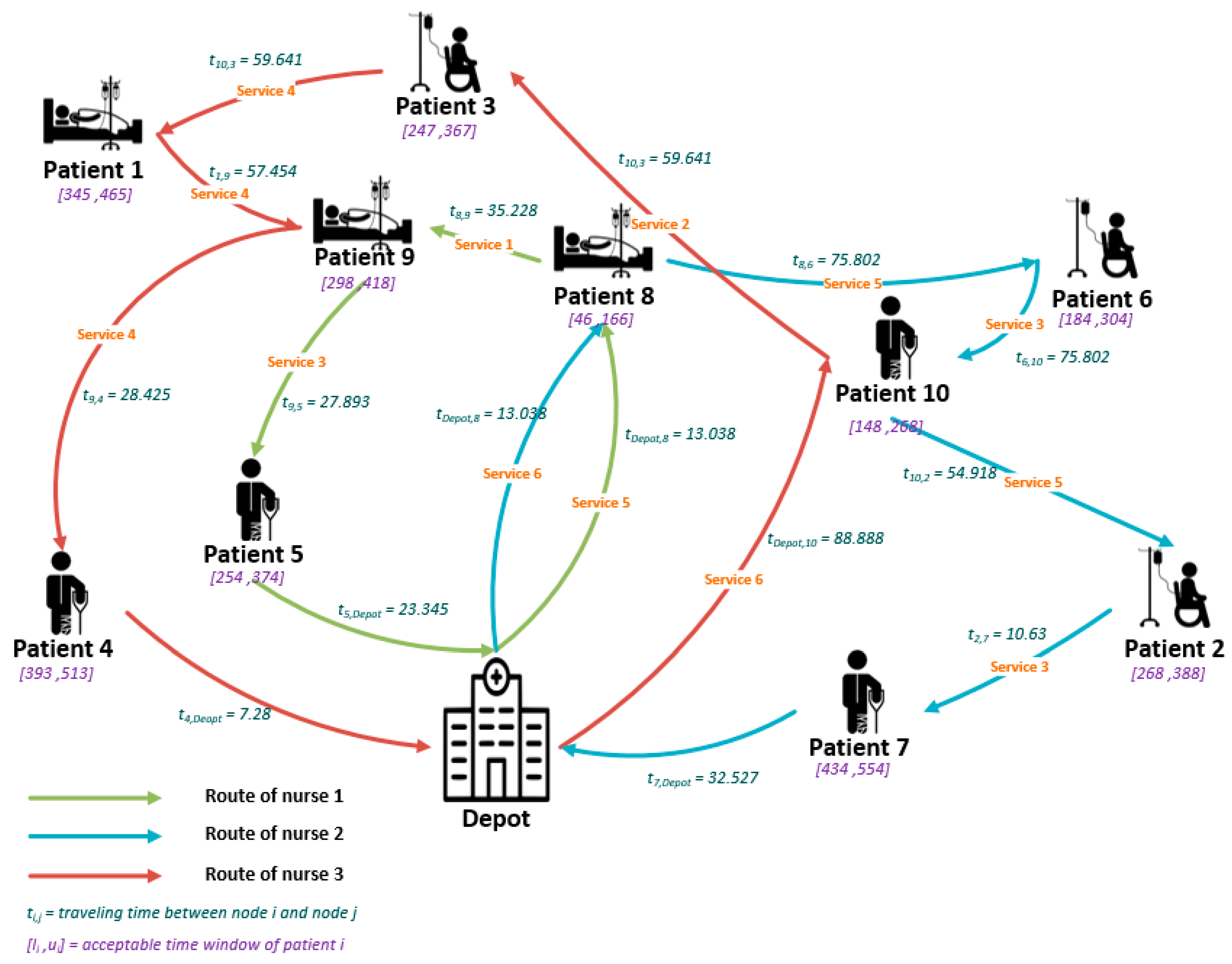
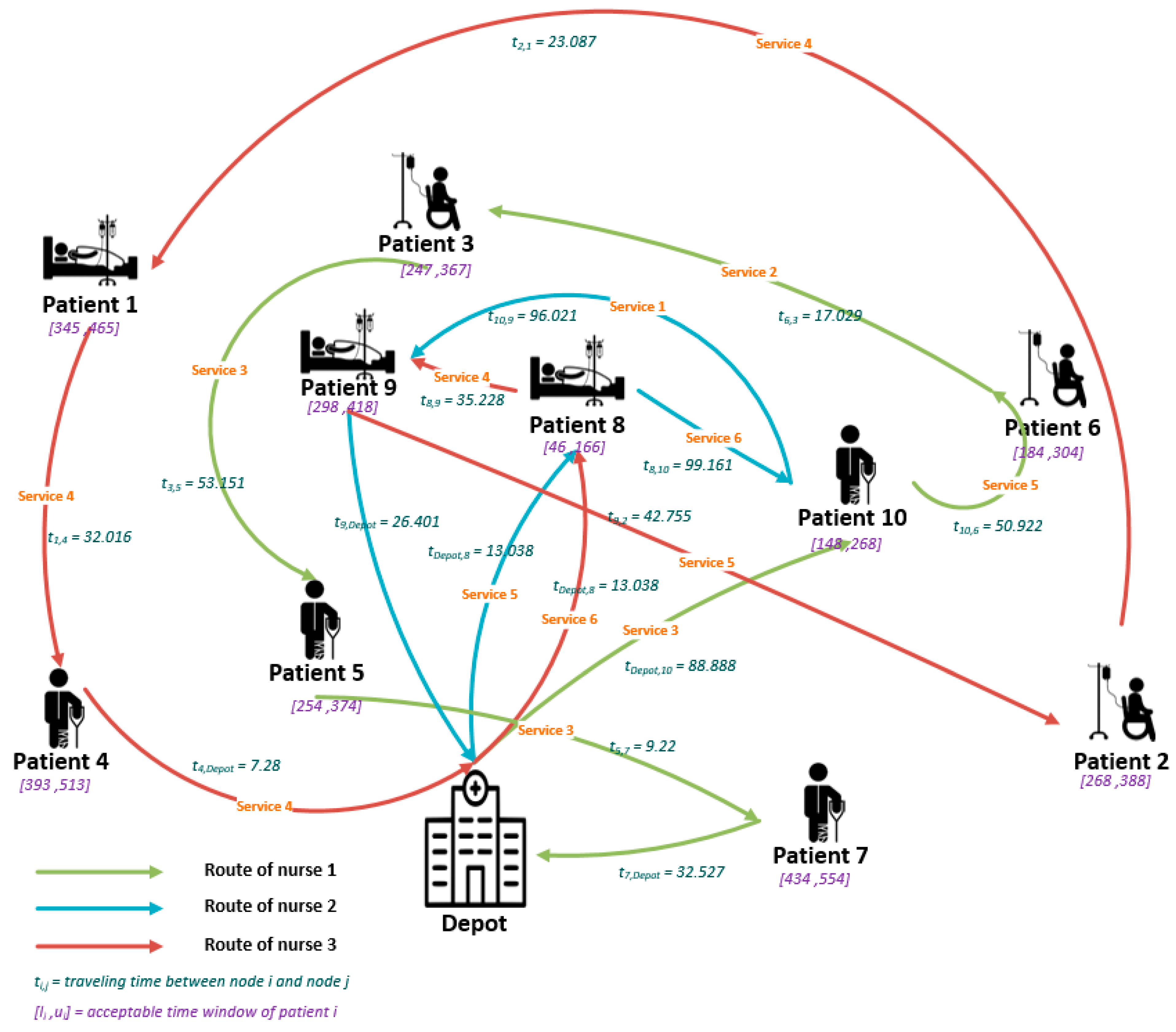
4.1. Planning Process
4.2. Results
4.3. Sensitivity Analysis
4.3.1. Effect of the Epsilon Parameter on the Optimal Solution Value
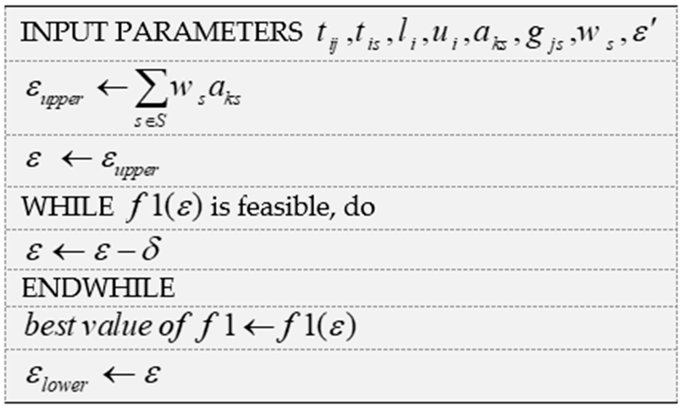
4.3.2. Upper Limit for the Meaningful Epsilon Parameter
5. Managerial Insights
- This novel mathematical model could be used by managers for better planning of the company’s nurses considering downgrading aspects. The managers could make an appropriate trade-off between downgrading and total traveling times of the nurses. The downgrading level could be adjusted by changing the Epsilon parameter of the model.
- In most traditional home health care routing and scheduling models, the home health care decision-maker assumes that each patient requires only one type of service. In fact, if a patient needs three services simultaneously, the plan considers it as three different patients who have the same place and health profile. The managers of the health care industry can decrease the volume of data in their companies by using this new method as well. Actually, in this plan, each patient has a unique physical and health profile, where besides removing multiple same profiles for each patient, the home health care company can have a clean and rich database from their customers. In addition, top-level managers can use this valuable resource to establish marketing strategies or manage their employees and service capacities.
- Downgrading concepts could help the managers for making better nurse capability decisions. The managers could understand that there are some unrequired nurse qualifications in their company or there are extra needs for new skills, and he/she should hire additional skillful nurses for getting a better service level to the patients.
6. Conclusions and Future Studies
Author Contributions
Funding
Institutional Review Board Statement
Informed Consent Statement
Data Availability Statement
Conflicts of Interest
Appendix A

| Patient Number | Service Needs | Acceptable Time Windows |
|---|---|---|
| 1 | S4 | (345,465) |
| 2 | S5 | (268,388) |
| 3 | S2 | (247,367) |
| 4 | S4 | (393,513) |
| 5 | S3 | (254,374) |
| 6 | S5 | (184,304) |
| 7 | S3 | (434,554) |
| 8 | S5, S6 | (46,166) |
| 9 | S1, S4 | (298,418) |
| 10 | S3, S6 | (148,268) |
| Depot | 1 | 2 | 3 | 4 | 5 | 6 | 7 | 8 | 9 | 10 | |
|---|---|---|---|---|---|---|---|---|---|---|---|
| Depot | 0 | 38.471 | 34.886 | 55.946 | 7.28 | 23.345 | 71.47 | 32.527 | 13.038 | 26.401 | 88.888 |
| 1 | 38.471 | 0 | 23.087 | 21.401 | 32.016 | 31.828 | 34 | 32.65 | 45.277 | 57.454 | 56.859 |
| 2 | 34.886 | 23.087 | 0 | 43.829 | 27.785 | 15.033 | 53.038 | 10.63 | 46.615 | 42.755 | 54.918 |
| 3 | 55.946 | 21.401 | 43.829 | 0 | 50.606 | 53.151 | 17.029 | 53.852 | 59.228 | 77.801 | 59.641 |
| 4 | 7.28 | 32.016 | 27.785 | 50.606 | 0 | 17.493 | 65.552 | 26.401 | 19.105 | 28.425 | 81.609 |
| 5 | 23.345 | 31.828 | 15.033 | 53.151 | 17.493 | 0 | 65 | 9.22 | 36.235 | 27.893 | 69.584 |
| 6 | 71.47 | 34 | 53.038 | 17.029 | 65.552 | 65 | 0 | 63.64 | 75.802 | 91.417 | 50.922 |
| 7 | 32.527 | 32.65 | 10.63 | 53.852 | 26.401 | 9.22 | 63.64 | 0 | 45.343 | 34.015 | 62.073 |
| 8 | 13.038 | 45.277 | 46.615 | 59.228 | 19.105 | 36.235 | 75.802 | 45.343 | 0 | 35.228 | 99.161 |
| 9 | 26.401 | 57.454 | 42.755 | 77.801 | 28.425 | 27.893 | 91.417 | 34.015 | 35.228 | 0 | 96.021 |
| 10 | 88.888 | 56.859 | 54.918 | 59.641 | 81.609 | 69.584 | 50.922 | 62.073 | 99.161 | 96.021 | 0 |
| Service ID | Service Type | Supposed Weighted Value |
|---|---|---|
| S1 | Speech therapy | 1 |
| S2 | Wound dressing | 2 |
| S3 | Insulin injection | 3 |
| S4 | Blood sampling | 4 |
| S5 | Physiotherapy | 5 |
| S6 | X-ray imaging | 6 |
| Nurse Number | Service Qualifications |
|---|---|
| 1 | S1, S2, S3, S5 |
| 2 | S1, S3, S5, S6 |
| 3 | S2, S4, S5, S6 |
Appendix B
| Patient Number | Service Needs | Acceptable Time Windows |
|---|---|---|
| 1 | S4 | (345,465) |
| 2 | S5 | (268,388) |
| 3 | S2 | (247,367) |
| 4 | S4 | (393,513) |
| 5 | S3 | (254,374) |
| 6 | S5 | (184,304) |
| 7 | S3 | (434,554) |
| 8 | S5 | (46,166) |
| 9 | S5 | (298,418) |
| 10 | S5 | (148,268) |
| 11 | S2 | (409,529) |
| 12 | S2 | (73,193) |
| 13 | S2 | (157,277) |
| 14 | S4 | (63,183) |
| 15 | S1 | (282,403) |
| 16 | S5 | (274,394) |
| 17 | S3 | (152,272) |
| 18 | S5, S6 | (222,342) |
| 19 | S5, S6 | (276,396) |
| 20 | S4, S6 | (29,149) |
| 21 | S5, S6 | (416,536) |
| 22 | S2, S4 | (332,452) |
| 23 | S2, S6 | (190,310) |
| 24 | S1, S4 | (59,179) |
| 25 | S1, S4 | (434,554) |
| Depot | 1 | 2 | 3 | 4 | 5 | 6 | 7 | 8 | 9 | 10 | 11 | 12 | 13 | 14 | 15 | 16 | 17 | 18 | 19 | 20 | 21 | 22 | 23 | 24 | 25 | |
|---|---|---|---|---|---|---|---|---|---|---|---|---|---|---|---|---|---|---|---|---|---|---|---|---|---|---|
| Depot | 0 | 49.041 | 39.205 | 51.088 | 34.713 | 45.88 | 68.264 | 35.468 | 7.28 | 33.838 | 9.22 | 75.007 | 35.735 | 33.615 | 66.483 | 91.302 | 85.212 | 25.06 | 13.601 | 27.857 | 70.349 | 16.125 | 15.264 | 65.276 | 87.321 | 85.024 |
| 1 | 49.041 | 0 | 9.899 | 30.871 | 31.145 | 25.06 | 39.051 | 15.524 | 53.535 | 49.01 | 43.932 | 48.918 | 27.166 | 51 | 18.028 | 43.966 | 53.235 | 24.839 | 45.695 | 28.443 | 40 | 34.482 | 34.986 | 36.797 | 48.27 | 57.428 |
| 2 | 39.205 | 9.899 | 0 | 29 | 26 | 24.207 | 41.146 | 8.544 | 43.909 | 42.755 | 34.059 | 50.606 | 22.361 | 44.553 | 27.803 | 52.924 | 56.921 | 15 | 36.688 | 21.095 | 42.544 | 25.08 | 25.495 | 38.471 | 54.148 | 59.933 |
| 3 | 51.088 | 30.871 | 29 | 0 | 53.824 | 53.151 | 17.263 | 36.878 | 58.009 | 68.447 | 42.297 | 24.331 | 50.606 | 69.857 | 43.105 | 50.22 | 34.132 | 30.364 | 55.902 | 47.011 | 19.416 | 44.385 | 44.147 | 14.318 | 38.013 | 34.366 |
| 4 | 34.713 | 31.145 | 26 | 53.824 | 0 | 12.728 | 67.119 | 17.464 | 34.928 | 18.111 | 36.056 | 76.479 | 4 | 20.224 | 42.72 | 73.682 | 82.873 | 26.627 | 23.707 | 8.544 | 68.542 | 20.025 | 21.024 | 64.405 | 79.246 | 85.907 |
| 5 | 45.88 | 25.06 | 24.207 | 53.151 | 12.728 | 0 | 63.82 | 17.464 | 47.011 | 29.155 | 45.541 | 73.6 | 10.296 | 31.385 | 32.14 | 64.008 | 78.294 | 31.575 | 36.056 | 18.028 | 64.9 | 30.083 | 31.048 | 61.4 | 72.732 | 82.377 |
| 6 | 68.264 | 39.051 | 41.146 | 17.263 | 67.119 | 63.82 | 0 | 49.659 | 75.107 | 83.169 | 59.54 | 9.899 | 63.506 | 84.77 | 44.721 | 39.85 | 17 | 46.39 | 72.339 | 61.351 | 2.236 | 60.531 | 60.407 | 3 | 22.023 | 18.788 |
| 7 | 35.468 | 15.524 | 8.544 | 36.878 | 17.464 | 17.464 | 49.659 | 0 | 39.051 | 34.366 | 32.202 | 59.059 | 13.892 | 36.222 | 31.401 | 59.481 | 65.46 | 15.033 | 30.414 | 13.038 | 51.078 | 19.849 | 20.518 | 46.957 | 62.394 | 68.447 |
| 8 | 7.28 | 53.535 | 43.909 | 58.009 | 34.928 | 47.011 | 75.107 | 39.051 | 0 | 30.265 | 16.492 | 82.055 | 36.715 | 29.614 | 70.434 | 96.607 | 92.087 | 30.676 | 11.402 | 29.411 | 77.162 | 19.209 | 18.601 | 72.111 | 93.744 | 92.087 |
| 9 | 33.838 | 49.01 | 42.755 | 68.447 | 18.111 | 29.155 | 83.169 | 34.366 | 30.265 | 0 | 39.446 | 92.114 | 22.091 | 2.236 | 60.638 | 91.788 | 99.459 | 38.588 | 20.248 | 21.84 | 84.77 | 26.173 | 26.87 | 80.324 | 96.747 | 101.843 |
| 10 | 9.22 | 43.932 | 34.059 | 42.297 | 36.056 | 45.541 | 59.54 | 32.202 | 16.492 | 39.446 | 0 | 66.008 | 36.056 | 39.661 | 61.847 | 84.599 | 76.42 | 19.105 | 19.849 | 28.018 | 61.66 | 16.031 | 15.033 | 56.569 | 79.12 | 76 |
| 11 | 75.007 | 48.918 | 50.606 | 24.331 | 76.479 | 73.6 | 9.899 | 59.059 | 82.055 | 92.114 | 66.008 | 0 | 72.945 | 93.638 | 54.203 | 45.277 | 12.207 | 54.571 | 80.231 | 70.385 | 9.434 | 68.659 | 68.447 | 12.207 | 23.259 | 10.05 |
| 12 | 35.735 | 27.166 | 22.361 | 50.606 | 4 | 10.296 | 63.506 | 13.892 | 36.715 | 22.091 | 36.056 | 72.945 | 0 | 24.187 | 38.897 | 69.721 | 79.12 | 24.597 | 25.807 | 8.062 | 64.885 | 20.224 | 21.213 | 60.828 | 75.313 | 82.292 |
| 13 | 33.615 | 51 | 44.553 | 69.857 | 20.224 | 31.385 | 84.77 | 36.222 | 29.614 | 2.236 | 39.661 | 93.638 | 24.187 | 0 | 62.817 | 93.904 | 101.139 | 39.825 | 20.125 | 23.537 | 86.4 | 27.019 | 27.659 | 81.908 | 98.615 | 103.407 |
| 14 | 66.483 | 18.028 | 27.803 | 43.105 | 42.72 | 32.14 | 44.721 | 31.401 | 70.434 | 60.638 | 61.847 | 54.203 | 38.897 | 62.817 | 0 | 32.062 | 54.489 | 42.802 | 61.587 | 42.942 | 44.777 | 51.225 | 51.856 | 43.463 | 45.222 | 60.605 |
| 15 | 91.302 | 43.966 | 52.924 | 50.22 | 73.682 | 64.008 | 39.85 | 59.481 | 96.607 | 91.788 | 84.599 | 45.277 | 69.721 | 93.904 | 32.062 | 0 | 38.328 | 66.242 | 89.538 | 72.277 | 38.328 | 78 | 78.39 | 40.853 | 24.515 | 46.271 |
| 16 | 85.212 | 53.235 | 56.921 | 34.132 | 82.873 | 78.294 | 17 | 65.46 | 92.087 | 99.459 | 76.42 | 12.207 | 79.12 | 101.139 | 54.489 | 38.328 | 0 | 63.285 | 89.275 | 77.621 | 15.033 | 77.414 | 77.318 | 20 | 14 | 8 |
| 17 | 25.06 | 24.839 | 15 | 30.364 | 26.627 | 31.575 | 46.39 | 15.033 | 30.676 | 38.588 | 19.105 | 54.571 | 24.597 | 39.825 | 42.802 | 66.242 | 63.285 | 0 | 26.019 | 18.439 | 48.26 | 14.142 | 14.036 | 43.417 | 63.506 | 64.537 |
| 18 | 13.601 | 45.695 | 36.688 | 55.902 | 23.707 | 36.056 | 72.339 | 30.414 | 11.402 | 20.248 | 19.849 | 80.231 | 25.807 | 20.125 | 61.587 | 89.538 | 89.275 | 26.019 | 0 | 19.105 | 74.243 | 12.042 | 12 | 69.354 | 89.275 | 90.255 |
| 19 | 27.857 | 28.443 | 21.095 | 47.011 | 8.544 | 18.028 | 61.351 | 13.038 | 29.411 | 21.84 | 28.018 | 70.385 | 8.062 | 23.537 | 42.942 | 72.277 | 77.621 | 18.439 | 19.105 | 0 | 62.936 | 12.166 | 13.153 | 58.524 | 75.24 | 80.056 |
| 20 | 70.349 | 40 | 42.544 | 19.416 | 68.542 | 64.9 | 2.236 | 51.078 | 77.162 | 84.77 | 61.66 | 9.434 | 64.885 | 86.4 | 44.777 | 38.328 | 15.033 | 48.26 | 74.243 | 62.936 | 0 | 62.394 | 62.29 | 5.099 | 19.849 | 17.493 |
| 21 | 16.125 | 34.482 | 25.08 | 44.385 | 20.025 | 30.083 | 60.531 | 19.849 | 19.209 | 26.173 | 16.031 | 68.659 | 20.224 | 27.019 | 51.225 | 78 | 77.414 | 14.142 | 12.042 | 12.166 | 62.394 | 0 | 1 | 57.559 | 77.233 | 78.645 |
| 22 | 15.264 | 34.986 | 25.495 | 44.147 | 21.024 | 31.048 | 60.407 | 20.518 | 18.601 | 26.87 | 15.033 | 68.447 | 21.213 | 27.659 | 51.856 | 78.39 | 77.318 | 14.036 | 12 | 13.153 | 62.29 | 1 | 0 | 57.428 | 77.318 | 78.447 |
| 23 | 65.276 | 36.797 | 38.471 | 14.318 | 64.405 | 61.4 | 3 | 46.957 | 72.111 | 80.324 | 56.569 | 12.207 | 60.828 | 81.908 | 43.463 | 40.853 | 20 | 43.417 | 69.354 | 58.524 | 5.099 | 57.559 | 57.428 | 0 | 24.413 | 21.541 |
| 24 | 87.321 | 48.27 | 54.148 | 38.013 | 79.246 | 72.732 | 22.023 | 62.394 | 93.744 | 96.747 | 79.12 | 23.259 | 75.313 | 98.615 | 45.222 | 24.515 | 14 | 63.506 | 89.275 | 75.24 | 19.849 | 77.233 | 77.318 | 24.413 | 0 | 22 |
| 25 | 85.024 | 57.428 | 59.933 | 34.366 | 85.907 | 82.377 | 18.788 | 68.447 | 92.087 | 101.843 | 76 | 10.05 | 82.292 | 103.407 | 60.605 | 46.271 | 8 | 64.537 | 90.255 | 80.056 | 17.493 | 78.645 | 78.447 | 21.541 | 22 | 0 |
| Service ID | Service Type | Supposed Weighted Value |
|---|---|---|
| S1 | Speech therapy | 1 |
| S2 | Wound dressing | 2 |
| S3 | Insulin injection | 3 |
| S4 | Blood sampling | 4 |
| S5 | Physiotherapy | 5 |
| S6 | X-ray imaging | 6 |
| Nurse Number | Service Qualifications |
|---|---|
| 1 | S1, S3, S4, S5 |
| 2 | S2, S3, S6 |
| 3 | S1, S2, S5, S6 |
| 4 | S2, S4, S5, S6 |
| 5 | S1, S3, S4, S5, S6 |
Appendix C
| i | j | k | s | |
|---|---|---|---|---|
| 11 | 4 | 3 | 2 | 1 |
| 11 | 3 | 2 | 5 | 1 |
| 10 | 6 | 1 | 3 | 1 |
| 10 | 5 | 3 | 4 | 1 |
| 9 | 10 | 1 | 1 | 1 |
| 9 | 7 | 2 | 5 | 1 |
| 8 | 1 | 2 | 1 | 1 |
| 7 | 11 | 2 | 3 | 1 |
| 6 | 1 | 1 | 2 | 1 |
| 5 | 1 | 3 | 5 | 1 |
| 4 | 2 | 3 | 4 | 1 |
| 3 | 8 | 2 | 3 | 1 |
| 2 | 10 | 3 | 4 | 1 |
| 1 | 11 | 3 | 6 | 1 |
| 1 | 9 | 2 | 6 | 1 |
| 1 | 9 | 1 | 5 | 1 |
| i | k | s | |
|---|---|---|---|
| 9 | 1 | 5 | 46 |
| 10 | 1 | 1 | 298 |
| 6 | 1 | 3 | 340 |
| 9 | 2 | 6 | 46 |
| 7 | 2 | 5 | 184 |
| 11 | 2 | 3 | 268 |
| 3 | 2 | 5 | 337 |
| 8 | 2 | 3 | 434 |
| 11 | 3 | 6 | 235 |
| 4 | 3 | 2 | 309 |
| 2 | 3 | 4 | 345 |
| 10 | 3 | 4 | 417 |
| 5 | 3 | 4 | 460 |
| k | s | |
|---|---|---|
| 1 | 1 | 1 |
| 1 | 3 | 1 |
| 1 | 5 | 1 |
| 2 | 3 | 1 |
| 2 | 5 | 1 |
| 2 | 6 | 1 |
| 3 | 2 | 1 |
| 3 | 4 | 1 |
| 3 | 6 | 1 |
Appendix D
| i | j | k | s | |
|---|---|---|---|---|
| 26 | 1 | 5 | 3 | 1 |
| 26 | 1 | 3 | 5 | 1 |
| 25 | 21 | 3 | 6 | 1 |
| 25 | 7 | 5 | 5 | 1 |
| 24 | 16 | 5 | 1 | 1 |
| 24 | 4 | 3 | 2 | 1 |
| 23 | 1 | 4 | 6 | 1 |
| 23 | 1 | 2 | 3 | 1 |
| 22 | 23 | 4 | 4 | 1 |
| 22 | 23 | 2 | 2 | 1 |
| 21 | 25 | 5 | 4 | 1 |
| 21 | 24 | 3 | 2 | 1 |
| 20 | 19 | 2 | 6 | 1 |
| 20 | 6 | 1 | 3 | 1 |
| 19 | 22 | 2 | 6 | 1 |
| 19 | 14 | 4 | 2 | 1 |
| 18 | 20 | 1 | 5 | 1 |
| 17 | 26 | 5 | 4 | 1 |
| 16 | 17 | 5 | 5 | 1 |
| 15 | 21 | 5 | 4 | 1 |
| 14 | 10 | 4 | 5 | 1 |
| 13 | 20 | 2 | 6 | 1 |
| 12 | 26 | 3 | 1 | 1 |
| 11 | 18 | 1 | 3 | 1 |
| 10 | 5 | 4 | 4 | 1 |
| 9 | 19 | 4 | 5 | 1 |
| 8 | 1 | 1 | 1 | 1 |
| 7 | 24 | 5 | 6 | 1 |
| 6 | 2 | 1 | 4 | 1 |
| 5 | 22 | 4 | 5 | 1 |
| 4 | 12 | 3 | 2 | 1 |
| 3 | 8 | 1 | 3 | 1 |
| 2 | 3 | 1 | 5 | 1 |
| 1 | 25 | 3 | 1 | 1 |
| 1 | 15 | 5 | 4 | 1 |
| 1 | 13 | 2 | 2 | 1 |
| 1 | 11 | 1 | 5 | 1 |
| 1 | 9 | 4 | 5 | 1 |
| i | k | s | |
|---|---|---|---|
| 11 | 1 | 5 | 148 |
| 18 | 1 | 3 | 182 |
| 20 | 1 | 5 | 276 |
| 6 | 1 | 3 | 309 |
| 2 | 1 | 4 | 349 |
| 3 | 1 | 5 | 373 |
| 8 | 1 | 3 | 554 |
| 13 | 2 | 2 | 73 |
| 20 | 2 | 6 | 276 |
| 19 | 2 | 6 | 310 |
| 22 | 2 | 6 | 416 |
| 23 | 2 | 2 | 431 |
| 25 | 3 | 1 | 88 |
| 21 | 3 | 6 | 122 |
| 24 | 3 | 2 | 190 |
| 4 | 3 | 2 | 247 |
| 12 | 3 | 2 | 409 |
| 26 | 3 | 1 | 434 |
| 9 | 4 | 5 | 46 |
| 19 | 4 | 5 | 222 |
| 14 | 4 | 2 | 277 |
| 10 | 4 | 5 | 298 |
| 5 | 4 | 4 | 393 |
| 22 | 4 | 5 | 428 |
| 23 | 4 | 4 | 443 |
| 15 | 5 | 4 | 67 |
| 21 | 5 | 4 | 126 |
| 25 | 5 | 4 | 160 |
| 7 | 5 | 5 | 197 |
| 24 | 5 | 6 | 214 |
| 16 | 5 | 1 | 341 |
| 17 | 5 | 5 | 394 |
| 26 | 5 | 4 | 434 |
| k | s | |
|---|---|---|
| 5 | 6 | 1 |
| 5 | 5 | 1 |
| 5 | 4 | 1 |
| 5 | 1 | 1 |
| 4 | 5 | 1 |
| 4 | 4 | 1 |
| 4 | 2 | 1 |
| 3 | 6 | 1 |
| 3 | 2 | 1 |
| 3 | 1 | 1 |
| 2 | 6 | 1 |
| 2 | 2 | 1 |
| 1 | 5 | 1 |
| 1 | 4 | 1 |
| 1 | 3 | 1 |
References
- Alodhayani, A.A. Comparison between home health care and hospital services in elder population: Cost-effectiveness. Biomed. Res. 2017, 28, 2087–2090. [Google Scholar]
- Tyan, M. Understanding Taiwanese Home Healthcare Nurse Managers’ Empowerment and International Learning Experiences: Community-Based Participatory Research Approach Using a US Home Healthcare Learning Tour; ProQuest Dissertations Publishing: Washington, DC, USA, 2010. [Google Scholar]
- Fernández, A.; Gregory, G.; Hindle, A.; Lee, A.C. A Model for Community Nursing in a Rural County. J. Oper. Res. Soc. 1974, 25, 231–239. [Google Scholar] [CrossRef]
- Bertels, S.; Fahle, T. A hybrid setup for a hybrid scenario: Combining heuristics for the home health care problem. Comput. Oper. Res. 2006, 33, 2866–2890. [Google Scholar] [CrossRef]
- Eveborn, P.; Flisberg, P.; Rönnqvist, M. Laps Care—An operational system for staff planning of home care. Eur. J. Oper. Res. 2006, 171, 962–976. [Google Scholar] [CrossRef]
- Akjiratikarl, C.; Yenradee, P.; Drake, P.R. PSO-based algorithm for home care worker scheduling in the UK. Comput. Ind. Eng. 2007, 53, 559–583. [Google Scholar] [CrossRef]
- Trautsamwieser, A.; Gronalt, M.; Hirsch, P. Securing home health care in times of natural disasters. OR Spectr. 2011, 33, 787–813. [Google Scholar] [CrossRef]
- Trautsamwieser, A.; Hirsch, P. Optimization of daily scheduling for home health care services. J. Appl. Oper. Res. 2011, 3, 124–136. [Google Scholar]
- Mankowska, D.S.; Meisel, F.; Bierwirth, C. The home health care routing and scheduling problem with interdependent services. Health Care Manag. Sci. 2013, 17, 15–30. [Google Scholar] [CrossRef]
- Mısır, M.; Smet, P.; Berghe, G.V.; Misir, M. An analysis of generalised heuristics for vehicle routing and personnel rostering problems. J. Oper. Res. Soc. 2015, 66, 858–870. [Google Scholar] [CrossRef]
- Yuan, B.; Liu, R.; Jiang, Z. A branch-and-price algorithm for the home health care scheduling and routing problem with stochastic service times and skill requirements. Int. J. Prod. Res. 2015, 53, 7450–7464. [Google Scholar] [CrossRef]
- Braekers, K.; Hartl, R.F.; Parragh, S.N.; Tricoire, F. A bi-objective home care scheduling problem: Analyzing the trade-off between costs and client inconvenience. Eur. J. Oper. Res. 2016, 248, 428–443. [Google Scholar] [CrossRef] [Green Version]
- Dohn, A.; Kolind, E.; Clausen, J. The manpower allocation problem with time windows and job-teaming constraints: A branch-and-price approach. Comput. Oper. Res. 2009, 36, 1145–1157. [Google Scholar] [CrossRef] [Green Version]
- Allaoua, H.; Borne, S.; Létocart, L.; Calvo, R.W. A matheuristic approach for solving a home health care problem. Electron. Notes Discret. Math. 2013, 41, 471–478. [Google Scholar] [CrossRef]
- Hiermann, G.; Prandtstetter, M.; Rendl, A.; Puchinger, J.; Raidl, G.R. Metaheuristics for solving a multimodal home-healthcare scheduling problem. Cent. Eur. J. Oper. Res. 2015, 23, 89–113. [Google Scholar] [CrossRef] [Green Version]
- Mutingi, M.; Mbohwa, C. Multi-objective homecare worker scheduling: A fuzzy simulated evolution algorithm approach. IIE Trans. Health Syst. Eng. 2014, 4, 209–216. [Google Scholar] [CrossRef]
- Rest, K.-D.; Hirsch, P. Daily scheduling of home health care services using time-dependent public transport. Flex. Serv. Manuf. J. 2015, 28, 495–525. [Google Scholar] [CrossRef]
- Fikar, C.; Hirsch, P. A matheuristic for routing real-world home service transport systems facilitating walking. J. Clean. Prod. 2015, 105, 300–310. [Google Scholar] [CrossRef]
- Toth, P.; Vigo, D. Vehicle Routing: Problems, Methods, and Applications; Society for Industrial and Applied Mathematics: Philadelpia, PA, USA, 2014. [Google Scholar] [CrossRef]
- Redjem, R.; Marcon, E. Operations management in the home care services: A heuristic for the caregivers’ routing problem. Flex. Serv. Manuf. J. 2016, 28, 280–303. [Google Scholar] [CrossRef]
- Rodriguez, C.; Garaix, T.; Xie, X.; Augusto, V. Staff dimensioning in homecare services with uncertain demands. Int. J. Prod. Res. 2015, 53, 7396–7410. [Google Scholar] [CrossRef] [Green Version]
- Liu, R.; Yuan, B.; Jiang, Z. Mathematical model and exact algorithm for the home care worker scheduling and routing problem with lunch break requirements. Int. J. Prod. Res. 2016, 55, 558–575. [Google Scholar] [CrossRef]
- Yuan, B.; Liu, R.; Jiang, Z. Daily scheduling of caregivers with stochastic times. Int. J. Prod. Res. 2018, 56, 3245–3261. [Google Scholar] [CrossRef]
- Liu, M.; Yang, D.; Su, Q.; Xu, L. Bi-objective approaches for home healthcare medical team planning and scheduling problem. Comput. Appl. Math. 2018, 37, 4443–4474. [Google Scholar] [CrossRef]
- Decerle, J.; Grunder, O.; El Hassani, A.H.; Barakat, O. A hybrid memetic-ant colony optimization algorithm for the home health care problem with time window, synchronization and working time balancing. Swarm Evol. Comput. 2019, 46, 171–183. [Google Scholar] [CrossRef]
- Nasir, J.A.; Dang, C. Solving a More Flexible Home Health Care Scheduling and Routing Problem with Joint Patient and Nursing Staff Selection. Sustainability 2018, 10, 148. [Google Scholar] [CrossRef] [Green Version]
- Nasir, J.A.; Hussain, S.; Dang, C. An Integrated Planning Approach towards Home Health Care, Telehealth and Patients Group Based Care. J. Netw. Comput. Appl. 2018, 117, 30–41. [Google Scholar] [CrossRef]
- Fathollahi-Fard, A.M.; Hajiaghaei-Keshteli, M.; Tavakkoli-Moghaddam, R. A bi-objective green home health care routing problem. J. Clean. Prod. 2018, 200, 423–443. [Google Scholar] [CrossRef]
- Laumanns, M.; Thiele, L.; Zitzler, E. An efficient, adaptive parameter variation scheme for metaheuristics based on the epsilon-constraint method. Eur. J. Oper. Res. 2006, 169, 932–942. [Google Scholar] [CrossRef]
- Kolahan, F.; Kayvanfar, V. A heuristic algorithm approach for scheduling of multi-criteria unrelated parallel machines. World Acad. Sci. Eng. Technol. 2009, 59, 102–105. [Google Scholar]
- Kayvanfar, V.; Alizadeh, K.M.; Teymourian, E. Intelligent water drops algorithm on parallel machines scheduling. In Proceedings of the 2015 International Conference on Industrial Engineering and Operations Management (IEOM), Dubai, UAE, 3–5 March 2015; pp. 1–5. [Google Scholar] [CrossRef]
- Kayvanfar, V.; Husseini, S.M.; Karimi, B.; Sajadieh, M.S. Bi-objective Intelligent Water Drops Algorithm to a Practical Multi-Echelon Supply Chain Optimization Problem. J. Manuf. Syst. 2017, 44, 93–114. [Google Scholar] [CrossRef]


| Number of Patients | Number of Nurses | Number of Services |
|---|---|---|
| 10 | 3 | 6 |
| Patient Number | Service Needs | Acceptable Time Windows |
|---|---|---|
| 1 | S4 | (345,465) |
| 2 | S5 | (268,388) |
| 3 | S2 | (247,367) |
| 4 | S4 | (393,513) |
| 5 | S3 | (254,374) |
| 6 | S5 | (184,304) |
| 7 | S3 | (434,554) |
| 8 | S5, S6 | (46,166) |
| 9 | S1, S4 | (298,418) |
| 10 | S3, S6 | (148,268) |
| Depot | 1 | 2 | 3 | 4 | 5 | 6 | 7 | 8 | 9 | 10 | |
|---|---|---|---|---|---|---|---|---|---|---|---|
| Depot | 0 | 38.471 | 34.886 | 55.946 | 7.28 | 23.345 | 71.47 | 32.527 | 13.038 | 26.401 | 88.888 |
| 1 | 38.471 | 0 | 23.087 | 21.401 | 32.016 | 31.828 | 34 | 32.65 | 45.277 | 57.454 | 56.859 |
| 2 | 34.886 | 23.087 | 0 | 43.829 | 27.785 | 15.033 | 53.038 | 10.63 | 46.615 | 42.755 | 54.918 |
| 3 | 55.946 | 21.401 | 43.829 | 0 | 50.606 | 53.151 | 17.029 | 53.852 | 59.228 | 77.801 | 59.641 |
| 4 | 7.28 | 32.016 | 27.785 | 50.606 | 0 | 17.493 | 65.552 | 26.401 | 19.105 | 28.425 | 81.609 |
| 5 | 23.345 | 31.828 | 15.033 | 53.151 | 17.493 | 0 | 65 | 9.22 | 36.235 | 27.893 | 69.584 |
| 6 | 71.47 | 34 | 53.038 | 17.029 | 65.552 | 65 | 0 | 63.64 | 75.802 | 91.417 | 50.922 |
| 7 | 32.527 | 32.65 | 10.63 | 53.852 | 26.401 | 9.22 | 63.64 | 0 | 45.343 | 34.015 | 62.073 |
| 8 | 13.038 | 45.277 | 46.615 | 59.228 | 19.105 | 36.235 | 75.802 | 45.343 | 0 | 35.228 | 99.161 |
| 9 | 26.401 | 57.454 | 42.755 | 77.801 | 28.425 | 27.893 | 91.417 | 34.015 | 35.228 | 0 | 96.021 |
| 10 | 88.888 | 56.859 | 54.918 | 59.641 | 81.609 | 69.584 | 50.922 | 62.073 | 99.161 | 96.021 | 0 |
| Service ID | Service Type | Supposed Weighted Value |
|---|---|---|
| S1 | Speech therapy | 1 |
| S2 | Wound dressing | 2 |
| S3 | Insulin injection | 3 |
| S4 | Blood sampling | 4 |
| S5 | Physiotherapy | 5 |
| S6 | X-ray imaging | 6 |
| Nurse Number | Service Qualifications |
|---|---|
| 1 | S1, S2, S3, S5 |
| 2 | S1, S3, S5, S6 |
| 3 | S2, S4, S5, S6 |
| S5 | S1 | S3 | |||||||||||
| Nurse1 | Depot | → | 8 | → | 9 | → | 5 | → | Depot | ||||
| S6 | S5 | S3 | S5 | S3 | |||||||||
| Nurse2 | Depot | → | 8 | → | 6 | → | 10 | → | 2 | → | 7 | → | Depot |
| S6 | S2 | S4 | S4 | S4 | |||||||||
| Nurse3 | Depot | → | 10 | → | 3 | → | 1 | → | 9 | → | 4 | → | Depot |
| Nurse Number | Service Type Number | Supposed Weighted Value |
|---|---|---|
| #1 | #2 | 2 |
| #2 | #1 | 1 |
| #3 | #5 | 5 |
| Total weighted value | 8 ≤ 10 | |
| Total traveling time | 600.43 | |
| Nurse Number | Service Type Number | Supposed Weighted Value |
|---|---|---|
| #1 | #1 | 1 |
| #2 | #3 | 3 |
| #3 | #2 | 2 |
| Total weighted value | 6 ≤ 7 | |
| Total traveling time | 639.761 | |
| Category | Instance Number | Number of Patients | Number of Nurses | Number of Services |
|---|---|---|---|---|
| 1 | #1–#10 | 10 | 3 | 6 |
| 2 | #11–#20 | 25 | 5 | 6 |
| Instance Number | Epsilon Parameter | Optimal Solution Value |
|---|---|---|
| #1 | 10 | 600.43 |
| #2 | 10 | 426.722 |
| #3 | 10 | 602.677 |
| #4 | 10 | 519.302 |
| #5 | 10 | 681.19 |
| #6 | 10 | 475.042 |
| #7 | 10 | 357.028 |
| #8 | 10 | 387.626 |
| #9 | 10 | 583.52 |
| #10 | 10 | 677.085 |
| Instance Number | Epsilon Parameter | Optimal Solution Value |
|---|---|---|
| #11 | 20 | 904.743 |
| #12 | 20 | 823.3 |
| #13 | 20 | 765.121 |
| #14 | 20 | 904.989 |
| #15 | 20 | 1833.752 |
| #16 | 20 | 825.067 |
| #17 | 20 | 626.793 |
| #18 | 20 | 705.303 |
| #19 | 20 | 1115.815 |
| #20 | 20 | 432.561 |
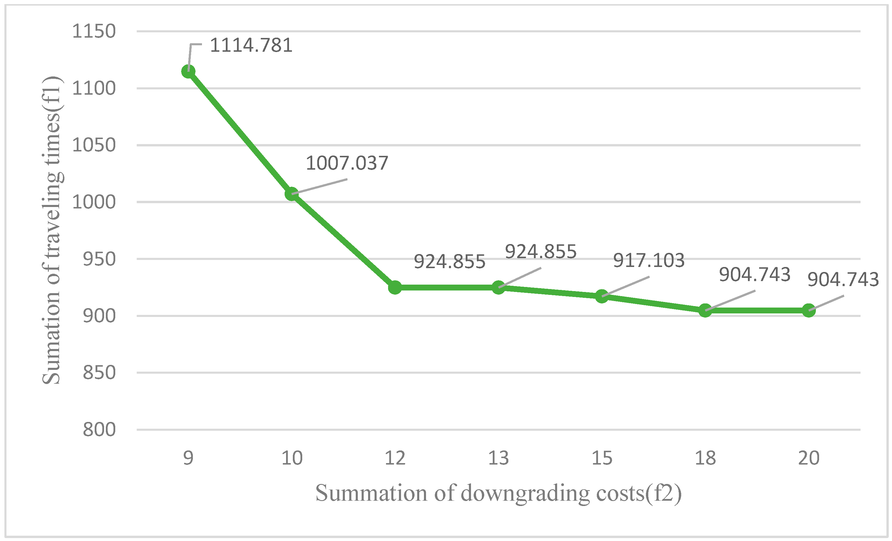
| Row Number | Epsilon Parameter | Optimal Solution Value |
|---|---|---|
| #1 | 9 | 1114.781 |
| #2 | 10 | 1007.037 |
| #3 | 12 | 924.855 |
| #4 | 13 | 924.855 |
| #5 | 15 | 917.103 |
| #6 | 18 | 904.743 |
| #7 | 20 | 904.743 |
| Row Number | Epsilon Parameter | Actual Used Downgrading Cost |
|---|---|---|
| #1 | 10 | 10 |
| #2 | 12 | 12 |
| #3 | 13 | 13 |
| #4 | 15 | 15 |
| #5 | 18 | 18 |
| #6 | 20 | 18 |
| #7 | 25 | 18 |
| #8 | 30 | 18 |
| #9 | 40 | 18 |
| #10 | 50 | 18 |
Publisher’s Note: MDPI stays neutral with regard to jurisdictional claims in published maps and institutional affiliations. |
© 2021 by the authors. Licensee MDPI, Basel, Switzerland. This article is an open access article distributed under the terms and conditions of the Creative Commons Attribution (CC BY) license (http://creativecommons.org/licenses/by/4.0/).
Share and Cite
Khodabandeh, P.; Kayvanfar, V.; Rafiee, M.; Werner, F. A Bi-Objective Home Health Care Routing and Scheduling Model with Considering Nurse Downgrading Costs. Int. J. Environ. Res. Public Health 2021, 18, 900. https://0-doi-org.brum.beds.ac.uk/10.3390/ijerph18030900
Khodabandeh P, Kayvanfar V, Rafiee M, Werner F. A Bi-Objective Home Health Care Routing and Scheduling Model with Considering Nurse Downgrading Costs. International Journal of Environmental Research and Public Health. 2021; 18(3):900. https://0-doi-org.brum.beds.ac.uk/10.3390/ijerph18030900
Chicago/Turabian StyleKhodabandeh, Pouria, Vahid Kayvanfar, Majid Rafiee, and Frank Werner. 2021. "A Bi-Objective Home Health Care Routing and Scheduling Model with Considering Nurse Downgrading Costs" International Journal of Environmental Research and Public Health 18, no. 3: 900. https://0-doi-org.brum.beds.ac.uk/10.3390/ijerph18030900