
The Spatial-Temporal Variation Characteristics of Natural Vegetation Drought in the Yangtze River Source Region, China

Abstract
:1. Introduction
2. Materials and Methods
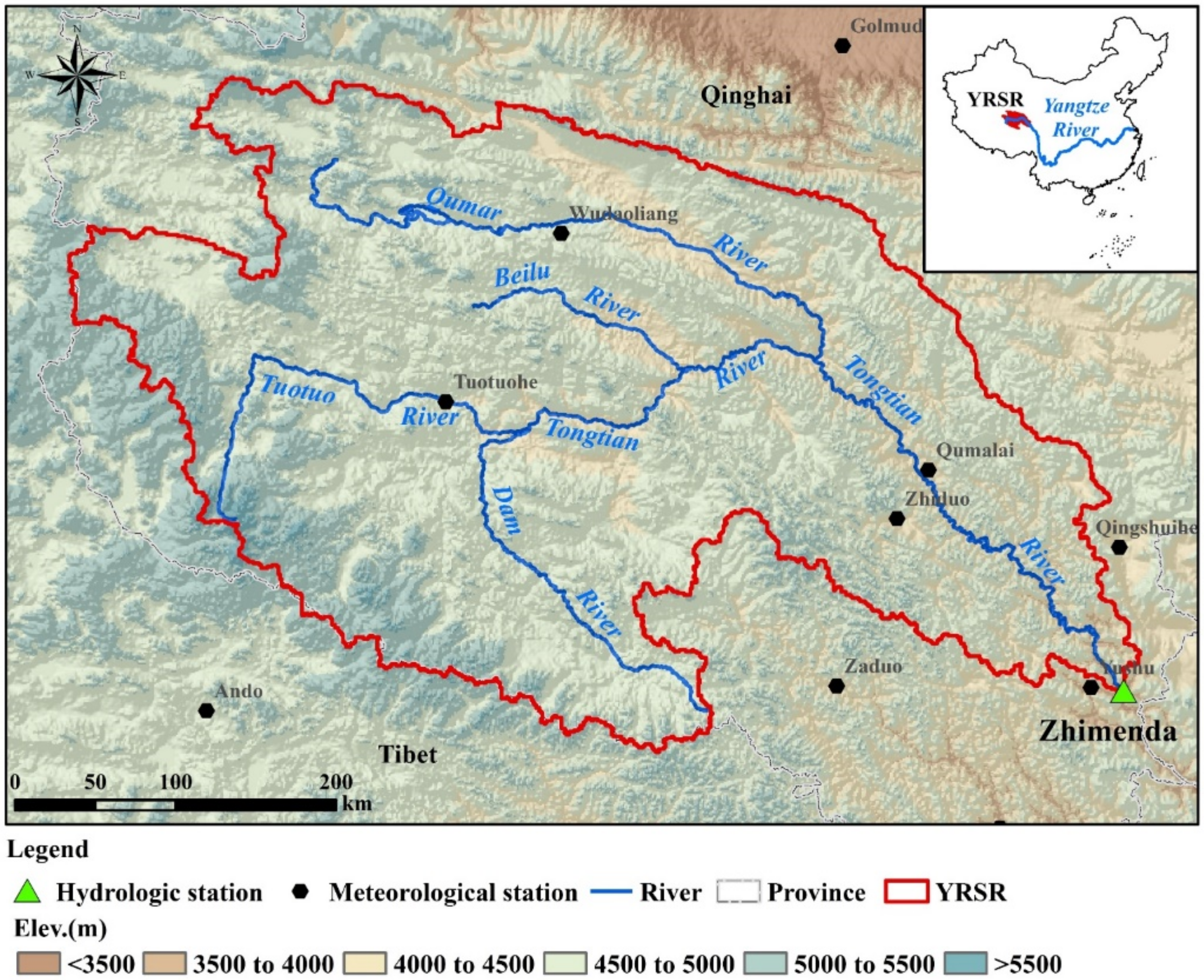
2.1. Study Area
2.2. Datasets
2.2.1. Hydro-Meteorological Data
2.2.2. Land Use/Land Cover Data
2.2.3. Soil Map and Soil Properties
2.2.4. Digital Elevation Model (DEM) Data
2.3. Methodology
2.3.1. Drought Index and Drought Identification
Standardized Water Supply-Demand Index (SSDI)
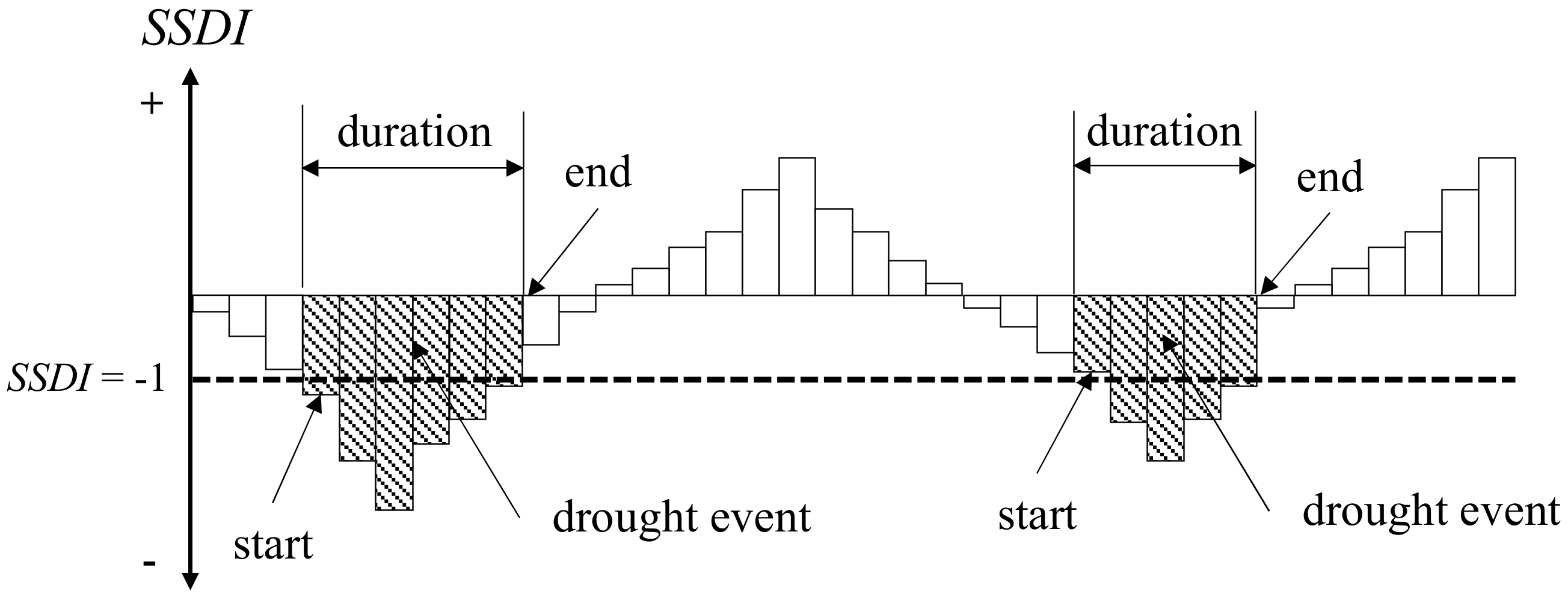
Drought Event Identification Based on Theory of Runs
- 1.
- Drought duration (DD) is defined as the time between the initiation and termination of a drought event, which is expressed in months in this study.where DDn refers to drought duration for the nth drought event. Tin and Ttn are initiation time and termination time, respectively.
- 2.
- Drought severity (DS) is the sum of SSDIs during the drought duration.where DSn refers to drought severity for the nth drought event.
- 3.
- Drought peak (DP) is the maximum absolute value of SSDIs of a drought event.where DPn refers to drought peak for the nth drought event. Tin and Ttn are initiation time and termination time, respectively.
- 4.
- Drought coverage area (DA) is the region affected by the drought, which is calculated as follows:where, DAn refers to the ratio of average drought affected area. A(i) is the area of region experiencing drought conditions. A is the area of the study region. In this research, the parameter A represents the area of grassland and forest ecosystem in the YRSR.
2.3.2. Trend Analysis for Drought Characteristic
Linear Regression Analysis
Mann–Kendall Test
2.3.3. Calculation of Bivariate Probability and Return Period via Copula Function
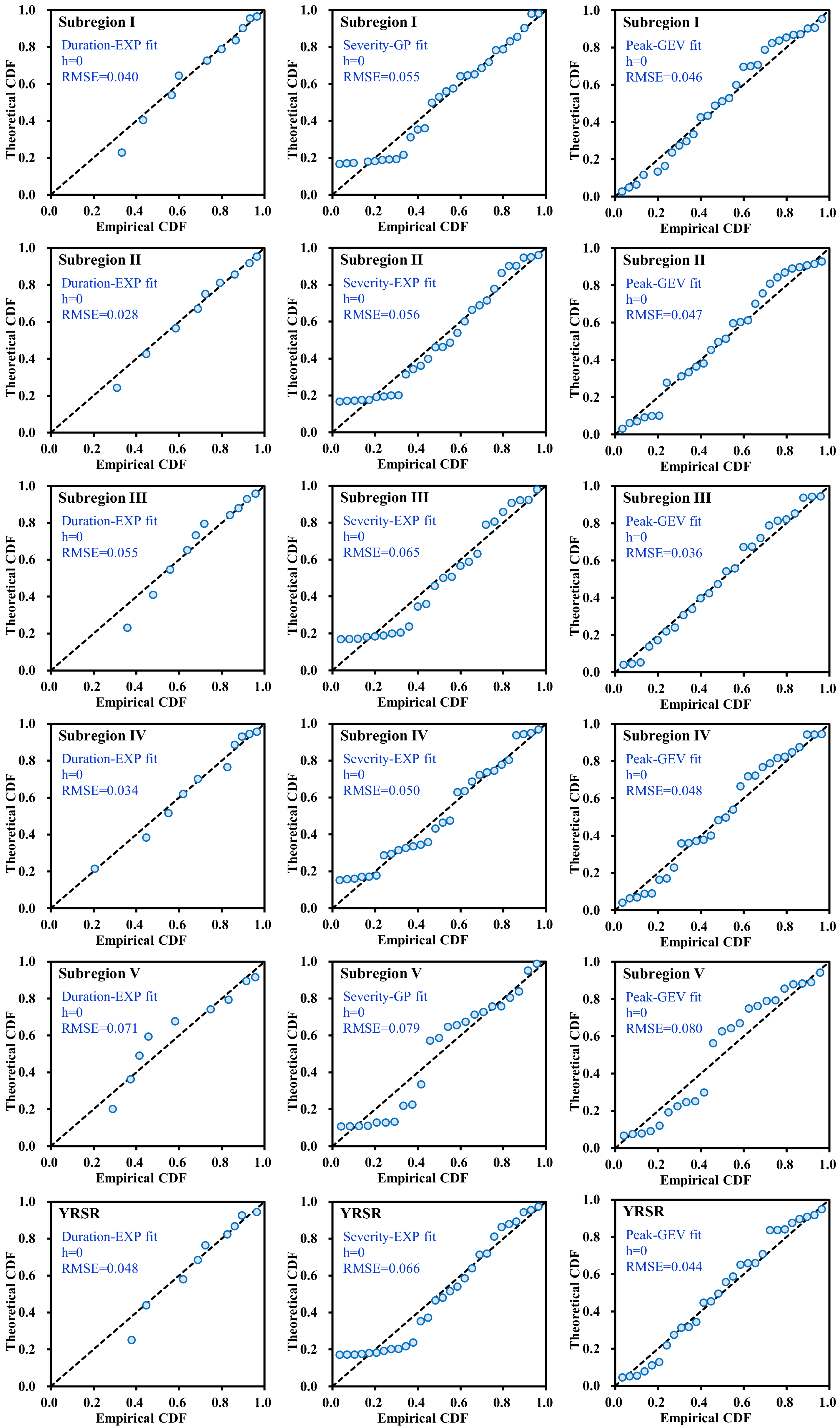
Selection of Marginal Distributions
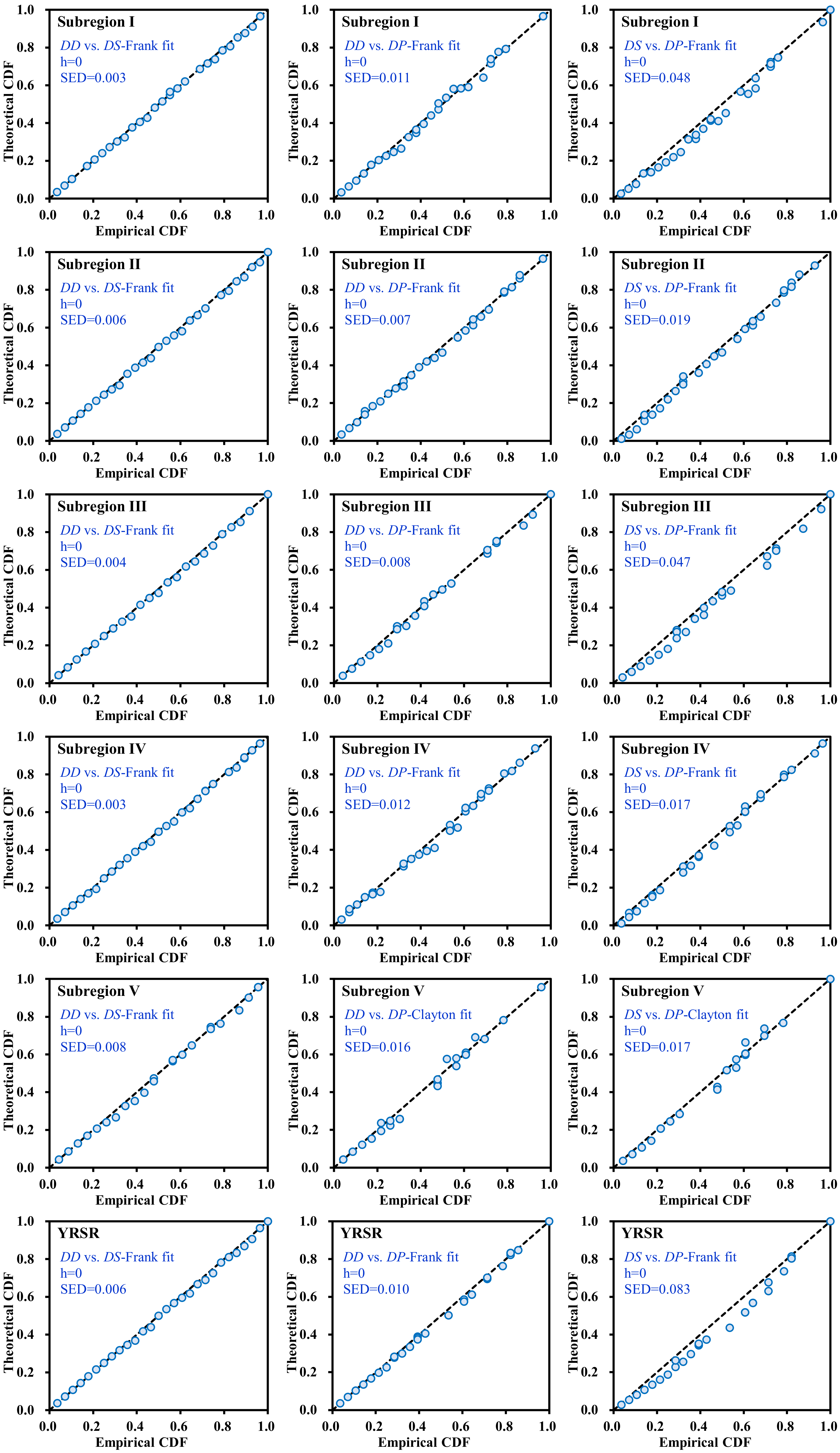
Selection of Copulas
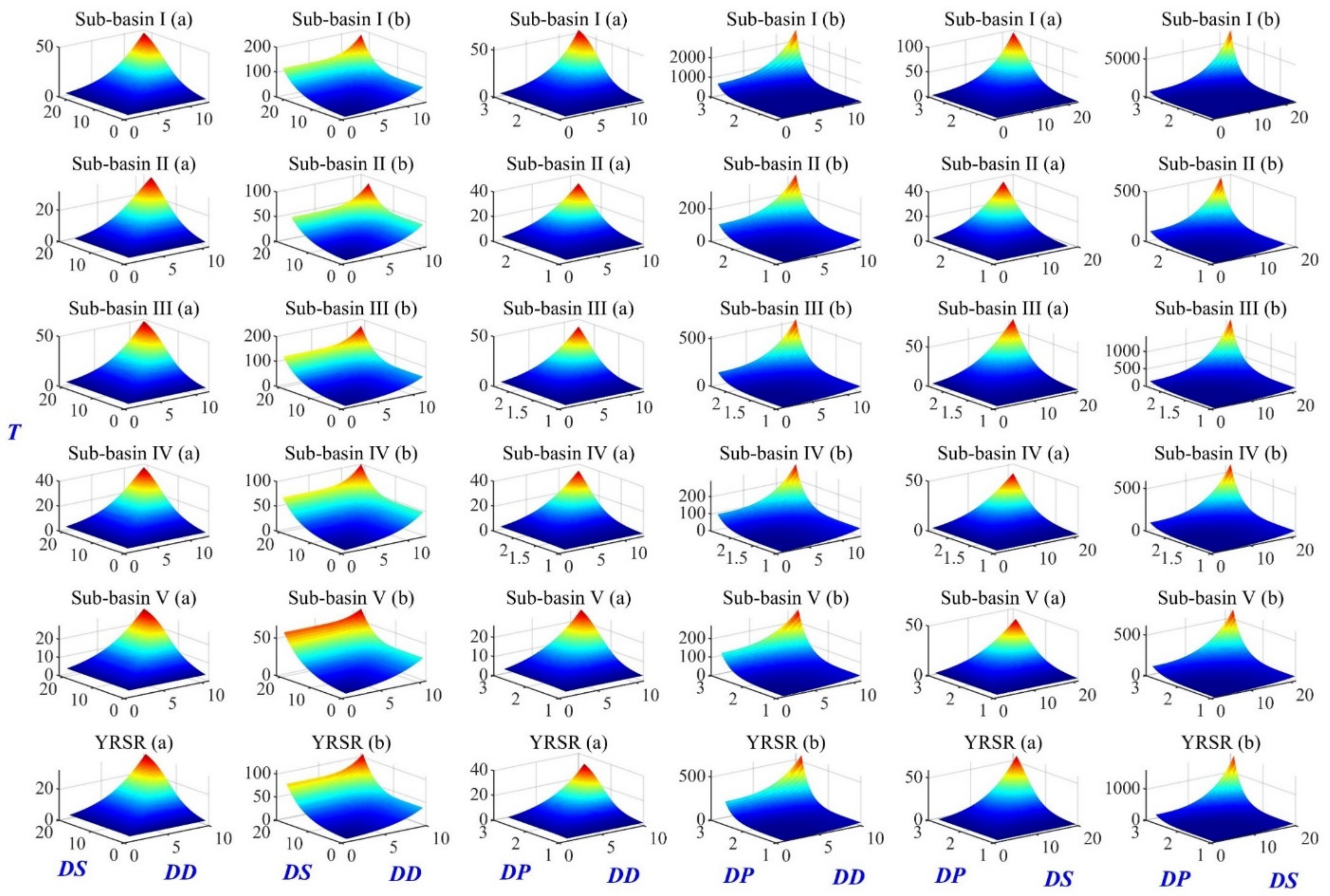
Bivariate Probability and Return Period
3. Results and Discussion
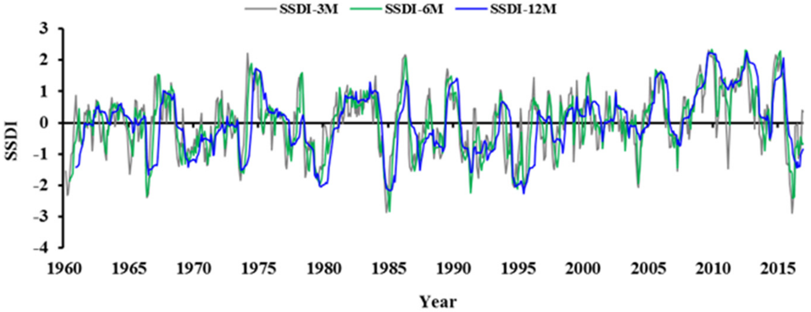
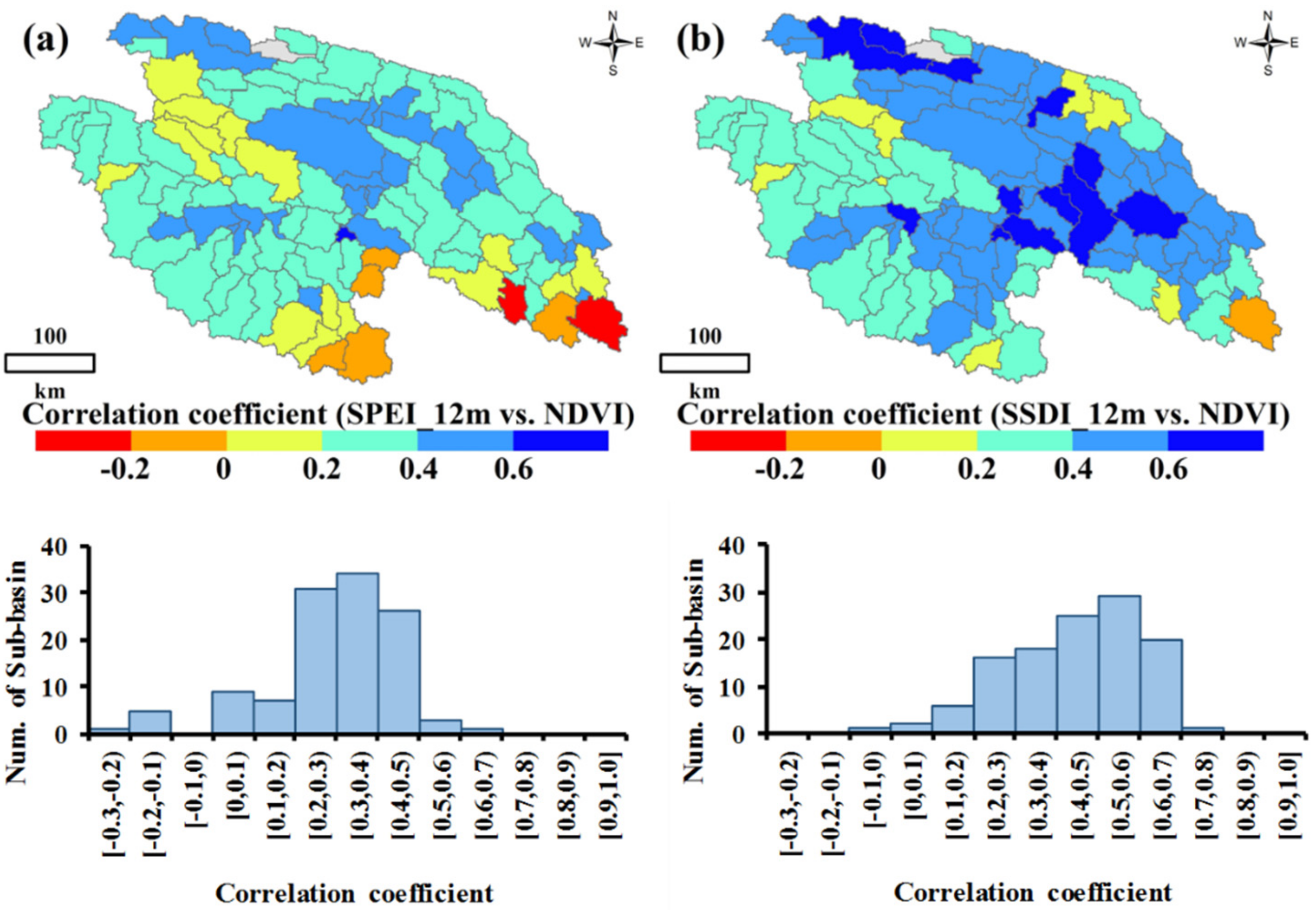
3.1. Time-Series Comparison of SSDI and SPEI with NDVI
3.2. Temporal and Spatial Variability of Drought Characteristics
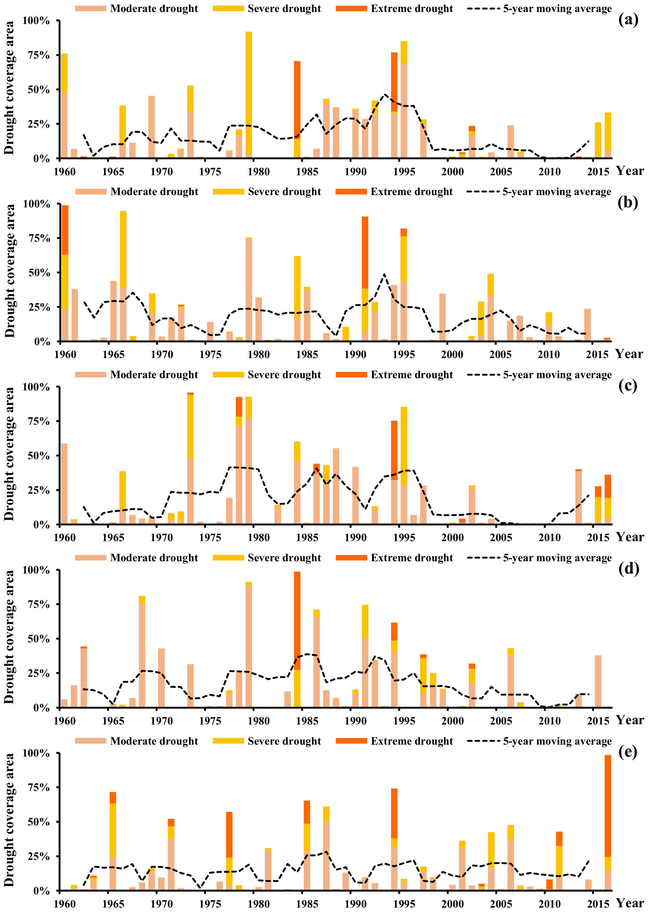
3.2.1. Temporal Variability of Droughts
3.2.2. Spatial Pattern of Drought Characteristics
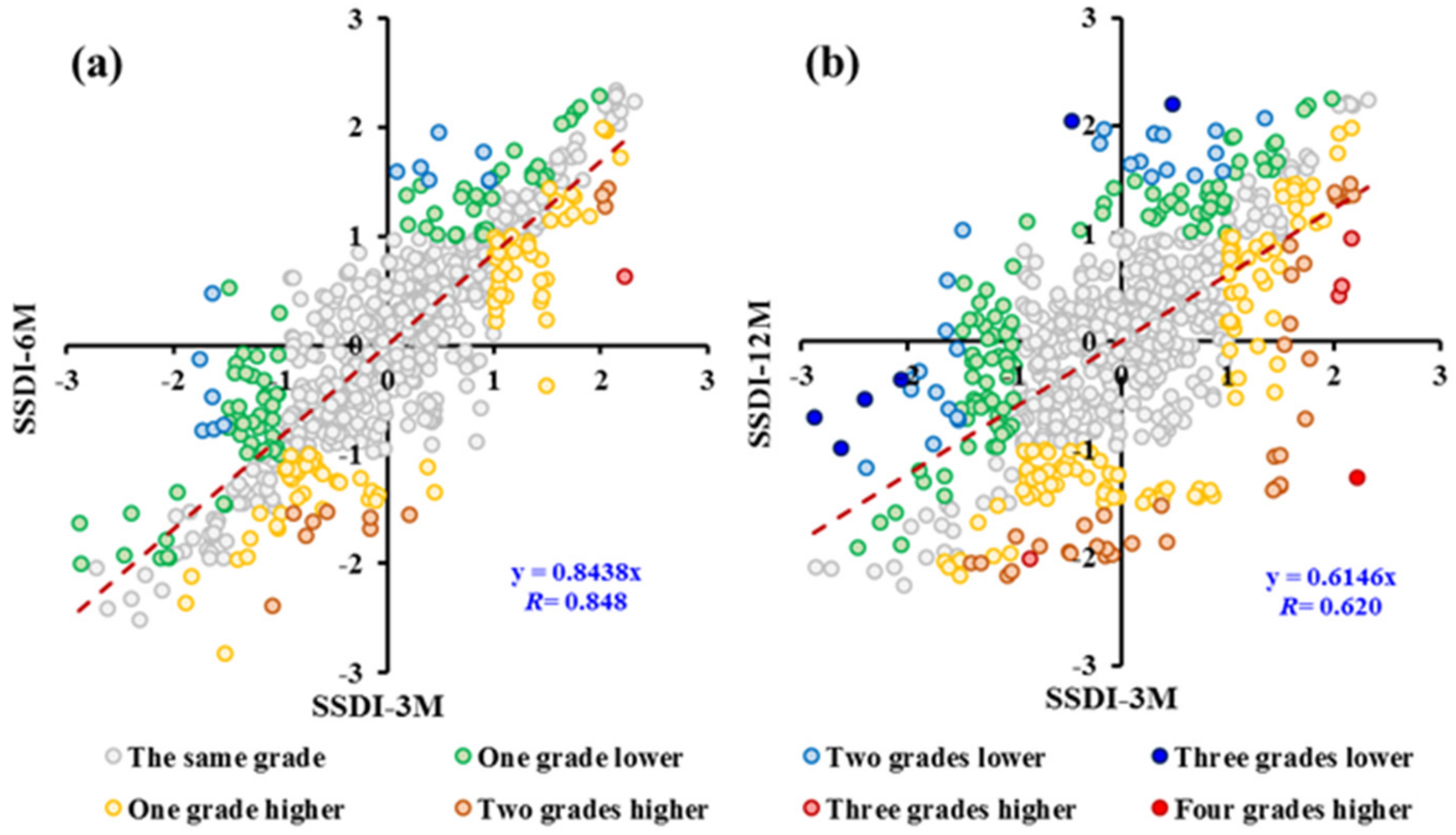
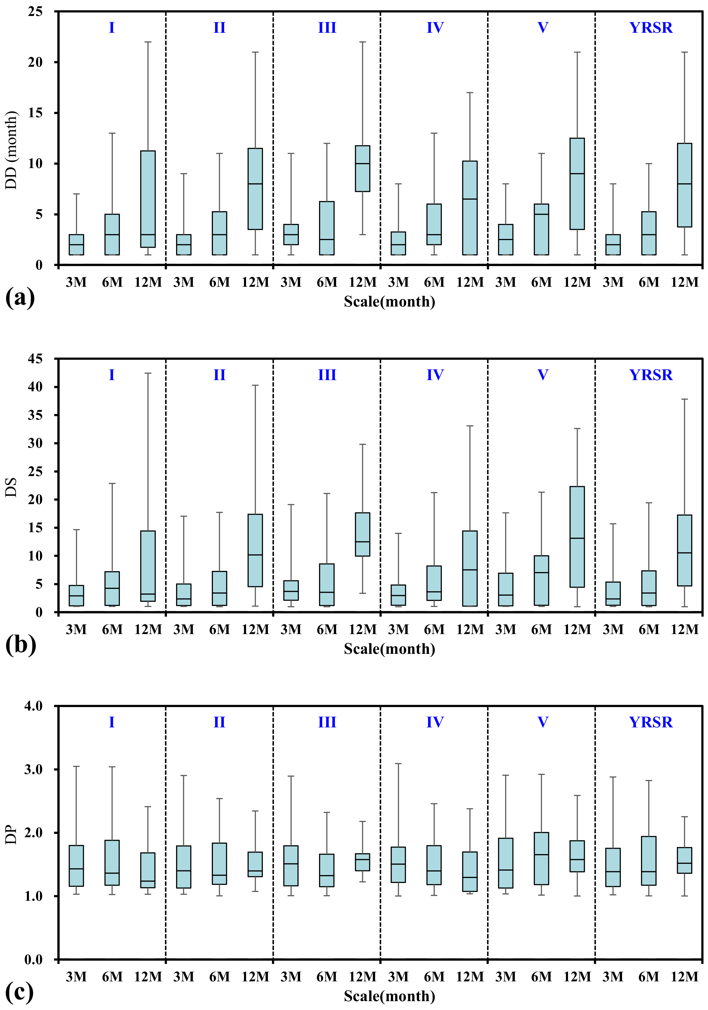
3.2.3. Effect of Time Scales on Drought Characteristics
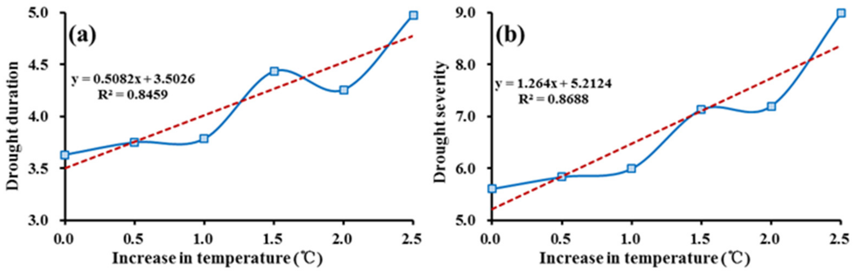
3.2.4. Sensitivity of Drought Characteristics to the Temperature
3.3. Regional Bivariate Probability and Return Period
3.3.1. Selection of the Marginal Distributions and Copulas
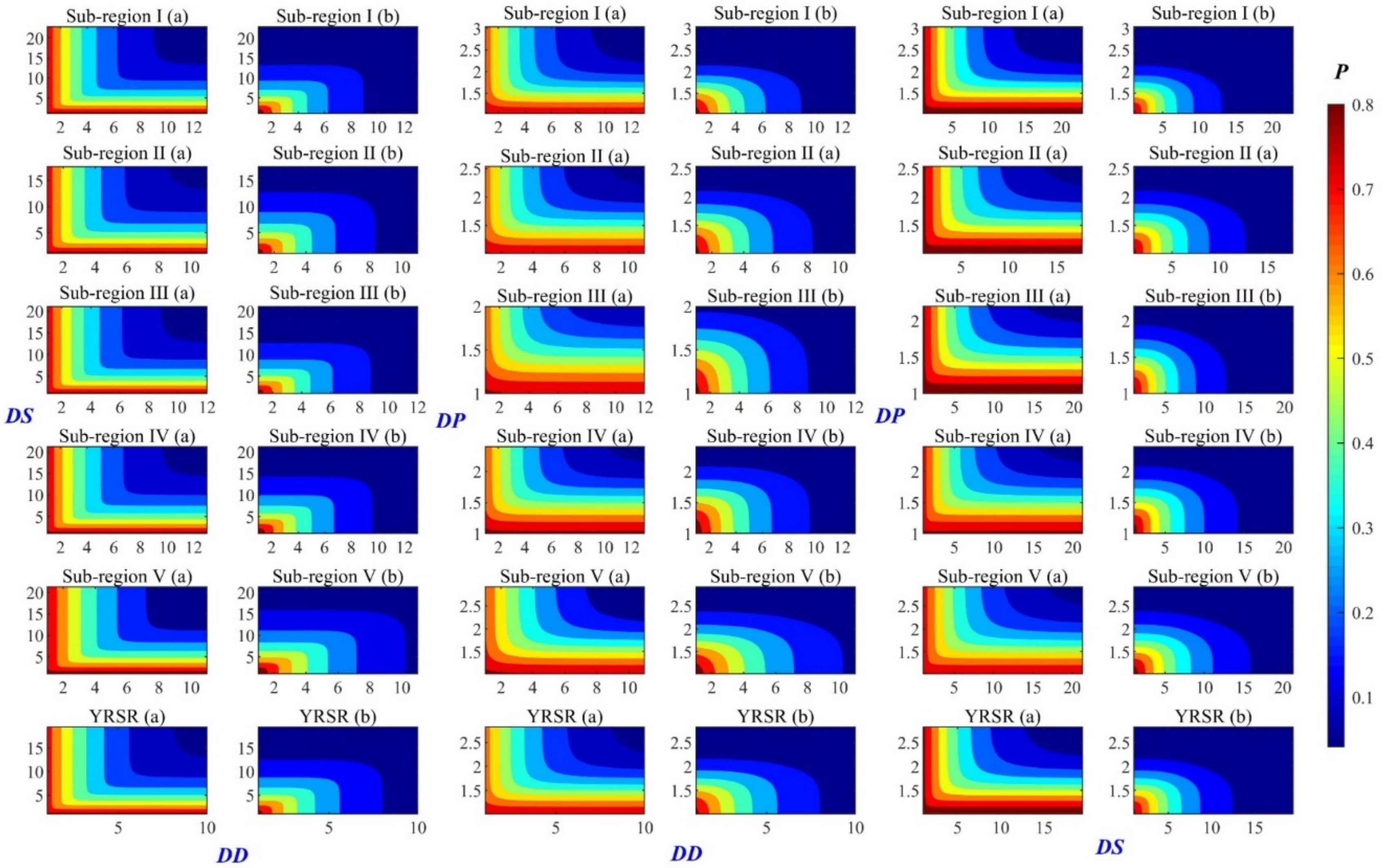
3.3.2. Regional Bivariate Probability of Drought Events
3.3.3. Bivariate Return Period of Drought Events
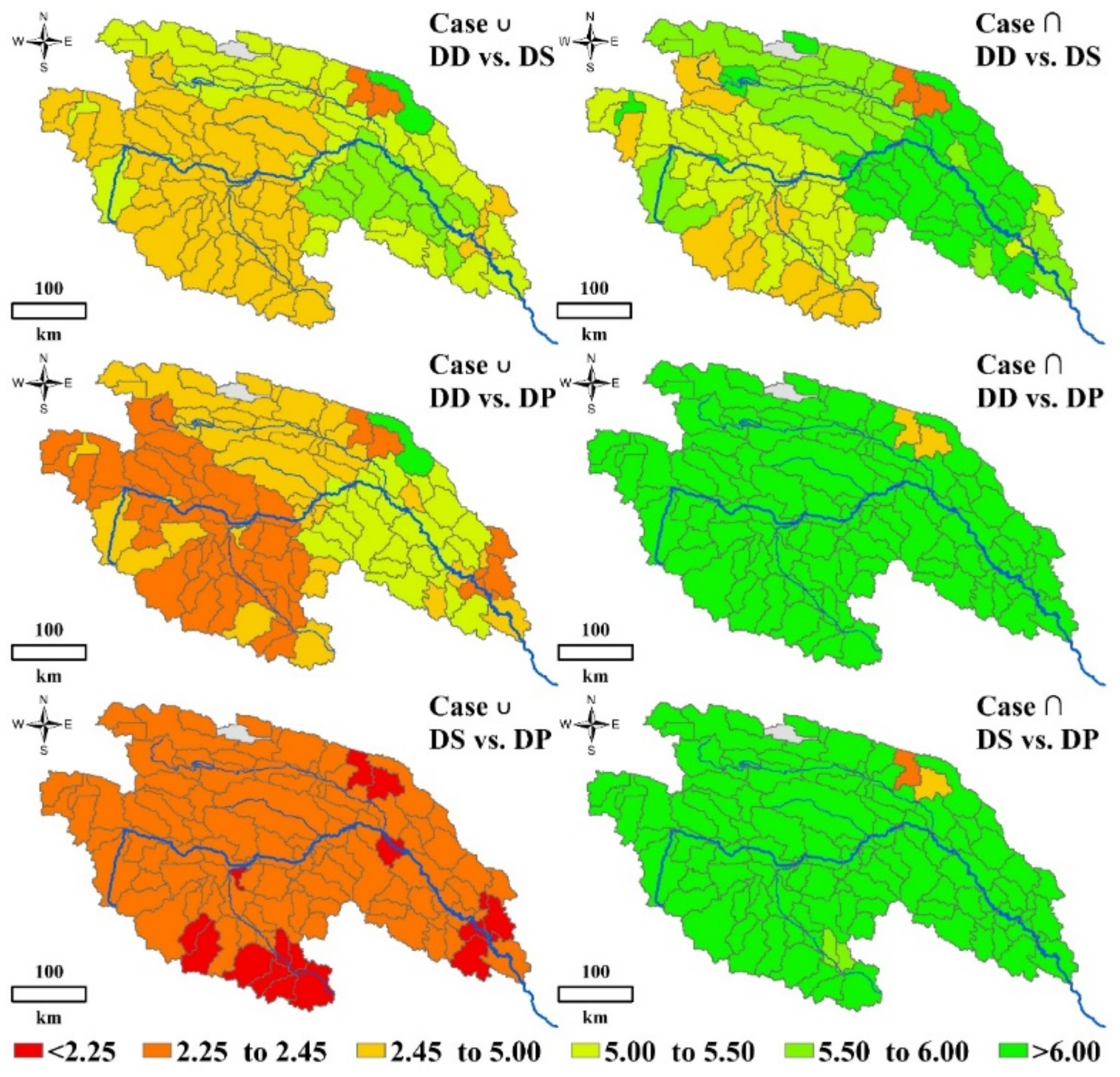
3.4. Spatial Distribution of Bivariate Probability and Return Period in the YRSR
4. Conclusions
- The time-series of SSDI and Standardized Precipitation and Evapotranspiration Drought Index (SPEI) with Normalized Difference Vegetation Index (NDVI) were compared in this study. There exists a higher correlation between constructed SSDI and NDVI. This result indicated that the constructed SSDI was reliable and can reflect the comprehensive characteristics of the ecological drought information more easily and effectively.
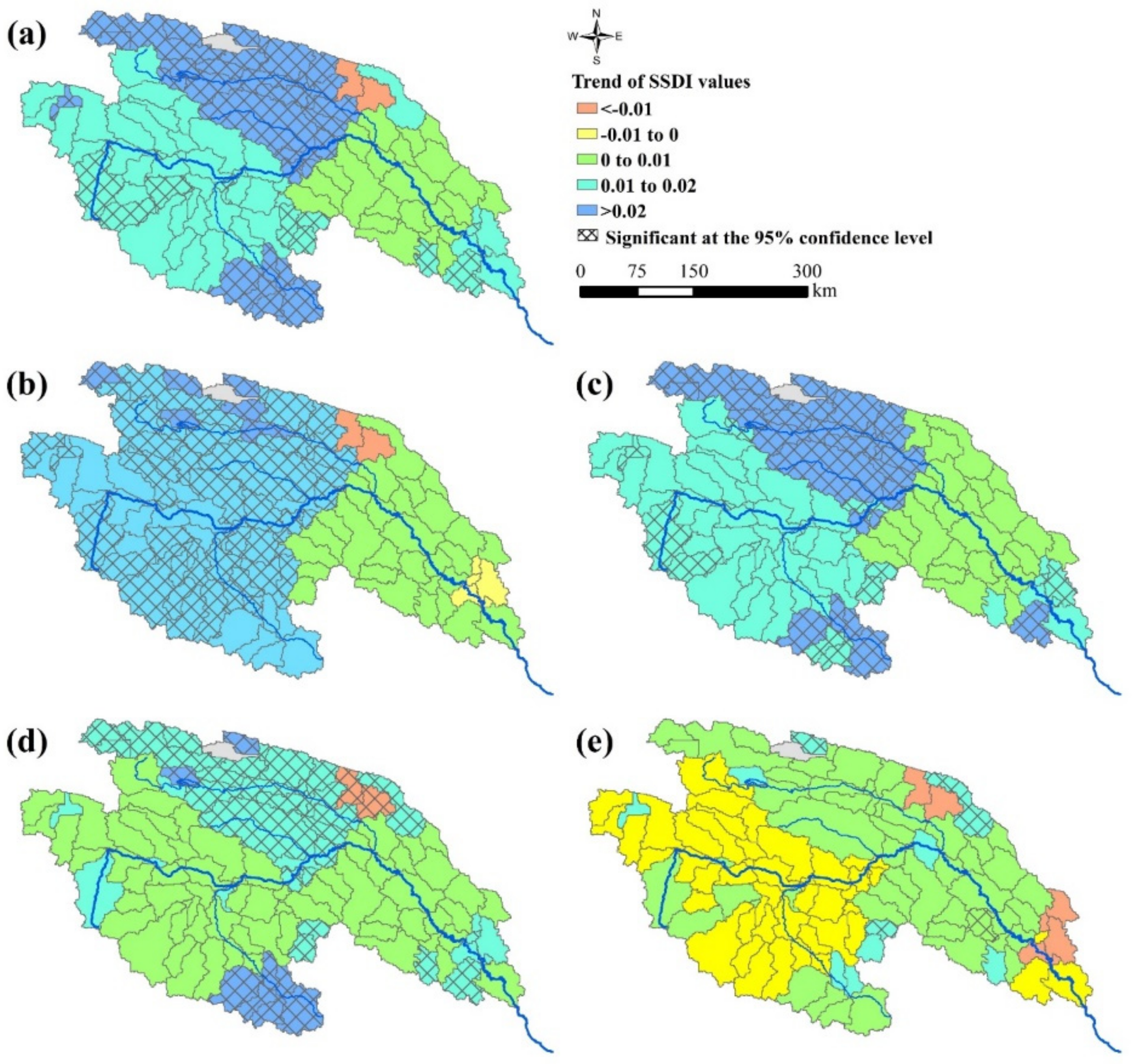
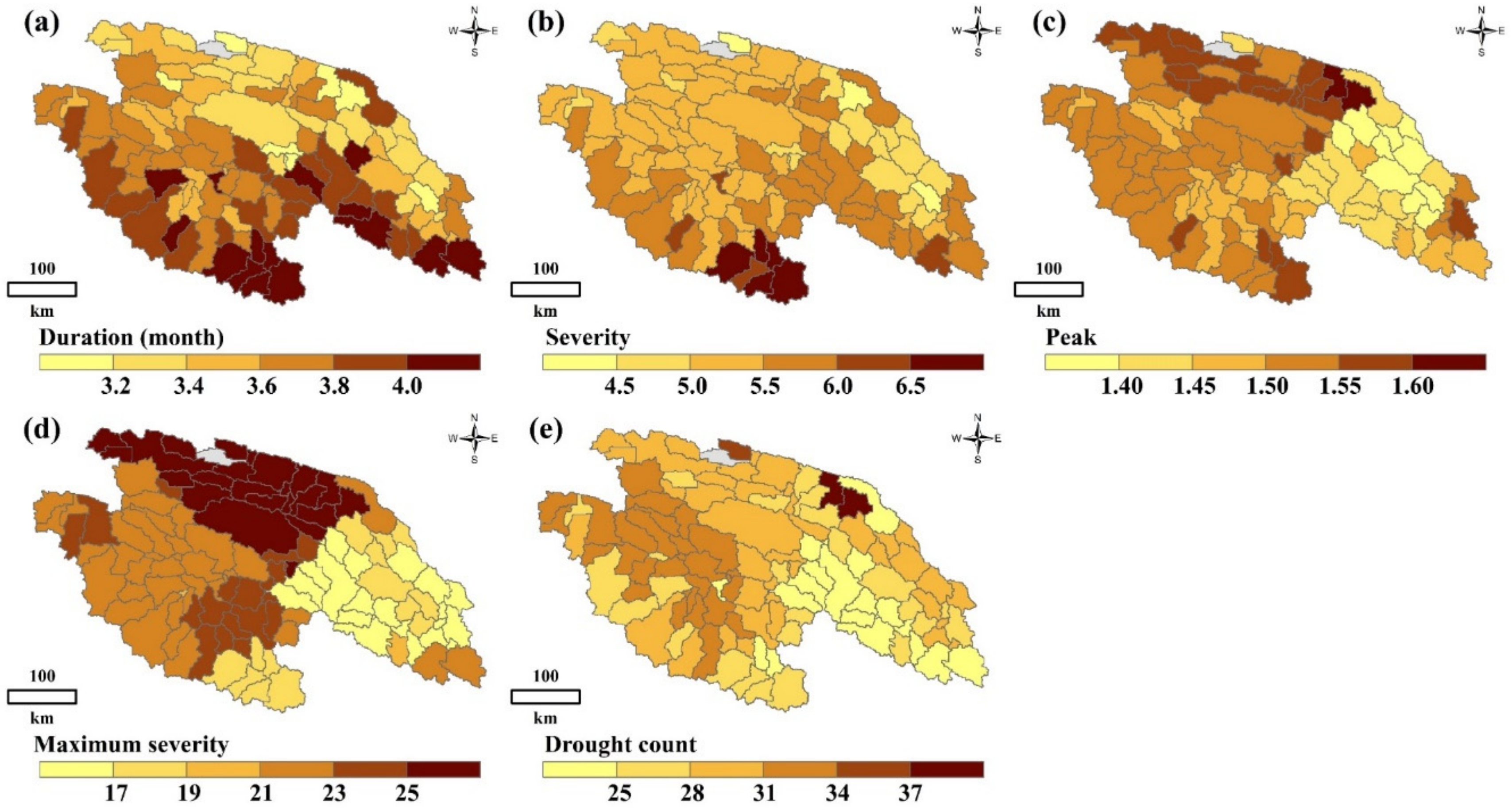
- The YRSR had witnessed the most severe drought episodes in the periods of late-1970s, mid-1980s and mid-1990s, but the SSDI showed a wetting trend since the mid-2000s, mainly because of a warmer and wetter climate in the most recent 10 years. However, the climate change has different effects on the dry condition at seasonal scales. The drought affected areas in spring, summer and autumn have decreased since 2000 while this area in winter has increased. The drought duration and severity showed a spatial variation among different regions in the YRSR. Generally, droughts in the Southern YRSR were relatively more severe with longer drought duration, implying that the Southern YRSR was an area that had been facing challenging drought conditions. The average drought duration and severity in the YRSR would be less susceptible to changes in temperature when the increase temperature was above 1.0 °C. However, the characteristics would be more susceptible to temperature in the YRSR when the increase temperature were above 1.0 °C. The average drought duration and severity is shown to increase by 20.7% and 32.6% with a 1 °C increase in temperature for the hypothetical scenarios with ΔT > 1 °C.
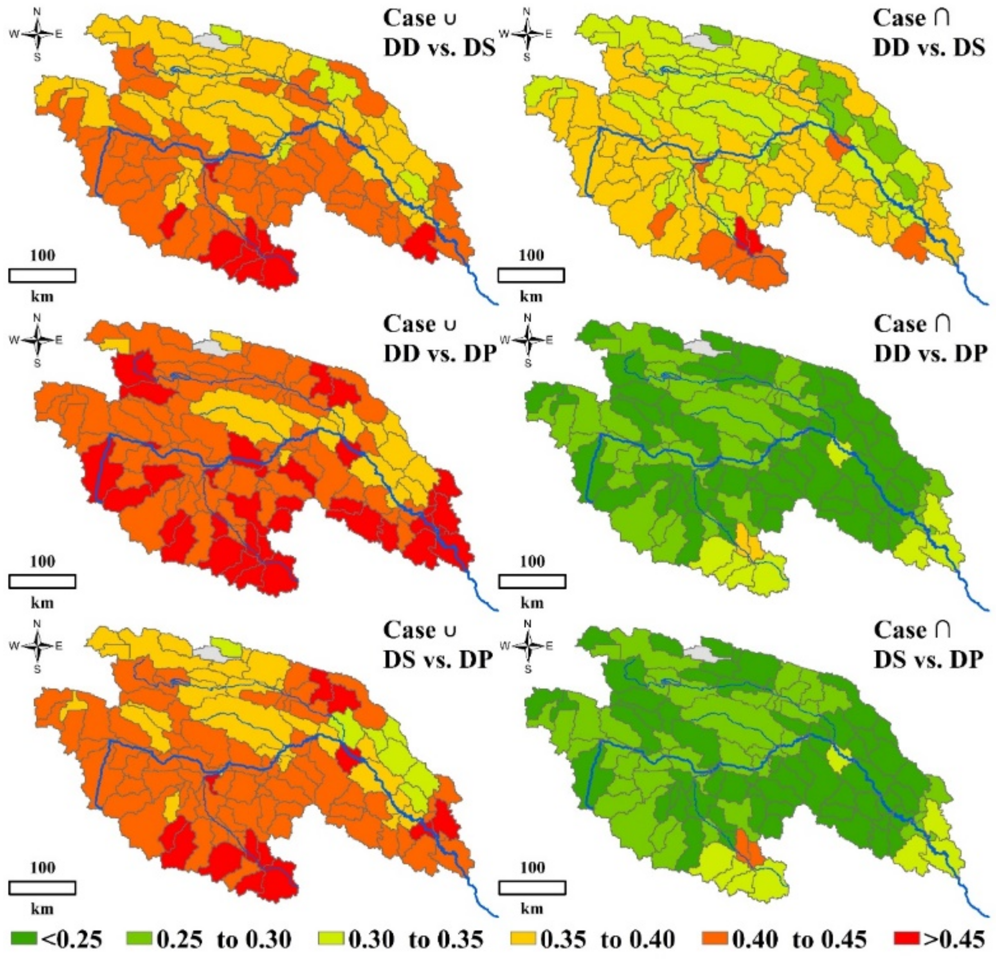
- The return periods of five sub-basins and the entire YRSR for case ‘‘∩” were longer than those in case ‘‘∪” and their spatial trends are highly consistent. High return periods were found in Qumar River Basin. While, low return periods were found in most areas of Togton River Basin and Dam River Basin, implying that severe ecological drought events occurred more frequently.
Author Contributions
Funding
Institutional Review Board Statement
Informed Consent Statement
Conflicts of Interest
References
- Touma, D.; Ashfaq, M.; Nayak, M.; Kao, S.-C.; Diffenbaugh, N. A multi-model and multi-index evaluation of drought characteristics in the 21st century. J. Hydrol. 2015, 526, 196–207. [Google Scholar] [CrossRef] [Green Version]
- Vicca, S.; Balzarolo, M.; Filella, I.; Granier, A.; Herbst, M.; Knohl, A.; Longdoz, B.; Mund, M.; Nagy, Z.; Pintér, K.; et al. Remotely-sensed detection of effects of extreme droughts on gross primary production. Sci. Rep. 2016, 6, 28269. [Google Scholar] [CrossRef]
- Schwalm, C.R.; Anderegg, W.R.L.; Michalak, A.M.; Fisher, J.B.; Biondi, F.; Koch, G.; Litvak, M.; Ogle, K.; Shaw, J.D.; Wolf, A.; et al. Global patterns of drought recovery. Nature 2017, 548, 202–205. [Google Scholar] [CrossRef]
- Du, L.; Mikle, N.; Zou, Z.; Huang, Y.; Shi, Z.; Jiang, L.; McCarthy, H.R.; Lou, Y. Global patterns of extreme drought-induced loss in land primary production: Identifying ecological extremes from rain-use efficiency. Sci. Total Environ. 2018, 628–629, 611–620. [Google Scholar] [CrossRef]
- Lesk, C.; Rowhani, P.; Ramankutty, N. Influence of extreme weather disasters on global crop production. Nature 2016, 529, 84–87. [Google Scholar] [CrossRef]
- United Nations International Strategy for Disaster Reduction Secretariat. Global Assessment Report on Disaster Risk Reduction. In Risk and Poverty in a Changing Climate, Invest Today for a Safer Tomorrow; UN, International Strategy for Disaster Reduction: Geneva, Switzerland, 2009. [Google Scholar]
- Stocker, T.F.; Qin, D.; Plattner, G.K.; Tignor, M.M.B.; Allen, S.K.; Boschung, J.; Nauels, A.; Xia, Y.; Bex, V.; Midgley, P.M. Climate Change 2013: The physical Science Basis. In Contribution of Working Group I to the Fifth Assessment Report of the Intergovernmental Panel on Climate Change; Cambridge University Press: Cambridge, UK, 2013. [Google Scholar]
- World Meteorological Organization. Drought and Agriculture. World Meteorological Organization; Technical Note 138; WMO Publication: Geneva, Switzerland, 1975. [Google Scholar]
- Mishra, A.K.; Singh, V.P. A review of drought concepts. J. Hydrol. 2010, 391, 202–216. [Google Scholar] [CrossRef]
- McKee, T.B.; Doesken, N.J.; Kleist, J. The Relationship of Drought Frequency and Duration to Time Scales. In Proceedings of the 8th Conference on Applied Climatology, Anaheim, CA, USA, 7–22 January 1993. [Google Scholar]
- McKee, T.B.; Doesken, N.J.; Kleist, J. Drought Monitoring with Multiple Time Scales. In Proceedings of the 9th Conference on Applied Climatology, Dallas, TX, USA, 15–20 January 1995. [Google Scholar]
- Serrano, S.M.V.; Beguería, S.; Moreno, J.I.L. A multiscalar drought index sensitive to global warming: The standardized precipitation evapotranspiration index. J. Clim. 2010, 23, 1696–1718. [Google Scholar] [CrossRef] [Green Version]
- Palmer, W.C. Meteorologic Drought. In Research Paper No. 45; US Department of Commerce Weather Bureau: Washington, DC, USA, 1965. [Google Scholar]
- Hollinger, S.E.; Isard, S.A.; Welford, M.R. A New Soil Moisture Drought Index for Predicting Crop Yields. In Applied Climatology; American Meteor Society: Anaheim, CA, USA, 1993. [Google Scholar]
- Yevjevich, V. An Objective Approach to Definitions and Investigations of Continental Hydrologic Droughts. In Hydrology Papers 23; Colorado State University Publication: Fort Collins, CO, USA, 1967. [Google Scholar]
- Loaiciga, H.A.; Leipnik, R.B. Stochastic renewal model of low-flow streamflow sequences. Stoch. Hydrol. Hydraul. 1996, 10, 65–85. [Google Scholar] [CrossRef]
- Chung, C.H.; Salas, J.D. Drought occurrences probabilities and risks of dependent hydrologic processes. J. Hydrol. Eng. 2000, 5, 259–268. [Google Scholar] [CrossRef]
- Salas, J.D.; Fu, C.; Cancelliere, A.; Dustin, D.; Bode, D.; Pineda, A.; Vincent, E. Characterizing the severity and risk of drought in the Poudre River. Colorado. J. Water Resour. Plan. Manag. 2005, 131, 383–393. [Google Scholar] [CrossRef]
- Mishra, A.K.; Desai, V.R.; Singh, V.P. Drought forecasting using a hybrid stochastic and neural network model. J. Hydrol. Eng. 2007, 12, 626–638. [Google Scholar] [CrossRef]
- Serinaldi, F.; Bonaccorso, B.; Cancelliere, A.; Grimaldi, S. Probabilistic characterization of drought properties through copulas. Phys. Chem. Earth 2009, 34, 596–605. [Google Scholar] [CrossRef]
- Jiang, R.; Xie, J.; He, H.; Luo, J.; Zhu, J. Use of four drought indices for evaluating drought characteristics under climate change in Shaanxi, China: 1951-2012. Nat. Hazards 2015, 75, 2885–2903. [Google Scholar] [CrossRef]
- Zargar, A.; Sadiq, R.; Naser, B.; Khan, F.I. A review of drought indices. Environ. Rev. 2011, 19, 333–349. [Google Scholar] [CrossRef]
- Kogan, F.N. Remote sensing of weather impacts on vegetation in non-homogeneous areas. Int. J. Remote Sens. 1990, 11, 1405–1419. [Google Scholar] [CrossRef]
- Weng, B.; Yan, D.; Wang, H.; Liu, J.; Yang, Z.; Qin, T.; Yin, J. Drought assessment in the Dongliao River basin: Traditional approaches vs. generalized drought assessment index based on water resources systems. Nat. Hazards Earth Syst. Sci. 2015, 15, 1889–1906. [Google Scholar] [CrossRef] [Green Version]
- Yao, Z.; Liu, Z.; Huang, H.; Liu, G.; Wu, S. Statistical estimation of the impacts of glaciers and climate change on river runoff in the headwaters of the Yangtze River. Quat. Int. 2014, 336, 89–97. [Google Scholar] [CrossRef]
- Wang, R.; Yao, Z.; Liu, Z.; Wu, S.; Jiang, L.; Wang, L. Snow cover variability and snowmelt in a high-altitude ungauged catchment. Hydrol. Process. 2015, 29, 3665–3676. [Google Scholar] [CrossRef]
- Du, Y.; Berndtsson, R.; An, D.; Zhang, L.; Hao, Z.; Yuan, F. Hydrologic Response of Climate Change in the Source Region of the Yangtze River, Based on Water Balance Analysis. Water 2017, 9, 115. [Google Scholar] [CrossRef] [Green Version]
- Yuan, Z.; Xu, J.; Wang, Y. Historical and future changes of blue water and green water resources in the Yangtze River source region, China. Theor. Appl. Climatol. 2019, 138, 1035–1047. [Google Scholar] [CrossRef]
- Chen, J. Water cycle mechanism in the source region of Yangtze River. J. Yangtze River Sci. Res. Inst. 2013, 30, 1–5. [Google Scholar]
- Yuan, Z.; Xu, J.; Chen, J.; Huo, J.; Yu, Y.; Locher, P.; Xu, B. Drought assessment and projection under climate change: A case study in the middle and lower Jinsha River Basin. Adv. Meteorol. 2017, 5757238. [Google Scholar] [CrossRef] [Green Version]
- Schuol, J.; Abbaspour, K.C.; Yang, H. Modeling blue and green water availability in Africa. Water Resour. Res. 2008, 44, 212–221. [Google Scholar] [CrossRef] [Green Version]
- Zhang, W.; Zha, X.; Li, J.; Liang, W.; Ma, Y.; Fan, D.; Li, S. Spatialtemporal change of blue water and green water resources in the headwater of Yellow River Basin, China. Water Resour. Manag. 2014, 28, 4715–4732. [Google Scholar] [CrossRef]
- Abbaspour, K.C.; Rouholahnejad, E.; Vaghefi, S.; Srinivasan, R.; Yang, H.; Kløve, B. A continental-scale hydrology and water quality model for Europe: Calibration and uncertainty of a high-resolution large-scale SWAT model. J. Hydrol. 2015, 524, 733–752. [Google Scholar] [CrossRef] [Green Version]
- Zhao, F.; Li, H.; Li, C.; Cai, Y.; Wang, X.; Liu, Q. Analyzing the influence of landscape pattern change on ecological water requirements in an arid/semiarid region of China. J. Hydrol. 2019, 578, 124098. [Google Scholar] [CrossRef]
- Ahmad, M.I.; Sinclair, C.D.; Werritty, A. Log-logistic flood frequency analysis. J. Hydrol. 1988, 98, 205–224. [Google Scholar] [CrossRef]
- Yin, J.; Yan, D.; Yang, Z.; Yuan, Z.; Yuan, Y.; Wang, H.; Shi, X. Research on Historical and Future Spatial-Temporal Variability of Precipitation in China. Adv. Meteorol. 2016, 2016, 9137201. [Google Scholar] [CrossRef]
- Tabari, H.; Talaee, P.H.; Ezani, A.; Some’e, B. Shift changes andmonotonic trends in autocorrelated temperature series over Iran. Theor. Appl. Climatol. 2012, 109, 95–108. [Google Scholar] [CrossRef]
- Shiau, J.T. Fitting drought duration and severity with two-dimensional copulas. Water Resour. Manag. 2006, 20, 795–815. [Google Scholar] [CrossRef]
- Ayantobo, O.O.; Li, Y.; Song, S.; Javed, T.; Yao, N. Probabilistic modelling of drought events in China via 2-dimensional joint copula. J. Hydrol. 2018, 559, 373–391. [Google Scholar] [CrossRef]
- Guo, Y.; Huang, S.; Huang, Q.; Wang, H.; Wang, L.; Fang, W. Copulas-based bivariate socioeconomic drought dynamic risk assessment in a changing environment. J. Hydrol. 2019, 575, 1052–1064. [Google Scholar] [CrossRef]
- Gringorten, I.I. A plotting rule for extreme probability paper. J. Geophys. Res. 1963, 68, 813–814. [Google Scholar] [CrossRef]
- Weng, B.; Zhang, P.; Li, S. Drought risk assessment in China with different spatial scales. Arab. J. Geosci. 2015, 8, 10193–10202. [Google Scholar] [CrossRef]
- Genest, C.; MacKay, J. The joy of copulas: Bivariate distributions with uniform marginals. Am. Stat. 1986, 40, 280–283. [Google Scholar]
- Wang, R.; Zhao, C.; Zhang, J.; Guo, E.; Li, D.; Alu, S.; Ha, S.; Dong, Z. Bivariate copula function-based spatial-temporal characteristics analysis of drought in Anhui Province, China. Meteorol. Atmos. Phys. 2019, 131, 1341–1355. [Google Scholar] [CrossRef]
- Ribeiro, A.F.; Russo, A.; Gouveia, C.M.; Páscoa, P. Copula-based agricultural drought risk of rainfed cropping systems. Agric. Water Manag. 2019, 223, 105689. [Google Scholar] [CrossRef]
- Nelsen, R.B. An Introduction to Copulas. In Statistics; Springer: New York, NY, USA, 2006. [Google Scholar]
- McVicar, T.R.; Jupp, D.L.B. The current and potential operational uses of remote sensing to aid decisions on drought exceptional circumstances in Australia: A review. Agric. Syst. 1998, 57, 399–468. [Google Scholar] [CrossRef]
- Liu, J.; Chen, J.; Xu, J.; Lin, Y.; Yuan, Z.; Zhou, M. Attribution of Runoff Variation in the Headwaters of the Yangtze River Based on the Budyko Hypothesis. Int. J. Environ. Res. Public Health 2019, 16, 2506. [Google Scholar] [CrossRef] [Green Version]
- Kang, S.; Zhang, Y.; Qin, D.; Ren, J.; Zhang, Q.; Grigholm, B.; Mayewski, P.A. Recent temperature increase recorded in an ice core in the source region of Yangtze River. Chin. Sci. Bull. 2007, 52, 825–831. [Google Scholar] [CrossRef]
- Chongyi, E.; Hu, H.; Xie, H.; Sun, Y. Temperature change and its elevation dependency in the source region of the Yangtze River and Yellow River. J. Geogr. Geol. 2014, 6, 124–131. [Google Scholar]
- Piao, S.; Fang, J.; Zhou, L.; Ciais, P.; Zhu, B. Variations in satellite-derived phenology in China’s temperate vegetation. Glob. Chang. Biol. 2006, 12, 672–685. [Google Scholar] [CrossRef]
- Ding, M.; Zhang, Y.; Sun, X.; Liu, L.; Wang, Z.; Bai, W. Spatialtemporal variation in alpine grassland phenology in the Qinghai-Tibetan Plateau from 1999 to 2009. Chin. Sci. Bull. 2013, 58, 396–405. [Google Scholar] [CrossRef] [Green Version]
- Wang, S.; Zhang, B.; Yang, Q.; Chen, G.; Yang, B.; Lu, L.; Shen, M.; Peng, Y. Responses of net primary productivity to phenological dynamics in the Tibetan Plateau, China. Agric. For. Meteorol. 2017, 232, 235–246. [Google Scholar] [CrossRef]


| Drought Grade | Range of SSDI Value |
|---|---|
| Near normal | 1.00 > SSDI > −1.00 |
| Moderate drought | −1.00 ≥ SSDI > −1.50 |
| Severe drought | −1.50 ≥ SSDI > −2.00 |
| Extreme drought | −2.00 ≥ SSDI |
| Subregion | DD vs. DS | DD vs. DP | DS vs. DP | |||
|---|---|---|---|---|---|---|
| Copula | Parameter (θ) | Copula | Parameter (θ) | Copula | Parameter (θ) | |
| I | Frank | 33.094 | Frank | 8.192 | Frank | 10.202 |
| II | Frank | 25.537 | Frank | 9.184 | Frank | 11.220 |
| III | Frank | 31.090 | Frank | 7.205 | Frank | 8.897 |
| IV | Frank | 32.708 | Frank | 9.804 | Frank | 11.906 |
| V | Frank | 18.411 | Clayton | 2.042 | Clayton | 3.509 |
| YRSR | Frank | 27.058 | Frank | 9.024 | Frank | 10.889 |
| Region | T | DD | DS | DP | DD vs. DS Return Period | DD vs. DP Return Period | DS vs. DP Return Period | |||
|---|---|---|---|---|---|---|---|---|---|---|
| Case∪ | Case ∩ | Case∪ | Case ∩ | Case∪ | Case ∩ | |||||
| Subregion I | 5 | 3.6 | 5.3 | 0.2 | 4.7 | 5.3 | 4.1 | 6.3 | 4.3 | 6.0 |
| 10 | 6.3 | 9.2 | 0.6 | 9.0 | 11.2 | 7.3 | 15.7 | 7.6 | 14.5 | |
| 20 | 9.0 | 13.2 | 1.0 | 16.5 | 25.4 | 12.9 | 44.1 | 13.4 | 39.2 | |
| 50 | 12.5 | 18.4 | 2.0 | 35.1 | 87.1 | 28.5 | 204.2 | 29.2 | 173.7 | |
| 100 | 15.2 | 22.3 | 3.1 | 62.3 | 253.9 | 53.7 | 719.7 | 54.6 | 598.3 | |
| Subregion II | 5 | 3.2 | 4.9 | 0.2 | 4.7 | 5.4 | 4.2 | 6.1 | 4.3 | 5.9 |
| 10 | 5.7 | 8.7 | 0.5 | 8.8 | 11.5 | 7.5 | 14.9 | 7.8 | 13.9 | |
| 20 | 8.2 | 12.6 | 1.0 | 16.0 | 26.7 | 13.3 | 40.6 | 13.7 | 36.7 | |
| 50 | 11.5 | 17.6 | 1.9 | 33.8 | 96.1 | 29.0 | 182.6 | 29.7 | 158.2 | |
| 100 | 14.0 | 21.4 | 3.0 | 60.4 | 289.5 | 54.3 | 633.5 | 55.1 | 536.3 | |
| Subregion III | 5 | 2.8 | 4.1 | 0.1 | 4.8 | 5.2 | 4.2 | 6.2 | 4.3 | 6.0 |
| 10 | 5.5 | 7.8 | 0.4 | 9.1 | 11.0 | 7.4 | 15.4 | 7.7 | 14.3 | |
| 20 | 8.1 | 11.6 | 0.7 | 16.9 | 24.5 | 13.1 | 42.6 | 13.6 | 38.1 | |
| 50 | 11.6 | 16.6 | 1.2 | 36.0 | 81.6 | 28.7 | 194.9 | 29.4 | 167.1 | |
| 100 | 14.2 | 20.4 | 1.7 | 63.7 | 232.0 | 54.0 | 682.7 | 54.8 | 571.7 | |
| Subregion IV | 5 | 3.7 | 5.5 | 0.2 | 4.8 | 5.3 | 4.3 | 6.0 | 4.4 | 5.8 |
| 10 | 6.6 | 9.8 | 0.5 | 9.1 | 11.2 | 7.6 | 14.5 | 7.9 | 13.6 | |
| 20 | 9.5 | 14.0 | 0.8 | 16.6 | 25.1 | 13.4 | 39.2 | 13.9 | 35.7 | |
| 50 | 13.3 | 19.6 | 1.3 | 35.4 | 85.4 | 29.2 | 174.1 | 29.9 | 151.8 | |
| 100 | 16.1 | 23.9 | 1.8 | 62.7 | 246.9 | 54.5 | 599.6 | 55.4 | 511.0 | |
| Subregion V | 5 | 3.1 | 4.8 | 0.1 | 4.8 | 5.3 | 4.3 | 5.9 | 4.5 | 5.6 |
| 10 | 6.2 | 9.5 | 0.6 | 9.1 | 11.1 | 7.7 | 14.2 | 8.2 | 12.8 | |
| 20 | 9.3 | 14.3 | 1.0 | 16.8 | 24.6 | 13.6 | 38.0 | 14.5 | 32.1 | |
| 50 | 13.3 | 20.5 | 1.7 | 35.9 | 82.2 | 29.4 | 166.1 | 31.0 | 129.6 | |
| 100 | 16.4 | 25.3 | 2.4 | 63.6 | 234.5 | 54.8 | 567.8 | 56.7 | 422.9 | |
| YRSR | 5 | 3.1 | 4.8 | 0.2 | 4.7 | 5.3 | 4.2 | 6.1 | 4.3 | 5.9 |
| 10 | 5.5 | 8.5 | 0.6 | 8.9 | 11.4 | 7.5 | 15.0 | 7.8 | 14.0 | |
| 20 | 7.9 | 12.3 | 1.0 | 16.1 | 26.3 | 13.2 | 41.0 | 13.7 | 37.2 | |
| 50 | 11.1 | 17.2 | 1.8 | 34.1 | 93.3 | 28.9 | 185.0 | 29.6 | 161.5 | |
| 100 | 13.5 | 20.9 | 2.7 | 60.9 | 278.6 | 54.2 | 643.0 | 55.0 | 549.6 | |
Publisher’s Note: MDPI stays neutral with regard to jurisdictional claims in published maps and institutional affiliations. |
© 2021 by the authors. Licensee MDPI, Basel, Switzerland. This article is an open access article distributed under the terms and conditions of the Creative Commons Attribution (CC BY) license (http://creativecommons.org/licenses/by/4.0/).
Share and Cite
Yin, J.; Yuan, Z.; Li, T. The Spatial-Temporal Variation Characteristics of Natural Vegetation Drought in the Yangtze River Source Region, China. Int. J. Environ. Res. Public Health 2021, 18, 1613. https://0-doi-org.brum.beds.ac.uk/10.3390/ijerph18041613
Yin J, Yuan Z, Li T. The Spatial-Temporal Variation Characteristics of Natural Vegetation Drought in the Yangtze River Source Region, China. International Journal of Environmental Research and Public Health. 2021; 18(4):1613. https://0-doi-org.brum.beds.ac.uk/10.3390/ijerph18041613
Chicago/Turabian StyleYin, Jun, Zhe Yuan, and Ting Li. 2021. "The Spatial-Temporal Variation Characteristics of Natural Vegetation Drought in the Yangtze River Source Region, China" International Journal of Environmental Research and Public Health 18, no. 4: 1613. https://0-doi-org.brum.beds.ac.uk/10.3390/ijerph18041613