
Do Different Models Induce Changes in Mortality Indicators? That Is a Key Question for Extending the Lee-Carter Model


Abstract
:1. Introduction
2. Materials and Methods
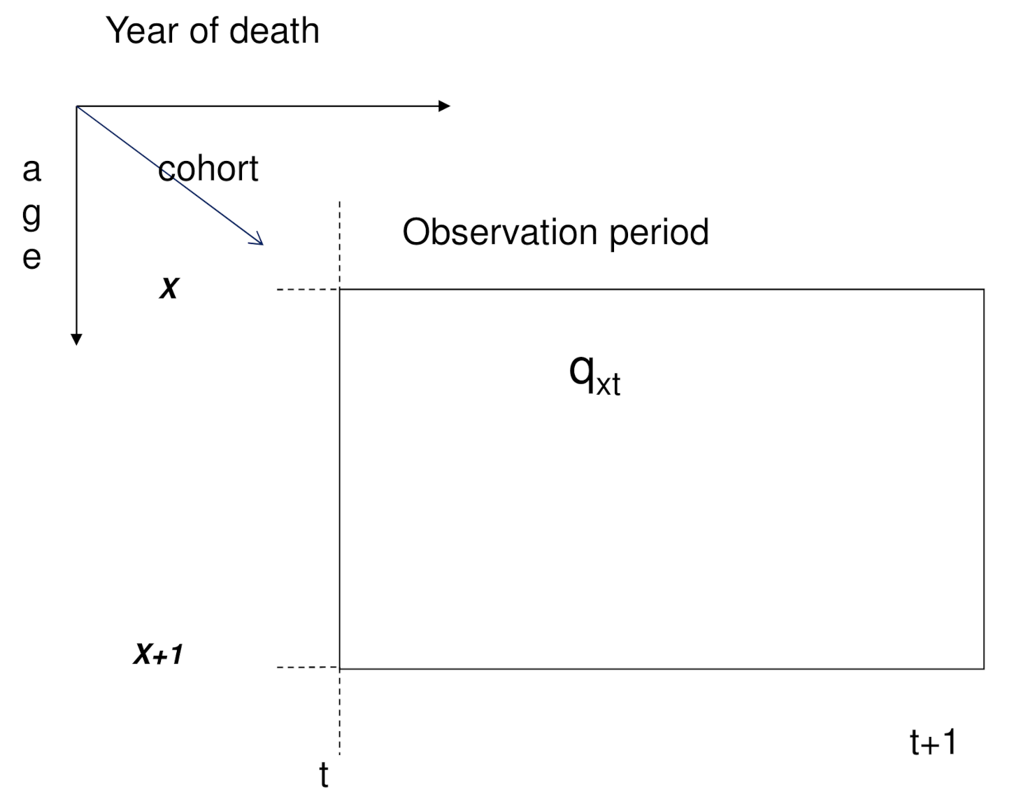
2.1. Lee-Carter Models
2.2. Mortality Indicators
2.3. Block-Bootstrap Prediction Intervals
2.4. ANOVA for Functional Data Analysis
3. Results
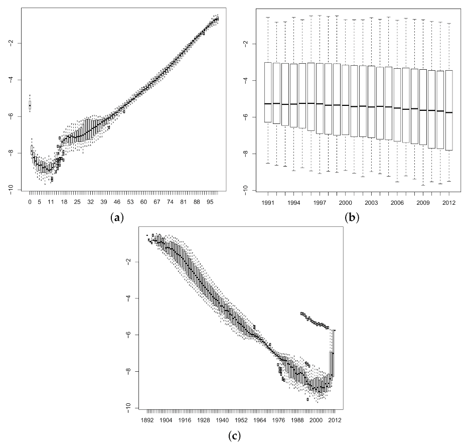
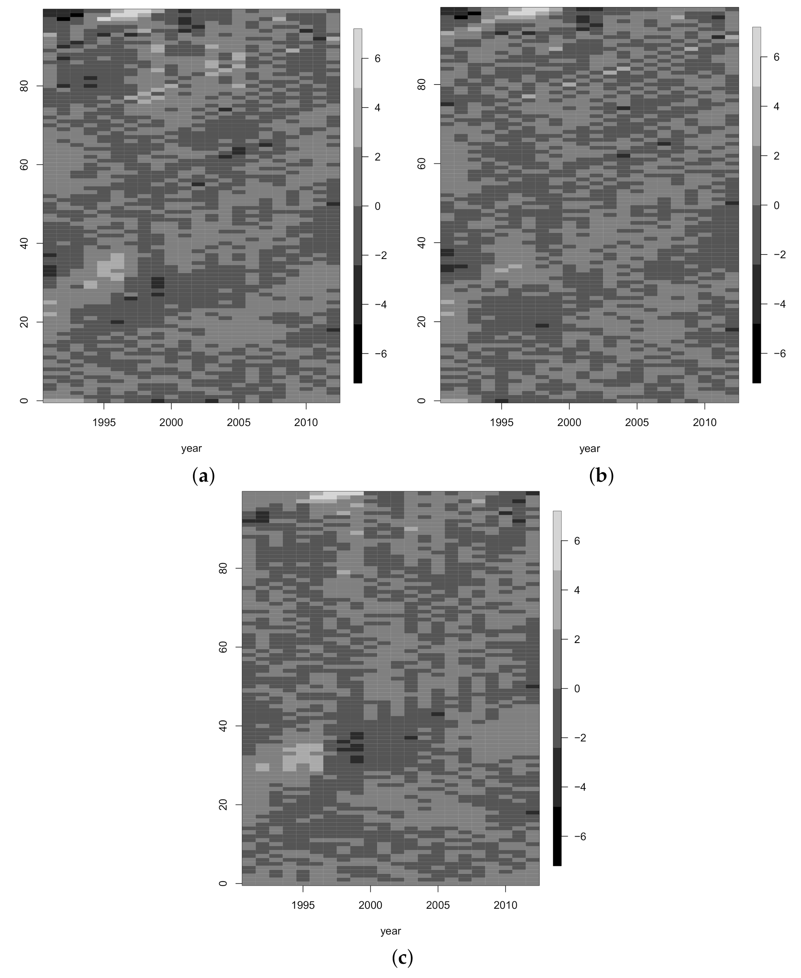
3.1. Model Fitting
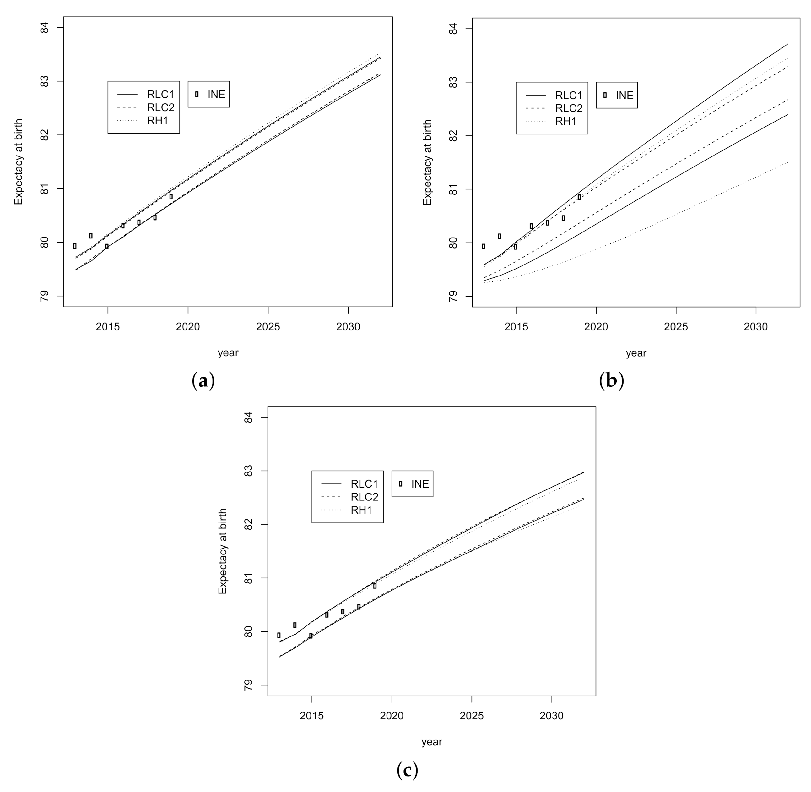
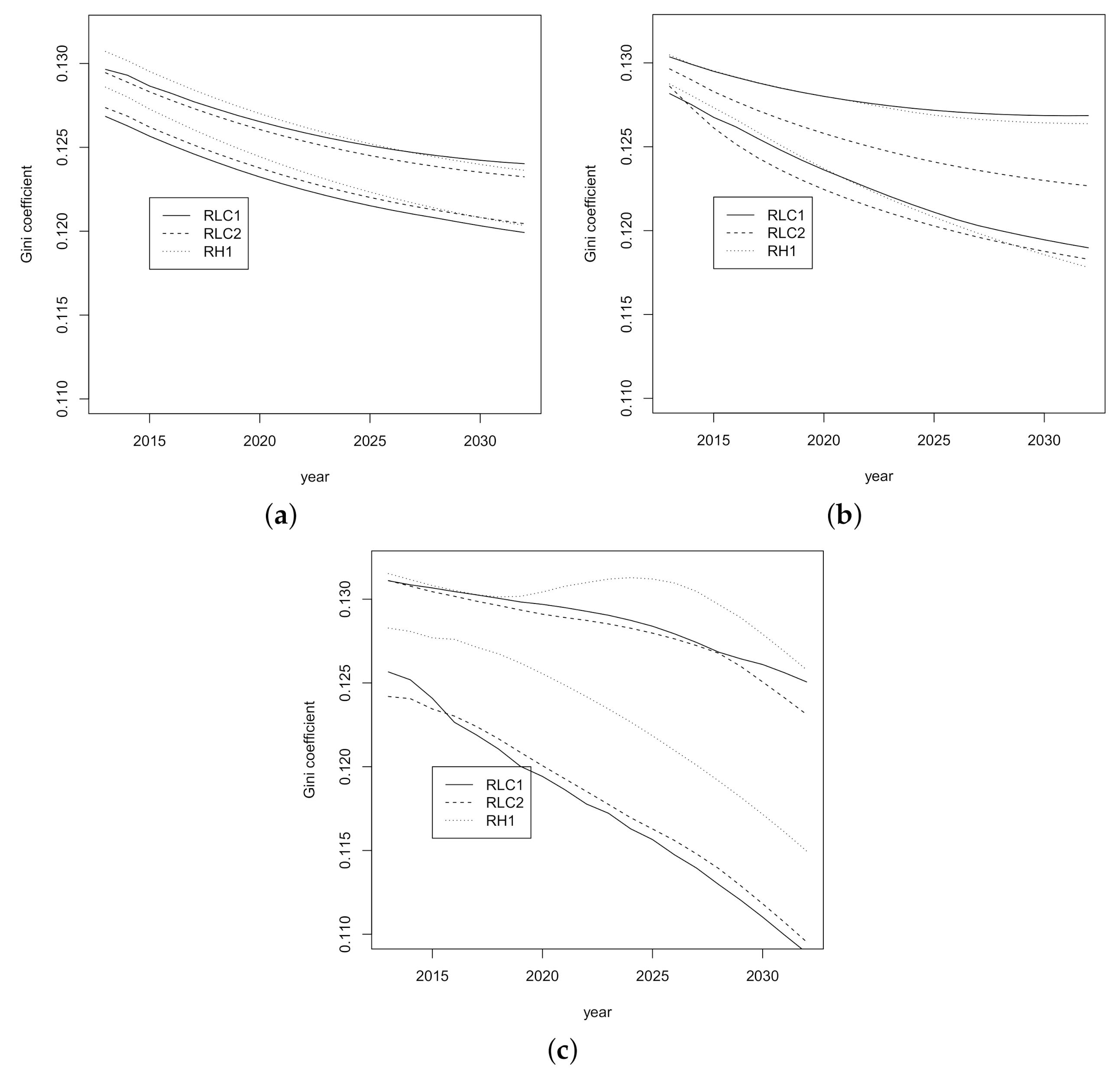
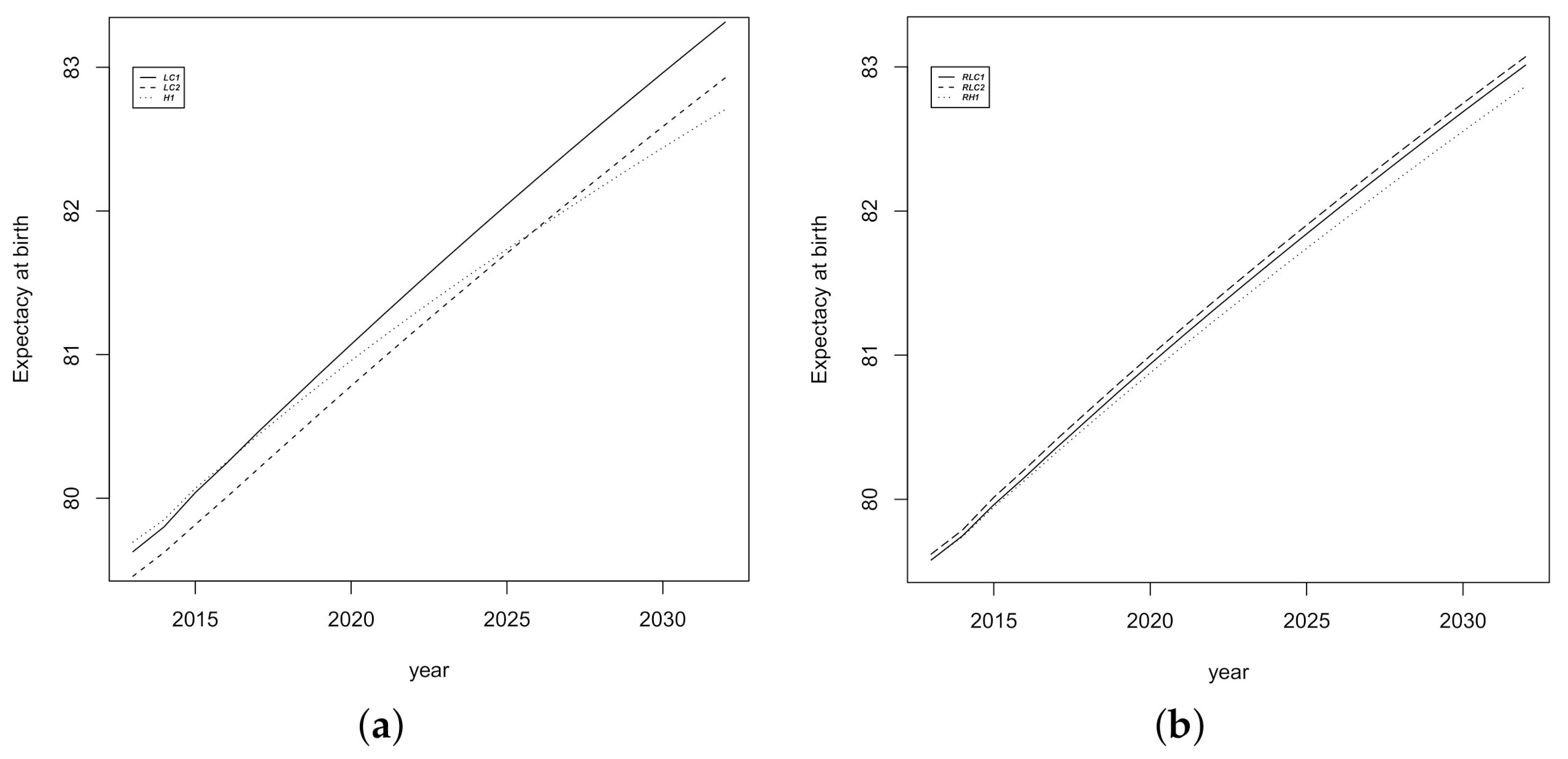
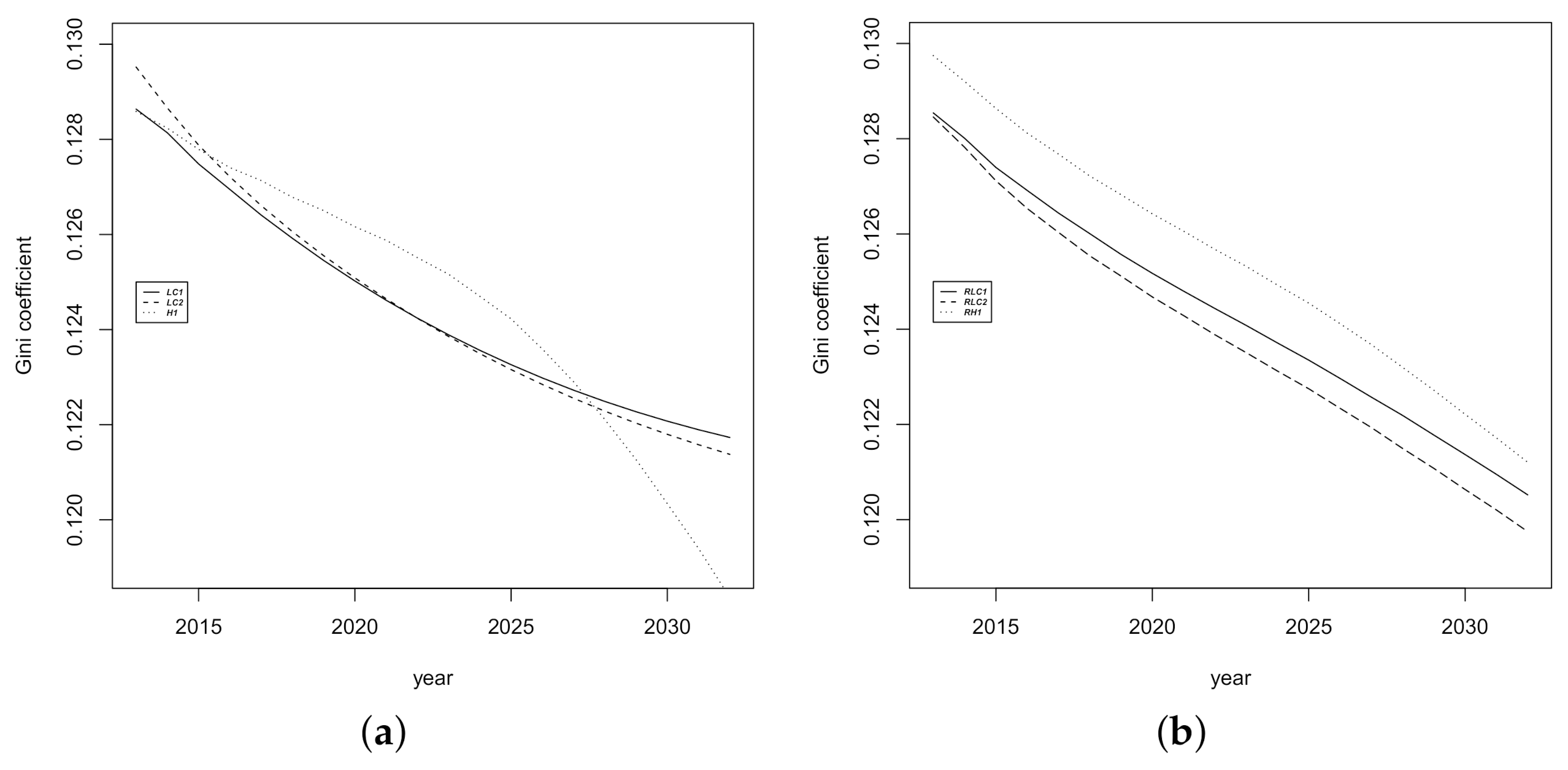
3.2. Prediction Intervals for Mortality Indicators
3.3. ANOVA for Functional Data Analysis
4. Conclusions
Author Contributions
Funding
Institutional Review Board Statement
Informed Consent Statement
Data Availability Statement
Acknowledgments
Conflicts of Interest
References
- Vaupel, J.W. Biodemography of human ageing. Nature 2010, 464, 536–542. [Google Scholar] [CrossRef] [Green Version]
- Atance, D.; Balbás, A.; Navarro, E. Constructing dynamic life tables with a single-factor model. Decis. Econ. Financ. 2020, 43, 787–825. [Google Scholar] [CrossRef]
- Lee, R.; Carter, L. Modelling and forecasting U.S. mortality. J. Am. Stat. Assoc. 1992, 87, 659–671. [Google Scholar]
- Azman, S.; Pathmanathan, D. The GLM framework of the Lee-Carter model: A multi-country study. J. Appl. Stat. 2020, 1–12. [Google Scholar] [CrossRef]
- Villegas, A.M.; Kaishev, V.K.; Millossovich, P. StMoMo: An R Package for Stochastic Mortality Modeling. J. Stat. Softw. 2018, 84, 1–38. [Google Scholar] [CrossRef] [Green Version]
- Debón, A.; Martínez-Ruiz, F.; Montes, F. Temporal Evolution of Mortality Indicators. N. Am. Actuar. J. 2012, 16, 364–377. [Google Scholar] [CrossRef]
- Debón, A.; Chaves, L.; Haberman, S.; Villa, F. Characterization of between-group inequality of longevity in European Union countries. Insur. Math. Econ. 2017, 75, 151–165. [Google Scholar] [CrossRef] [Green Version]
- Liu, X.; Braun, W.J. Investigating Mortality Uncertainty Using the Block Bootstrap. J. Probab. Stat. 2010, 2010, 385–399. [Google Scholar] [CrossRef] [Green Version]
- Lazar, D.; Denuit, M.M. A multivariate time series approach to projected life tables. Appl. Stoch. Model. Bus. Ind. 2009, 25, 806–823. [Google Scholar] [CrossRef]
- Debón, A.; Martínez-Ruiz, F.; Montes, F. A geostatistical approach for dynamic life tables: The effect of mortality on remaining lifetime and annuities. Insur. Math. Econ. 2010, 47, 327–336. [Google Scholar] [CrossRef] [Green Version]
- Hyndman, R.J.; Booth, H. Stochastic population forecasts using functional data models for mortality, fertility and migration. Int. J. Forecast. 2008, 24, 323–342. [Google Scholar] [CrossRef]
- Greenshtein, E. Best subset selection, persistence in high-dimensional statistical learning and optimization under l1 constraint. Ann. Stat. 2006, 34, 2367–2386. [Google Scholar] [CrossRef] [Green Version]
- Booth, H.; Hyndman, R.J.; Tickle, L.; de Jong, P. Lee-Carter mortality forecasting: A multi-country comparison of variants and extensions. Demogr. Res. 2006, 15, 289–310. [Google Scholar] [CrossRef]
- Cairns, A.J.; Blake, D.; Dowd, K.; Coughlan, G.D.; Epstein, D.; Khalaf-Allah, M. Mortality density forecasts: An analysis of six stochastic mortality models. Insur. Math. Econ. 2011, 48, 355–367. [Google Scholar] [CrossRef] [Green Version]
- Shang, H.L.; Booth, H.; Hyndman, R. Point and interval forecasts of mortality rates and life expectancy: A comparison of ten principal component methods. Demogr. Res. 2011, 25, 173–214. [Google Scholar] [CrossRef] [Green Version]
- Pitacco, E.; Denuit, M.; Haberman, S.; Olivieri, A. Modelling Longevity Dynamics for Pensions and Annuity Business; Oxford University Press: Oxford, UK, 2009. [Google Scholar]
- Brouhns, N.; Denuit, M.; Vermunt, J. Measuring the longevity risk in mortality projections. Bull. Swiss Assoc. Actuar. 2002, 2, 105–130. [Google Scholar]
- Currie, I.D. On fitting generalized linear and non-linear models of mortality. Scand. Actuar. J. 2016, 2016, 356–383. [Google Scholar] [CrossRef]
- Booth, H.; Maindonald, J.; Smith, L. Applying Lee-Carter under conditions of variable mortality decline. Popul. Stud. 2002, 56, 325–336. [Google Scholar] [CrossRef] [PubMed]
- Renshaw, A.; Haberman, S. Lee-Carter mortality forecasting with age specific enhancement. Insur. Math. Econ. 2003, 33, 255–272. [Google Scholar] [CrossRef]
- Turner, H.; Firth, D. Generalized Nonlinear Models in R: An Overview of the Gnm Package, R package version 1.1-1; R Foundation for Statistical Computing: Vienna, Austria, 2020. [Google Scholar]
- R Core Team. R: A Language and Environment for Statistical Computing; R Foundation for Statistical Computing: Vienna, Austria, 2020. [Google Scholar]
- Debón, A.; Montes, F.; Puig, F. Modelling and Forecasting mortality in Spain. Eur. J. Oper. Res. 2008, 189, 624–637. [Google Scholar] [CrossRef] [Green Version]
- Haberman, S.; Renshaw, A. A comparative study of parametric mortality projection models. Insur. Math. Econ. 2011, 48, 35–55. [Google Scholar] [CrossRef] [Green Version]
- Renshaw, A.; Haberman, S. A cohort-based extension to the Lee-Carter model for mortality reduction factors. Insur. Math. Econ. 2006, 38, 556–570. [Google Scholar] [CrossRef]
- Hyndman, R.J.; Shahid Ullah, M. Robust forecasting of mortality and fertility rates: A functional data approach. Comput. Stat. Data Anal. 2007, 51, 4942–4956. [Google Scholar] [CrossRef] [Green Version]
- Cairns, A.J.; Blake, D.; Dowd, K.; Coughlan, G.D.; Epstein, D.; Ong, A.; Balevich, I. A quantitative comparison of stochastic mortality models using data from England and Wales and the United States. N. Am. Actuar. J. 2009, 13, 1–35. [Google Scholar] [CrossRef]
- Hunt, A.; Villegas, A.M. Robustness and convergence in the Lee–Carter model with cohort effects. Insur. Math. Econ. 2015, 64, 186–202. [Google Scholar] [CrossRef]
- Haberman, S.; Renshaw, A. On age-period-cohort parametric mortality rate projections. Insur. Math. Econ. 2009, 45, 255–270. [Google Scholar] [CrossRef] [Green Version]
- Canudas-Romo, V. Three measures of longevity: Time trends and record values. Demogr. 2010, 47, 299–312. [Google Scholar] [CrossRef]
- Canudas-Romo, V. The modal age at death and the shifting mortality hypothesis. Demogr. Res. 2008, 19, 1179–1204. [Google Scholar] [CrossRef]
- Shkolnikov, V.; Andreev, E.; Begun, A. Gini coefficient as a life table function: Computation from discrete data, decomposition of differences and empirical examples. Demogr. Res. 2003, 8, 305–358. [Google Scholar] [CrossRef] [Green Version]
- Brouhns, N.; Denuit, M.; Keilegom, I.V. Bootstrapping Poisson log-bilinear model for mortality forecasting. Scand. Actuar. J. 2005, 2005, 212–224. [Google Scholar] [CrossRef]
- Koissi, M.; Shapiro, A.; Högnäs, G. Evaluating and extending the Lee-Carter model for mortality forecasting confidence interval. Insur. Math. Econ. 2006, 38, 1–20. [Google Scholar] [CrossRef]
- Efron, B.; Tibshirani, R. An Introduction to the Bootstrap; Chapman & Hall: New York, NY, USA; London, UK, 1993. [Google Scholar]
- Cuevas, A.; Febrero-Bande, M.; Fraiman, R. An anova test for functional data. Comput. Stat. Data Anal. 2004, 47, 111–122. [Google Scholar] [CrossRef]
- Martínez-Camblor, P.; Corral, N. Repeated measures analysis for functional data. Comput. Stat. Data Anal. 2011, 55, 3244–3256. [Google Scholar] [CrossRef]
- Abramovich, F.; Angelini, C. Testing in mixed-effects FANOVA models. J. Stat. Plan. Inference 2006, 136, 4326–4348. [Google Scholar] [CrossRef]
- Antoniadis, A.; Sapatinas, T. Estimation and inference in functional mixed-effects models. Comput. Stat. Data Anal. 2007, 51, 4793–4813. [Google Scholar] [CrossRef]
- Cuesta-Albertos, J.; Febrero-Bande, M. A simple multiway ANOVA for functional data. TEST 2010, 19, 537–557. [Google Scholar] [CrossRef]
- Muriel, S.; Cantalapiedra, M.; López, F. Towards Advanced Methods for Computing Life Tables; Technical Report. Instituto Nacional de Estadística, 2010. Available online: https://www.ine.es/ss/Satellite?L=es_ES&c=INEDocTrabajo_C&cid=1259925434773&p=1254735839320&pagename=MetodologiaYEstandares%2FINELayout (accessed on 10 May 2011).
- Elandt-Johnson, R.; Johnson, N. Survival Models and Data Analysis; Wiley: New York, NY, USA, 1980. [Google Scholar]
- Febrero-Bande, M.; Oviedo de la Fuente, M. Statistical Computing in Functional Data Analysis: The R Package fda.usc. J. Stat. Softw. 2012, 51, 1–28. [Google Scholar] [CrossRef] [Green Version]
- Benjamini, Y.; Yekutieli, D. The control of the false discovery rate in multiple testing under dependency. Ann. Stat. 2001, 29, 1165–1188. [Google Scholar]
- Shang, H.; Haberman, S. Forecasting age distribution of death counts: An application to annuity pricing. Ann. Actuar. Sci. 2020, 14, 150–169. [Google Scholar] [CrossRef] [Green Version]
- Bozikas, A.; Pitselis, G. An empirical study on stochastic mortality modelling under the age-period-cohort framework: The case of greece with applications to insurance pricing. Risks 2018, 6, 44. [Google Scholar] [CrossRef] [Green Version]
- International Monetary Fund. The Financial Impact of Longevity Risk. Technical Report. 2012. Available online: https://www.imf.org/~/media/Websites/IMF/imported-flagship-issues/external/pubs/ft/GFSR/2012/01/pdf/_c4pdf.ashx (accessed on 8 May 2012).


| Model | ||||
|---|---|---|---|---|
| LC1 | LC2 | H1 | ||
| LC1 | N | N | N | |
| Sample | RLC2 | N | N | N |
| RH1 | N | N | N | |
| LC1 | LC2 | H1 | |
|---|---|---|---|
| Deviance | 2911.45 | 2136.05 | 2192.48 |
| Number of parameters | 100 + 22 + 100 | 100 + 22 + 100 + 121 |
| Life Expectancy at Birth | Life Expectancy at 65 | |||||||||||||
|---|---|---|---|---|---|---|---|---|---|---|---|---|---|---|
| RLC1 | RLC2 | RH1 | RLC1 | RLC2 | RH1 | |||||||||
| Year | INE | p | p | p | p | p | p | INE | p | p | p | p | p | p |
| 2013 | 79.93 | 79.46 | 79.73 | 79.49 | 79.68 | 79.49 | 79.71 | 18.92 | 18.59 | 18.76 | 18.62 | 18.72 | 18.62 | 18.74 |
| 2014 | 80.12 | 79.64 | 79.90 | 79.70 | 79.84 | 79.65 | 79.89 | 19.06 | 18.71 | 18.86 | 18.73 | 18.82 | 18.72 | 18.86 |
| 2015 | 79.92 | 79.87 | 80.14 | 79.92 | 80.08 | 79.90 | 80.12 | 18.79 | 18.84 | 19.01 | 18.87 | 18.97 | 18.87 | 19.00 |
| 2016 | 80.31 | 80.06 | 80.35 | 80.13 | 80.29 | 80.10 | 80.33 | 19.14 | 18.97 | 19.14 | 19.00 | 19.10 | 18.99 | 19.14 |
| 2017 | 80.37 | 80.27 | 80.57 | 80.34 | 80.50 | 80.31 | 80.55 | 19.12 | 19.10 | 19.27 | 19.13 | 19.24 | 19.12 | 19.27 |
| 2018 | 80.46 | 80.47 | 80.77 | 80.54 | 80.71 | 80.51 | 80.76 | 19.22 | 19.23 | 19.41 | 19.26 | 19.37 | 19.25 | 19.41 |
| 2019 | 80.85 | 80.66 | 80.98 | 80.74 | 80.92 | 80.72 | 80.97 | 19.52 | 19.35 | 19.55 | 19.39 | 19.50 | 19.38 | 19.54 |
| 2020 | 80.86 | 81.19 | 80.94 | 81.12 | 80.92 | 81.18 | 19.48 | 19.68 | 19.52 | 19.63 | 19.51 | 19.67 | ||
| 2021 | 81.05 | 81.39 | 81.14 | 81.32 | 81.12 | 81.38 | 19.61 | 19.82 | 19.64 | 19.77 | 19.64 | 19.81 | ||
| 2022 | 81.24 | 81.59 | 81.33 | 81.52 | 81.31 | 81.58 | 19.73 | 19.95 | 19.77 | 19.90 | 19.76 | 19.94 | ||
| 2023 | 81.43 | 81.78 | 81.53 | 81.72 | 81.50 | 81.77 | 19.86 | 20.09 | 19.90 | 20.03 | 19.89 | 20.07 | ||
| 2024 | 81.62 | 81.98 | 81.72 | 81.91 | 81.69 | 81.97 | 19.98 | 20.22 | 20.02 | 20.16 | 20.02 | 20.20 | ||
| 2025 | 81.80 | 82.17 | 81.91 | 82.10 | 81.88 | 82.16 | 20.11 | 20.35 | 20.15 | 20.29 | 20.14 | 20.33 | ||
| 2026 | 81.99 | 82.37 | 82.10 | 82.29 | 82.07 | 82.36 | 20.23 | 20.49 | 20.27 | 20.42 | 20.27 | 20.46 | ||
| 2027 | 82.17 | 82.56 | 82.28 | 82.47 | 82.25 | 82.54 | 20.35 | 20.62 | 20.40 | 20.55 | 20.39 | 20.59 | ||
| 2028 | 82.35 | 82.75 | 82.46 | 82.66 | 82.43 | 82.73 | 20.48 | 20.75 | 20.52 | 20.67 | 20.51 | 20.72 | ||
| 2029 | 82.52 | 82.93 | 82.64 | 82.84 | 82.61 | 82.92 | 20.60 | 20.88 | 20.64 | 20.80 | 20.64 | 20.85 | ||
| 2030 | 82.70 | 83.11 | 82.81 | 83.02 | 82.79 | 83.10 | 20.72 | 21.00 | 20.77 | 20.93 | 20.76 | 20.98 | ||
| 2031 | 82.87 | 83.29 | 82.99 | 83.20 | 82.96 | 83.28 | 20.84 | 21.13 | 20.89 | 21.05 | 20.88 | 21.11 | ||
| 2032 | 83.04 | 83.47 | 83.16 | 83.37 | 83.14 | 83.46 | 20.96 | 21.26 | 21.01 | 21.18 | 21.00 | 21.23 | ||
| Model | Residual | Model × Residual | |
|---|---|---|---|
| Indicator | |||
| R | R | R | |
| R | R | R | |
| Gini index | R | R | R |
| Modal age | R | R | R |
| Model | |||
| R | R | R | |
| R | R | R | |
| Gini index | R | R | R |
| Modal age | R | R | R |
| Sample | |||
| R | R | R | |
| R | R | R | |
| Gini index | R | R | R |
| Modal age | R | R | R |
Publisher’s Note: MDPI stays neutral with regard to jurisdictional claims in published maps and institutional affiliations. |
© 2021 by the authors. Licensee MDPI, Basel, Switzerland. This article is an open access article distributed under the terms and conditions of the Creative Commons Attribution (CC BY) license (http://creativecommons.org/licenses/by/4.0/).
Share and Cite
Debón, A.; Haberman, S.; Montes, F.; Otranto, E. Do Different Models Induce Changes in Mortality Indicators? That Is a Key Question for Extending the Lee-Carter Model. Int. J. Environ. Res. Public Health 2021, 18, 2204. https://0-doi-org.brum.beds.ac.uk/10.3390/ijerph18042204
Debón A, Haberman S, Montes F, Otranto E. Do Different Models Induce Changes in Mortality Indicators? That Is a Key Question for Extending the Lee-Carter Model. International Journal of Environmental Research and Public Health. 2021; 18(4):2204. https://0-doi-org.brum.beds.ac.uk/10.3390/ijerph18042204
Chicago/Turabian StyleDebón, Ana, Steven Haberman, Francisco Montes, and Edoardo Otranto. 2021. "Do Different Models Induce Changes in Mortality Indicators? That Is a Key Question for Extending the Lee-Carter Model" International Journal of Environmental Research and Public Health 18, no. 4: 2204. https://0-doi-org.brum.beds.ac.uk/10.3390/ijerph18042204