
Indoor Air Quality in Domestic Environments during Periods Close to Italian COVID-19 Lockdown


Abstract
:1. Introduction
2. Materials and Methods
2.1. Study Area Description
2.2. Apartment Characteristics
2.3. IAQ Monitoring
2.4. Meteorological and Atmoshere Conditions Characteristics
3. Results
3.1. Outdoor Parameters
3.2. Indoor AIQ Parameters
3.2.1. Indoor Temperature
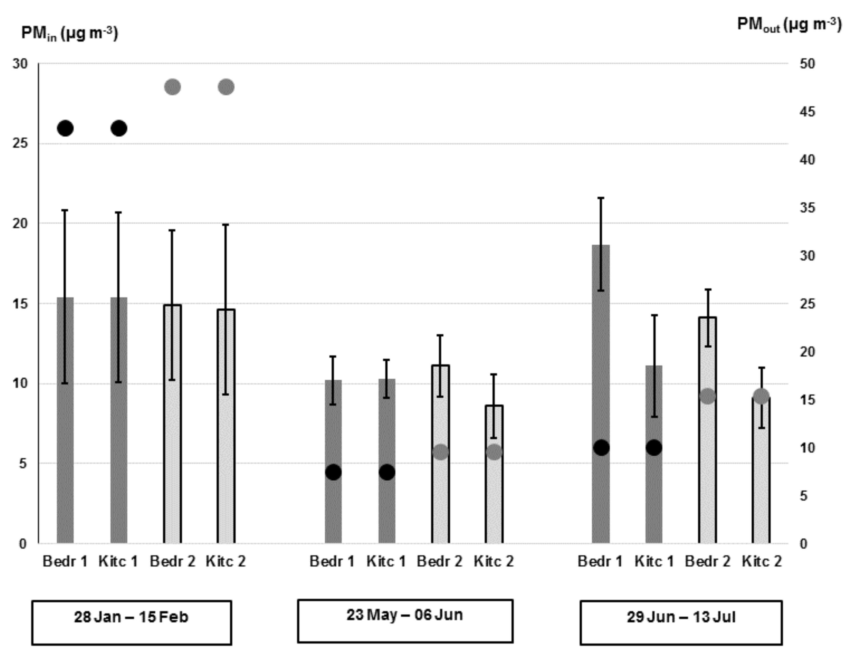
3.2.2. Indoor PM2.5
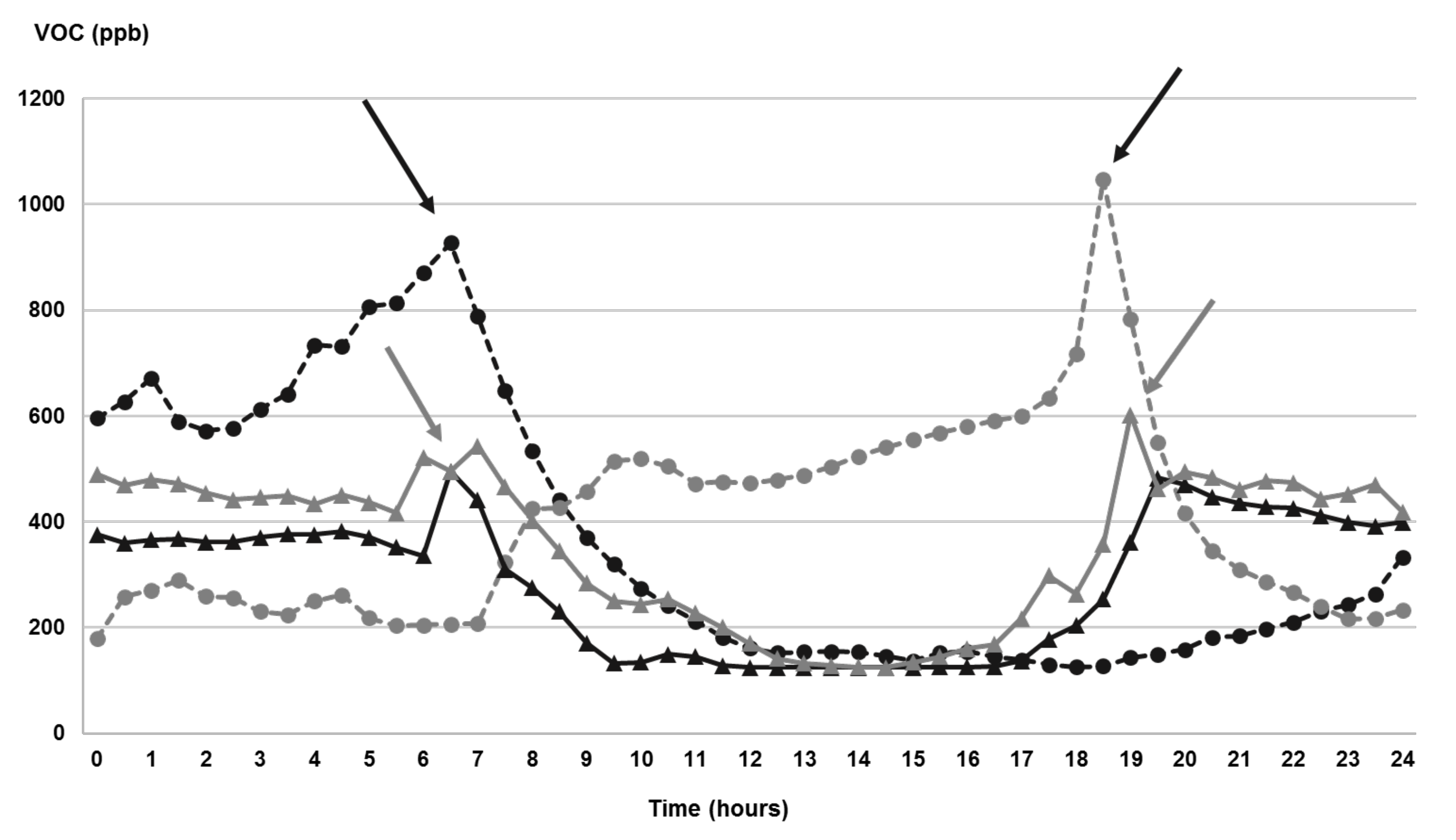
3.2.3. VOCs and CO2
4. Conclusions
Supplementary Materials
Author Contributions
Funding
Institutional Review Board Statement
Informed Consent Statement
Data Availability Statement
Conflicts of Interest
References
- Health Effects Institute. State of Global Air 2020; Special Report; Health Effects Institute: Boston, MA, USA, 2020. [Google Scholar]
- Shaddick, G.; Salter, J.M.; Peuch, V.-H.; Ruggeri, G.; Thomas, M.L.; Mudu, P.; Tarasova, O.; Baklanov, A.; Gumy, S. Global Air Quality: An Inter-Disciplinary Approach to Exposure Assessment for Burden of Disease Analyses. Atmosphere 2021, 12, 48. [Google Scholar] [CrossRef]
- Settimo, G.; Manigrasso, M.; Avino, P. Indoor air quality: A focus on the European legislation and state-of-the-art research in Italy. Atmosphere 2020, 11, 370. [Google Scholar] [CrossRef] [Green Version]
- Leung, D.Y.C. Outdoor-indoor air pollution in urban environment: Challenges and opportunity. Front. Environ. Sci. 2015, 2, 1–7. [Google Scholar] [CrossRef]
- Li, Z.; Wen, Q.; Zhang, R. Sources, health effects and control strategies of indoor fine particulate matter (PM2.5): A review. Sci. Total Environ. 2017, 586, 610–622. [Google Scholar] [CrossRef]
- Zar, H.J.; Ferkol, T.W. The global burden of respiratory disease—Impact on child health. Pediatr. Pulmonol. 2014, 49, 430–434. [Google Scholar] [CrossRef]
- Bari, M.A.; Kindzierski, W.B.; Wheeler, A.; Héroux, M.È.; Wallace, L.A. Source apportionment of indoor and outdoor volatile organic compounds at homes in Edmonton, Canada. Build. Environ. 2015, 90, 114–124. [Google Scholar] [CrossRef]
- Goel, S.G.; Somwanshi, S.; Mankar, S.; Srimuruganandam, B.; Gupta, R. Characteristics of indoor air pollutants and estimation of their exposure dose. Air Qual. Atmos. Health 2021. [Google Scholar] [CrossRef]
- Yassin, M.F.; Al Thaqeb, B.E.Y.; Al-Mutiri, E.A.E. Assessment of indoor PM2.5 in different residential environments. Atmos. Environ. 2012, 56, 65–68. [Google Scholar] [CrossRef]
- Martins, N.R.; Carrilho da Graça, G. Impact of PM2.5 in indoor urban environments: A review. Sustain. Cities Soc. 2018, 42, 259–275. [Google Scholar] [CrossRef]
- Tofful, L.; Perrino, C. Chemical composition of indoor and outdoor PM2.5 in three schools in the city of Rome. Atmosphere 2015, 6, 1422–1443. [Google Scholar] [CrossRef] [Green Version]
- Nadali, A.; Arfaeinia, H.; Asadgol, Z.; Fahiminia, M. Indoor and outdoor concentration of PM10, PM2.5 and PM1 in residential building and evaluation of negative air ions (NAIs) in indoor PM removal. Environ. Pollut. Bioavailab. 2020, 32, 47–55. [Google Scholar] [CrossRef] [Green Version]
- McGill, G.; Oyedele, L.O.; McAllister, K. Case study investigation of indoor air quality in mechanically ventilated and naturally ventilated UK social housing. Int. J. Sustain. Built. Environ. 2015, 4, 58–77. [Google Scholar] [CrossRef] [Green Version]
- Vardoulakis, S.; Giagloglou, E.; Steinle, S.; Davis, A.; Sleeuwenhoek, A.; Galea, K.S.; Dixon, K.; Crawford, J.O. Indoor exposure to selected air pollutants in the home environment: A systematic review. Int. J. Environ. Res. Public Health 2020, 17, 8972. [Google Scholar] [CrossRef] [PubMed]
- Sánka, I.; Földváry, V. Indoor Air Quality of Residential Building Before and After Renovation. Slovak J. Civ. Eng. 2017, 25, 1–6. [Google Scholar] [CrossRef] [Green Version]
- Földváry, V.; Bekö, G.; Langer, S.; Arrhenius, K.; Petráš, D. Effect of energy renovation on indoor air quality in multifamily residential buildings in Slovakia. Build. Environ. 2017, 122, 363–372. [Google Scholar] [CrossRef] [Green Version]
- Broderick, Á.; Byrne, M.; Armstrong, S.; Sheahan, J.; Coggins, A.M. A pre and post evaluation of indoor air quality, ventilation, and thermal comfort in retrofitted co-operative social housing. Build. Environ. 2017, 122, 126–133. [Google Scholar] [CrossRef]
- Schweizer, C.; Edwards, R.D.; Bayer-Oglesby, L.; Gauderman, W.J.; Ilacqua, V.; Jantunen, M.J.; Lai, H.K.; Nieuwenhuijsen, M.; Künzli, N. Indoor time-microenvironment-activity patterns in seven regions of Europe. J. Expo. Sci. Environ. Epidemiol. 2007, 17, 170–181. [Google Scholar] [CrossRef] [Green Version]
- Fernández-Agüera, J.; Domínguez-Amarillo, S.; Alonso, C.; Martín-Consuegra, F. Thermal comfort and indoor air quality in low-income housing in Spain: The influence of airtightness and occupant behavior. Energy Build. 2019, 199, 102–114. [Google Scholar] [CrossRef]
- Langer, S.; Bekö, G.; Bloom, E.; Widheden, A.; Ekberg, L. Indoor air quality in passive and conventional new houses in Sweden. Build. Environ. 2015, 93, 92–100. [Google Scholar] [CrossRef]
- Fernández-Agüera, J.; Dominguez-Amarillo, S.; Fornaciari, M.; Orlandi, F. TVOCs and PM2.5 in naturally ventilated homes: Three case studies in a mild climate. Sustainability 2019, 11, 6225. [Google Scholar] [CrossRef] [Green Version]
- Moreno-Rangel, A.; Sharpe, T.; Musau, F.; McGill, G. Field evaluation of a low-cost indoor air quality monitor to quantify exposure to pollutants in residential environments. J. Sens. Sens. Syst. 2018, 7, 373–388. [Google Scholar] [CrossRef] [Green Version]
- Sousan, S.; Koehler, K.; Hallett, L.; Peters, T.M. Evaluation of consumer monitors to measure particulate matter. J. Aerosol. Sci. 2017, 107, 123–133. [Google Scholar] [CrossRef] [Green Version]
- Liu, X.; Jayaratne, R.; Thai, P.; Kuhn, T.; Zing, I.; Christensen, B.; Lamont, R.; Dunbabin, M. Low-cost sensors as an alternative for long-term air quality monitoring. Environ. Res. 2020, 185, 109438. [Google Scholar] [CrossRef] [PubMed]
- Chojer, H.; Branco, P.T.B.; Martins, F.; Alvim-Ferraz, M.C.M.; Sousa, S.I.V. Development of low-cost indoor air quality monitoring devices: Recent advancements. Sci. Total Environ. 2020, 727, 138385. [Google Scholar] [CrossRef]
- Manibusan, S.; Mainelis, G. Performance of four consumer-grade air pollution measurement devices in different residences. Aerosol. Air Qual. Res. 2020, 20, 217–230. [Google Scholar] [CrossRef] [PubMed] [Green Version]
- Lowther, S.; Jones, K.C.; Wang, X.; Whyatt, J.D.; Wild, O.; Booker, D. Particulate Matter Measurement Indoors: A Review of Metrics, Sensors, Needs, and Applications. Environ. Sci. Technol. 2019, 53, 11644–11656. [Google Scholar] [CrossRef]
- Cameletti, M. The Effect of Corona Virus Lockdown on Air Pollution: Evidence from the City of Brescia in Lombardia Region (Italy). Atmos. Environ. 2020, 239, 117794. [Google Scholar] [CrossRef]
- Saini, J.; Dutta, M.; Marques, G. Indoor Air Quality Monitoring Systems and COVID-19. Emerg. Technol. Era COVID-19 Pandemic 2021, 348, 133–147. [Google Scholar]
- PREPAIR-Po Regions Engaged to Policies of AIR. Available online: https://www.lifeprepair.eu/ (accessed on 28 March 2021).
- Guyot, G.; Sherman, M.H.; Walker, I.S. Smart ventilation energy and indoor air quality performance in residential buildings: A review. Energy Build. 2018, 165, 416–430. [Google Scholar] [CrossRef] [Green Version]
- Indoor Air Quality Monitoring Systems and COVID-19” Is the Paper Title, iAQ-Core Indoor Air Quality Sensor Module. Available online: https://www.sciosense.com/wp-content/uploads/documents/iaQ-Core-Datasheet.pdf (accessed on 8 April 2021).
- EN:12341. 2014. Available online: https://www.gazzettaufficiale.it/atto/serie_generale/PubblicazioneGazzetta=2017-02-09 (accessed on 28 March 2021).
- European Environmental Agency. Air Quality in Europe—2018 Report No 12/2018. 2018. Available online: papers2://publication/uuid/1D25F41B-C673-4FDA-AB71-CC5A2AD97FDD (accessed on 8 April 2021).
- Decesari, S.; Allan, J.; Plass-Duelmer, C.; Williams, B.J.; Paglione, M.; Facchini, M.C.C.; O’Dowd, C.; Harrison, R.M.; Gietl, J.K.; Coe, H.; et al. Measurements of the aerosol chemical composition and mixing state in the Po Valley using multiple spectroscopic techniques. Atmos. Chem. Phys. 2014, 4, 12109–12132. [Google Scholar] [CrossRef] [Green Version]
- Bigi, A.; Ghermandi, G.; Harrison, R.M. Analysis of the air pollution climate at a background site in the Po valley. J. Environ. Monit. 2012, 14, 552–563. [Google Scholar] [CrossRef] [Green Version]
- Pietrogrande, M.C.; Bacco, D.; Ferrari, S.; Ricciardelli, I.; Scotto, F.; Trentini, A.; Visentin, M. Characteristics and major sources of carbonaceous aerosols in PM2.5 in Emilia Romagna Region (Northern Italy) from four-year observations. Sci. Total Environ. 2016, 553, 172–183. [Google Scholar] [CrossRef]
- Khan, M.B.; Masiol, M.; Formenton, G.; Di Gilio, A.; de Gennaro, G.; Agostinelli, C.; Pavoni, B. Carbonaceous PM2.5 and secondary organic aerosol across the Veneto region (NE Italy). Sci. Total Environ. 2016, 542, 172–181. [Google Scholar] [CrossRef]
- Zagatti, E.; Russo, M.; Pietrogrande, M.C. On-Site Monitoring Indoor Air Quality in Schools: A Real-World Investigation to Engage High School Science Students. J. Chem. Educ. 2020, 97, 4069–4072. [Google Scholar] [CrossRef]
- The American Society of Heating R and A-CE (ASHRAE). Thermal environmental conditions for human occupancy. ANSI/ASHRAE Stand-55 2017, 7, 6. [Google Scholar]
- Santamouris, M.; Argiroudis, K.; Georgiou, M.; Pavlou, K.; Assimakopoulos, M.; Sfakianaki, K. Indoor air quality in fifty residences in Athens. Int. J. Vent. 2007, 5, 367–380. [Google Scholar] [CrossRef] [Green Version]
- Derbez, M.; Berthineau, B.; Cochet, V.; Lethrosne, M.; Pignon, C.; Riberon, J.; Kirchner, S. Indoor air quality and comfort in seven newly built, energy-efficient houses in France. Build. Environ. 2014, 72, 173–187. [Google Scholar] [CrossRef]
- Perrino, C.; Tofful, L.; Canepari, S. Chemical characterization of indoor and outdoor fine particulate matter in an occupied apartment in Rome, Italy. Indoor Air 2016, 26, 558–570. [Google Scholar] [CrossRef]
- WHO Guidelines for Indoor Air Quality: Selected Pollutants. Available online: https://www.euro.who.int/__data/assets/pdf_file/0009/128169/e94535.pdf (accessed on 28 February 2021).
- Ruggieri, S.; Longo, V.; Perrino, C.; Canepari, S.; Drago, G.; L’Abbate, L.; Balzan, M.; Cuttitta, G.; Scaccianoce, G.; Minardi, R.; et al. Indoor air quality in schools of a highly polluted south Mediterranean area. Indoor Air 2019, 29, 276–290. [Google Scholar] [CrossRef]
- Romagnoli, P.; Balducci, C.; Perilli, M.; Vichi, F.; Imperiali, A.; Cecinato, A. Indoor air quality at life and work environments in Rome, Italy. Environ. Sci. Pollut. Res. 2016, 23, 3503–3516. [Google Scholar] [CrossRef]
- Taylor, J.; Shrubsole, C.; Davies, M.; Biddulph, P.; Das, P.; Hamilton, I.; Vardoulakis, S.; Mavrogianni, A.; Jones, B.; Oikonomou, E. The modifying effect of the building envelope on population exposure to PM2.5 from outdoor sources. Indoor Air 2014, 24, 639–651. [Google Scholar] [CrossRef] [PubMed] [Green Version]
- Sun, X.; He, J.; Yang, X. Human breath as a source of VOCs in the built environment, Part II: Concentration levels, emission rates and factor analysis. Build. Environ. 2017, 123, 437–445. [Google Scholar] [CrossRef]


| Feature | Flat 1 | Flat 2 |
|---|---|---|
| Location | Rural (Medolla) | Urban (Ferrara) |
| Year of construction | 2012 | 1970 |
| N° occupants | 5 | 3 |
| N° pets | 4 | - |
| Ventilation system | Mechanically controlled windows Forced air recirculating | Natural ventilation |
| Heating system | Underfloor heating | Radiators |
| Cooling system | Heat pump (whole house unit) | - |
| Air conditioning | Underfloor air conditioning | Split units in rooms |
| Cookers | Induction | Gas |
| Period | Tout (°C) | RH%out | Outdoor PM2.5 (µg m−3) | Room | Tin (°C) | RH%in | Indoor PM2.5 (µg m−3) | PM2.5 I/O Ratio | VOCs (ppb) | CO2 (ppm) |
|---|---|---|---|---|---|---|---|---|---|---|
| 28 January–15 February | 12.0 ± 2.5 | 81.6 ± 11.8 | 43.3 ± 16.4 | Bed 1 | 20.2 ± 0.4 | 48.6 ± 2.3 | 15.4 ± 5.4 | 0.35 ± 0.12 | 306 ± 47 | 1106 ± 170 |
| Kitc 1 | 19.9 ± 0.2 | 48.4 ± 2.3 | 15.4 ± 5.3 | 0.33 ± 0.08 | 302 ± 54 | 1094 ± 196 | ||||
| 11.7 ± 2.3 | 75.8 ± 15.8 | 47.6 ± 17.1 | Bed 2 | 21.2 ± 0.3 | 48.5 ± 2.3 | 14.9 ± 4.7 | 0.37 ± 0.10 | 260 ± 52 | 940 ± 190 | |
| Kitc 2 | 21.4 ± 0.2 | 48.6 ± 2.3 | 14.6 ± 5.3 | 0.34 ± 0.08 | 317 ± 91 | 1147 ± 331 | ||||
| 23 May–6 June | 25.7 ± 3.5 | 63.5 ± 11.3 | 7.4 ± 1.6 | Bed 1 | 22.8 ± 0.3 | 52.2 ± 4.1 | 10.2 ± 1.5 | 1.12 ± 0.38 | 373 ± 66 | 1349 ± 238 |
| Kitc 1 | 23.4 ± 0.4 | 52.0 ± 4.0 | 10.3 ± 1.2 # | 1.13 ± 0.33 | 584 ± 92 # | 2116 ± 517 # | ||||
| 24.1 ± 3.2 | 54.3 ± 12.5 | 9.6 ± 2.1 | Bed 2 | 25.5 ± 0.6 | 52.1 ± 4.0 | 11.1 ± 1.9 | 1.59 ± 0.52 | 444 ± 96 | 1610 ± 347 | |
| Kitc 2 | 25.0 ± 0.6 | 52.0 ± 3.9 | 8.6 ± 2.0 | 1.22 ± 0.43 | 343 ± 60 | 1240 ± 219 | ||||
| 29 June–13 July | 30.8 ± 2.8 | 63.4 ± 6.2 | 10.0 ± 2.4 | Kitc 1 | 29.7 ± 1.0 | 46.9 ± 3.4 | 18.7 ± 2.9 # | 1.21 ± 0.26 | 271 ± 55 # | 954 ± 228 # |
| Kitc 1 | 24.7 ± 0.3 | 47.0 ± 3.3 | 11.1 ± 2.2 # | 0.74 ± 0.23 | 491 ± 85 # | 1783 ± 383 # | ||||
| 30.0 ± 2.7 | 63.4 ± 6.2 | 15.4 ± 3.9 | Bed 2 | 27.5 ± 0.4 | 46.3 ± 2.9 | 14.1 ± 1.8 | 1.47 ± 0.39 | 131 ± 52 | 470 ± 19 | |
| Kitc 2 | 27.2 ± 0.5 | 46.4 ± 3.0 | 9.1 ± 1.9 | 0.94 ± 0.26 | 361 ± 79 | 1284 ± 411 |
| Period | Room | Daytime PM2.5 (µg m−3) | Night PM2.5 (µg m−3) | Daytime VOCs (ppb) | Night VOCs (ppb) |
|---|---|---|---|---|---|
| 28 January–15 February | Bed 1 | 17.1 ± 7.4 | 13.1 ± 5.4 | 437 ± 92 * | 156 ± 15 |
| Kitc 1 | 19.1 ± 8.0 * | 10.4 ± 5.3 | 372 ± 89 * | 231 ± 32 | |
| Bed 2 | 15.8 ± 6.3 | 13.1 ± 4.7 | 314 ± 83 * | 219 ± 39 | |
| Kitc 2 | 17.6 ± 6.5 * | 11.1 ± 4.7 | 355 ± 93 * | 287 ± 75 | |
| 23 May–6 June | Bed 1 | 10.6 ± 17 | 9.6 ± 1.8 | 561 ± 139 * | 294 ± 52 |
| Kitc 1 | 10.5 ± 1.6 | 10.0 ± 1.61 # | 841 ± 185 * | 479 ± 136 | |
| Bed 2 | 10.9 ± 2.7 | 11.2 ± 1.61 | 576 ± 140 * | 384 ± 101 | |
| Kitc 2 | 9.9 ± 3.1 * | 7.2 ± 1.8 | 394 ± 82 | 317 ± 60 | |
| 29 June–13 July | Bed 1 | 19.0 ± 5.1 | 18.3 ± 4.7 # | 278 ± 68 # | 249 ± 46 # |
| Kitc 1 | 11.6 ± 5.7 | 10.4 ± 1.3 # | 630 ± 178 *# | 348 ± 72 | |
| Bed2 | 14.4 ± 1.7 | 13.7 ± 1.8 | 128 ± 3 | 133 ± 8 | |
| Kitc 2 | 9.4 ± 3.5 | 8.9 ± 1.5 | 391 ± 113 | 317 ± 119 |
| Period | Room | Indoor vs. Outdoor Temperature | Indoor vs. Outdoor PM2.5 |
|---|---|---|---|
| 28 January–15 February | Bed 1 | −0.057 | 0.734 ** |
| Kitc 1 | −0.079 | 0.731 ** | |
| Bed 2 | 0.307 | 0.842 ** | |
| Kitc 2 | 0.244 | 0.789 ** | |
| 23 May–6 June | Bed 1 | −0.380 | 0.395 |
| Kitc 1 | 0.274 | −0.035 | |
| Bed 2 | 0.687 * | −0.293 | |
| Kitc 2 | 0.802 ** | −0.455 | |
| 29 June–13 July | Bed 1 | 0.491 | 0.408 |
| Kitc 1 | −0.063 | 0.299 | |
| Bed 2 | 0.478 | 0.667 * | |
| Kitc 2 | −0.271 | 0.656 * |
Publisher’s Note: MDPI stays neutral with regard to jurisdictional claims in published maps and institutional affiliations. |
© 2021 by the authors. Licensee MDPI, Basel, Switzerland. This article is an open access article distributed under the terms and conditions of the Creative Commons Attribution (CC BY) license (https://creativecommons.org/licenses/by/4.0/).
Share and Cite
Pietrogrande, M.C.; Casari, L.; Demaria, G.; Russo, M. Indoor Air Quality in Domestic Environments during Periods Close to Italian COVID-19 Lockdown. Int. J. Environ. Res. Public Health 2021, 18, 4060. https://0-doi-org.brum.beds.ac.uk/10.3390/ijerph18084060
Pietrogrande MC, Casari L, Demaria G, Russo M. Indoor Air Quality in Domestic Environments during Periods Close to Italian COVID-19 Lockdown. International Journal of Environmental Research and Public Health. 2021; 18(8):4060. https://0-doi-org.brum.beds.ac.uk/10.3390/ijerph18084060
Chicago/Turabian StylePietrogrande, Maria Chiara, Lucia Casari, Giorgia Demaria, and Mara Russo. 2021. "Indoor Air Quality in Domestic Environments during Periods Close to Italian COVID-19 Lockdown" International Journal of Environmental Research and Public Health 18, no. 8: 4060. https://0-doi-org.brum.beds.ac.uk/10.3390/ijerph18084060