
Assessment of On-Board and Laboratory Gas Measurement Systems for Future Heavy-Duty Emissions Regulations

 , ,
, ,
Abstract
:1. Introduction
2. Materials and Methods
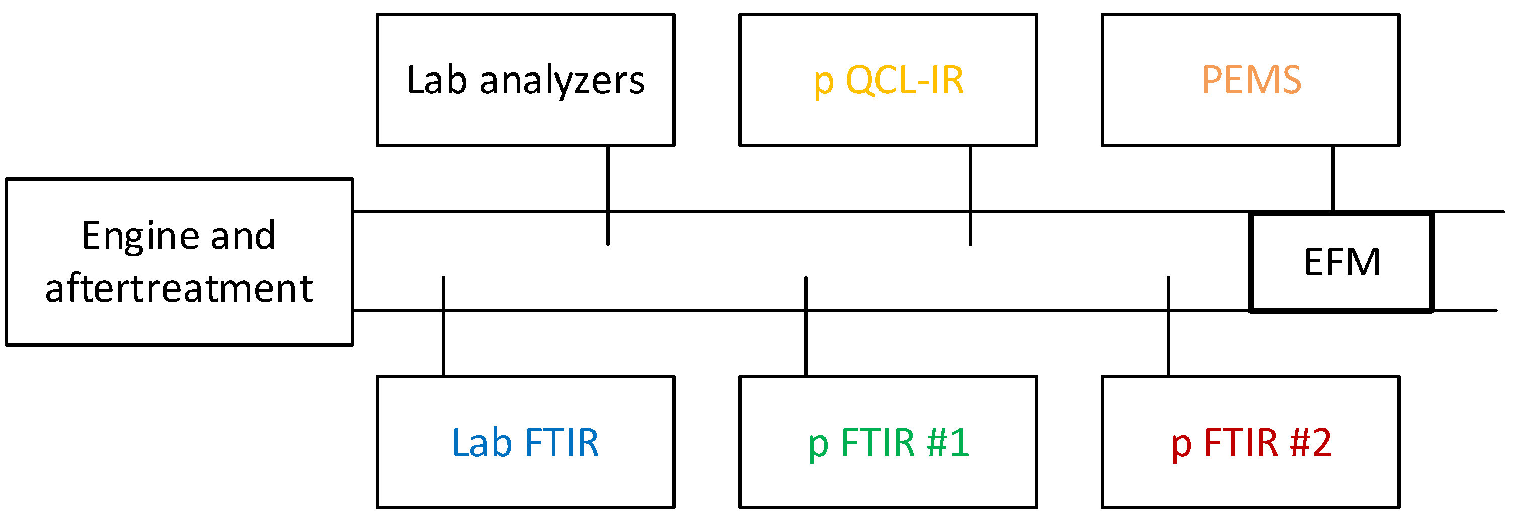
2.1. Setup
2.2. Instrumentation
- Linearity requirements: slope 0.99–1.01, R2 ≥ 0.998, SEE (standard error of estimate) ≤ 1% max, offset ≤ 0.5% max;
- Accuracy: ±2% of reading or ±0.3% of full scale (whichever is larger). For NH3 this requirement is ±3% of reading or 2 ppm whichever is larger);
- Limit of detection: no requirements, except for NH3 (<2 ppm). Typically, it is around 1–2 ppm for most gases.
2.3. Test Protocol
2.4. Calculations
3. Results
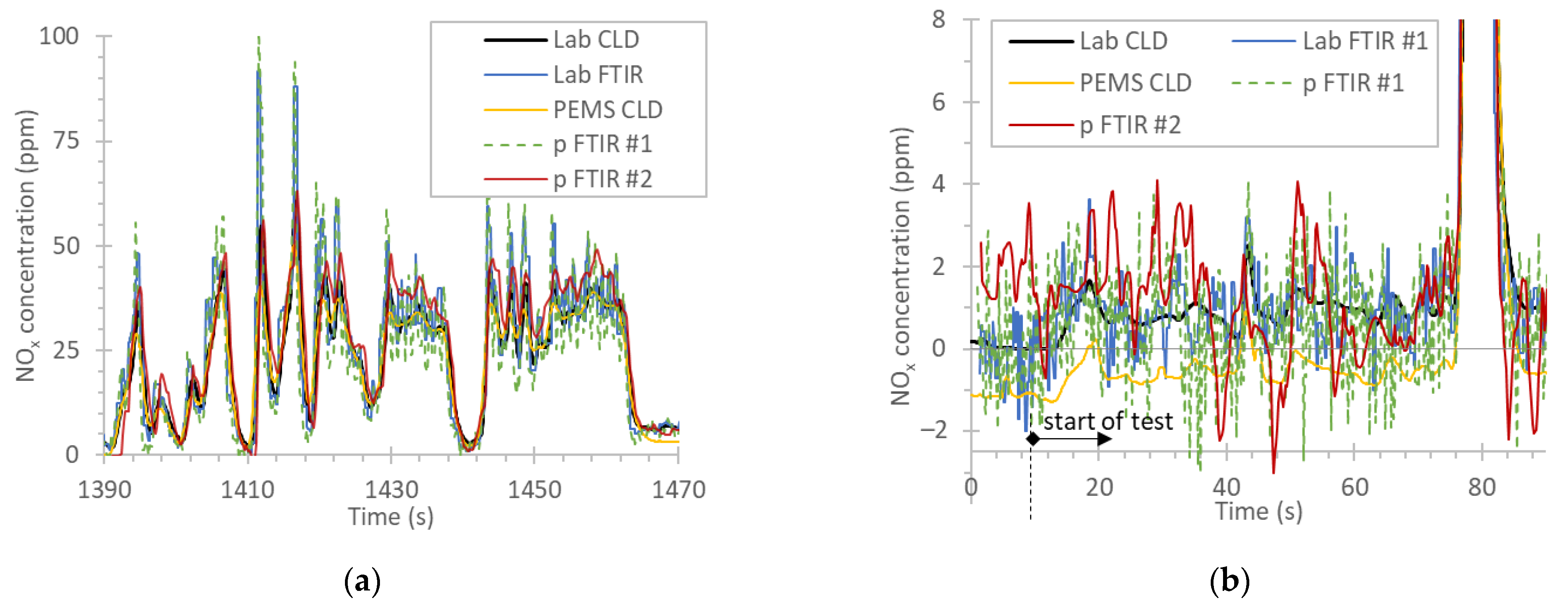
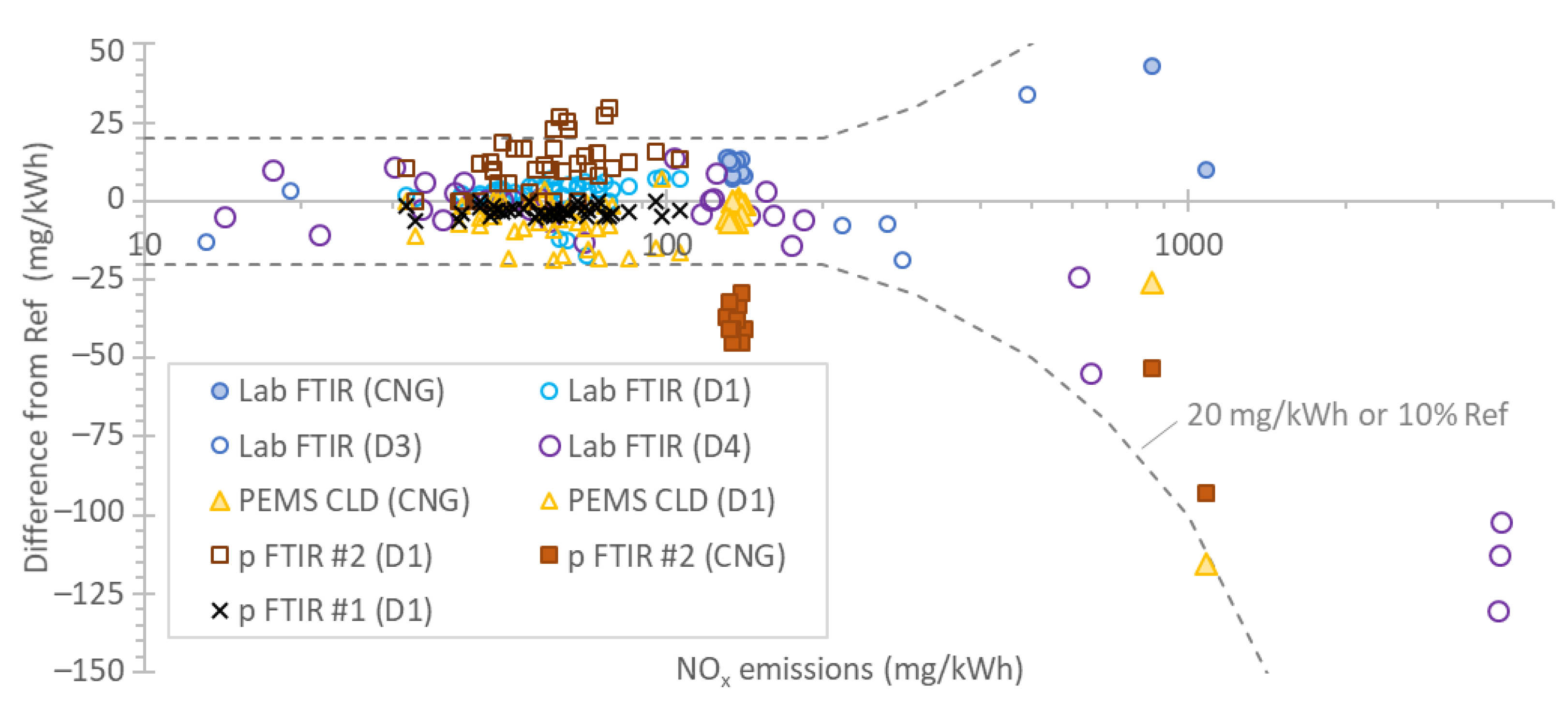
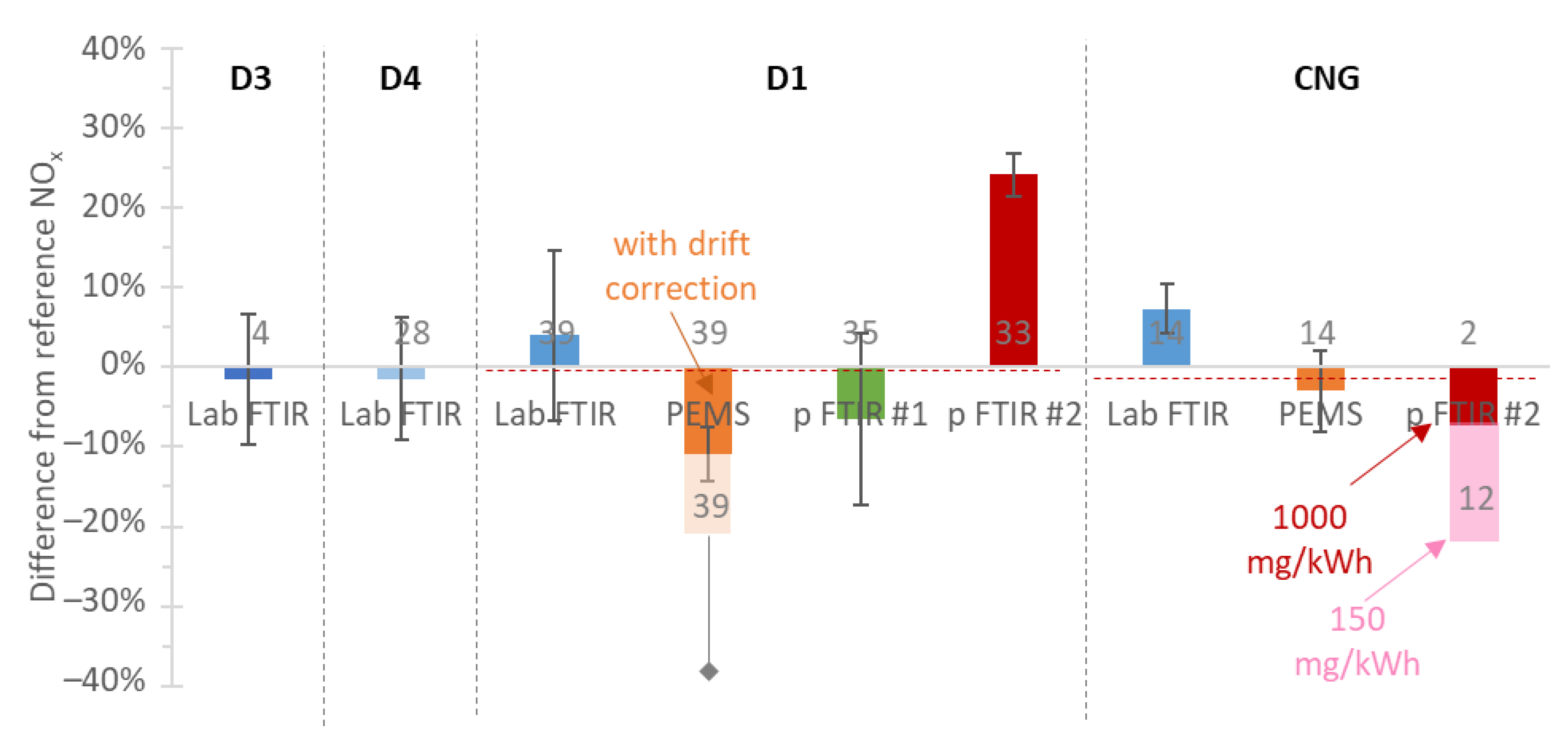
3.1. NOx
3.2. CO2
3.3. NH3
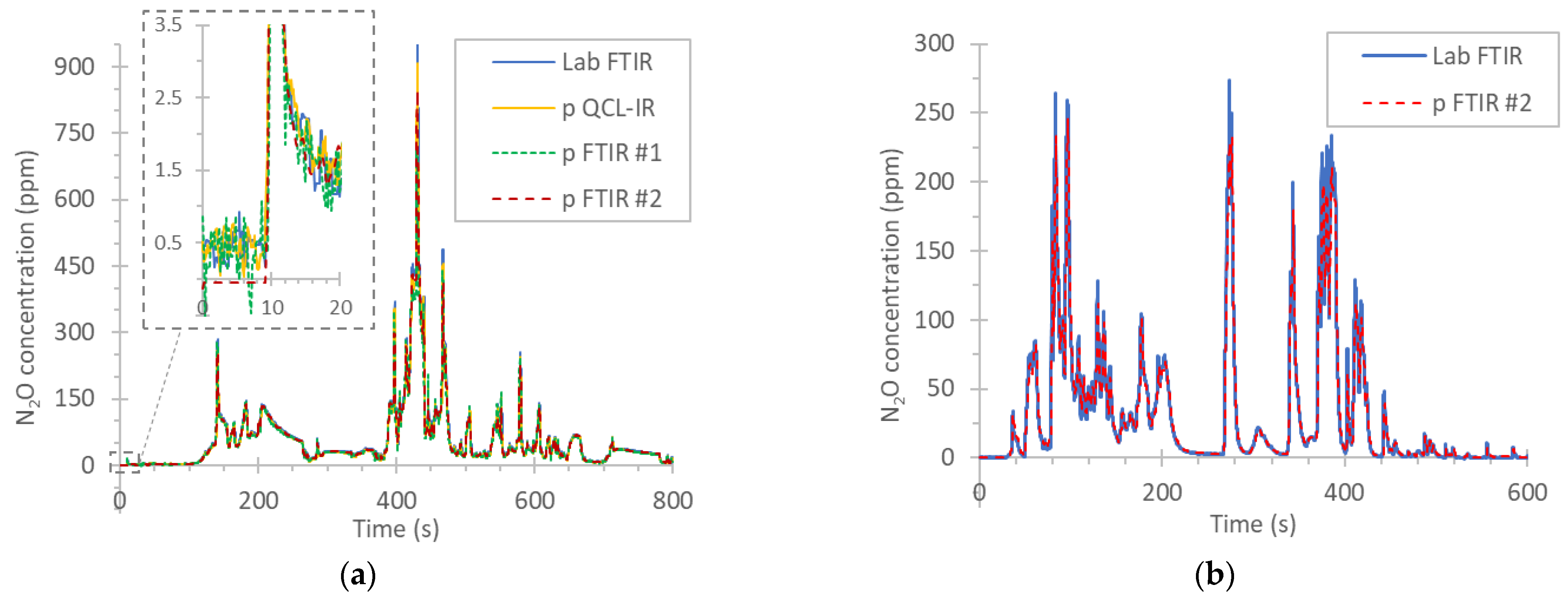
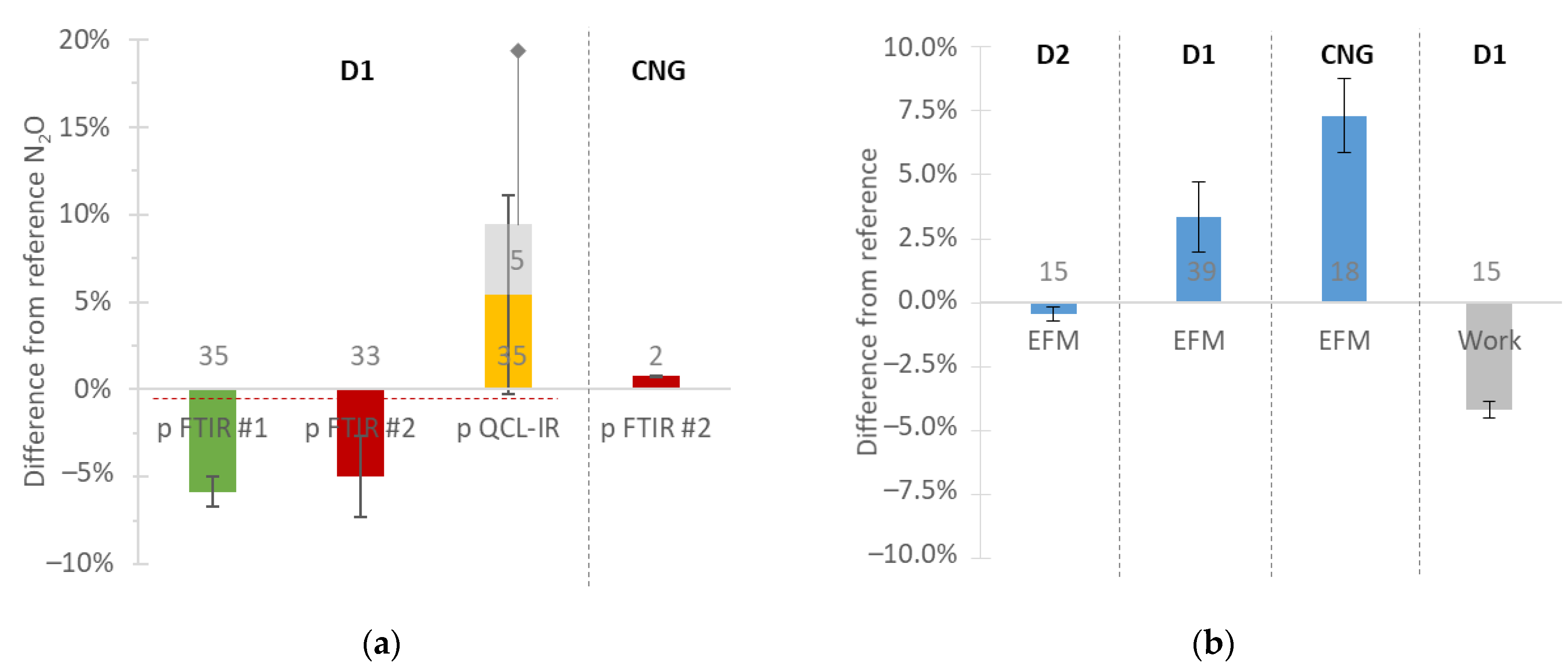
3.4. N2O
3.5. Exhaust Flow and Work
4. Discussion
- The uncertainty of the components that are needed for the calculation of the emissions (i.e., analyzer, exhaust flow, work) (see Equation (1));
- The uncertainty of the drift of the analyzers;
- The uncertainty of second-by-second measurements (dynamicity, time alignment);
- The impact of the boundary conditions (ambient temperature, altitude) on the instrument’s response.
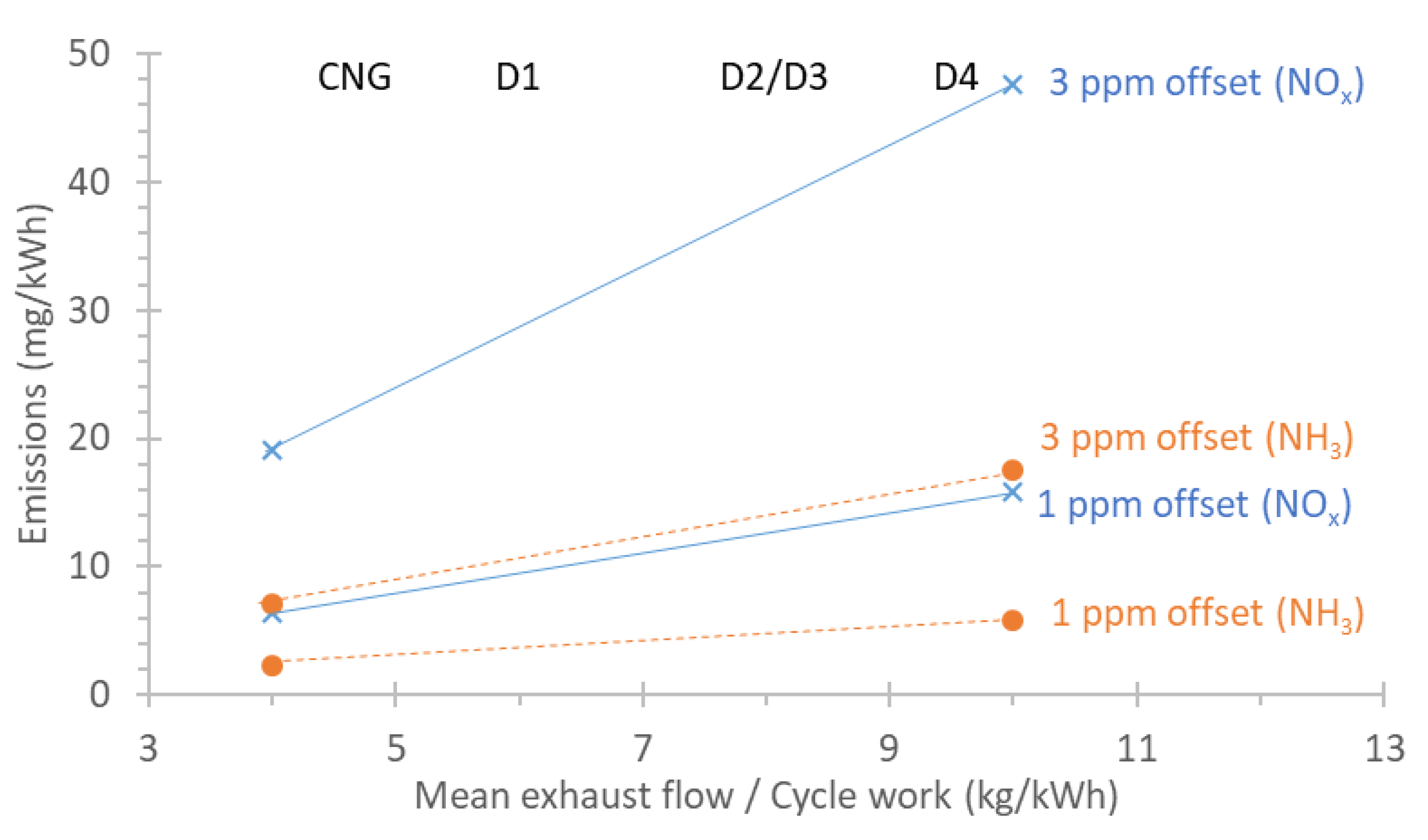
- A 1 ppm, NOx zero offset translates to 16 mg/kWh offset for a large ratio (10 kg/kWh), but 6 mg/kWh for a small ratio (4 kg/kWh);
- Higher offsets result in higher detection limits (proportionally). As a worst case (10 kg/kWh), a 3 ppm NOx zero offset is almost 50 mg/kWh offset;
- For NH3, the detection levels are almost three times lower due to the three times lower ugas.
5. Conclusions
Author Contributions
Funding
Institutional Review Board Statement
Informed Consent Statement
Data Availability Statement
Acknowledgments
Conflicts of Interest
Disclaimer
Appendix A

| Cycle | Ref CLD | Lab FTIR | PEMS | PEMS (Drift Corr.) | ||||
|---|---|---|---|---|---|---|---|---|
| Part | (ppm) | (mg/kWh) | (%)ppm | (%)mg/kWh | (%)ppm | (%)mg/kWh | (%)ppm | (%)mg/kWh |
| Low | 2.5 | 16.5 | 2% | 4% | −63% | −51% | −43% | −33% |
| High | 14.0 | 48.6 | 7% | 7% | −8% | −8% | −5% | −5% |
| WHTC | 4.6 | 70.8 | 5% | 6% | −33% | −20% | −22% | −13% |
| Cycle | Ref CLD | p FTIR #2 | p FTIR #1 | +0.6 s | −0.6 s | Smooth 3 s | ||
|---|---|---|---|---|---|---|---|---|
| Part | (mg/kWh) | (%)ppm | (%)mg/kWh | (%)ppm | (%)mg/kWh | (%)mg/kWh | (%)mg/kWh | (%)mg/kWh |
| Low | 16.5 | 12% | 20% | −7% | −13% | −15% | −11% | −13% |
| High | 48.6 | 13% | 14% | −1% | −2% | −4% | 0% | −2% |
| WHTC | 70.8 | 14% | 17% | −4% | −5% | −8% | −4% | −6% |
References
- Szymanski, P.; Ciuffo, B.; Fontaras, G.; Martini, G.; Pekar, F. The Future of Road Transport in Europe. Environmental Implications of Automated, Connected and Low-Carbon Mobility. Combust. Engines 2021, 186, 3–10. [Google Scholar] [CrossRef]
- Conway, G.; Joshi, A.; Leach, F.; García, A.; Senecal, P.K. A Review of Current and Future Powertrain Technologies and Trends in 2020. Transp. Eng. 2021, 5, 100080. [Google Scholar] [CrossRef]
- European Commission Reducing CO2 Emissions from Heavy-Duty Vehicles. 2019. Available online: https://ec.europa.eu/clima/eu-action/transport-emissions/road-transport-reducing-co2-emissions-vehicles/reducing-co2-emissions-heavy-duty-vehicles_en (accessed on 6 April 2022).
- Zhang, B.; Wu, S.; Cheng, S.; Lu, F.; Peng, P. Spatial Characteristics and Factor Analysis of Pollution Emission from Heavy-Duty Diesel Trucks in the Beijing–Tianjin–Hebei Region, China. Int. J. Environ. Res. Public Health 2019, 16, 4973. [Google Scholar] [CrossRef] [PubMed] [Green Version]
- Wang, X.; Song, G.; Zhai, Z.; Wu, Y.; Yin, H.; Yu, L. Effects of Vehicle Load on Emissions of Heavy-Duty Diesel Trucks: A Study Based on Real-World Data. Int. J. Environ. Res. Public Health 2021, 18, 3877. [Google Scholar] [CrossRef]
- Takeshita, T. Global Scenarios of Air Pollutant Emissions from Road Transport through to 2050. Int. J. Environ. Res. Public Health 2011, 8, 3032–3062. [Google Scholar] [CrossRef]
- Ethan, C.J.; Mokoena, K.K.; Yu, Y. Air Pollution Status in 10 Mega-Cities in China during the Initial Phase of the COVID-19 Outbreak. Int. J. Environ. Res. Public Health 2021, 18, 3172. [Google Scholar] [CrossRef]
- Song, X.; Hao, Y. Vehicular Emission Inventory and Reduction Scenario Analysis in the Yangtze River Delta, China. Int. J. Environ. Res. Public Health 2019, 16, 4790. [Google Scholar] [CrossRef] [Green Version]
- Clairotte, M.; Suarez-Bertoa, R.; Zardini, A.A.; Giechaskiel, B.; Pavlovic, J.; Valverde, V.; Ciuffo, B.; Astorga, C. Exhaust Emission Factors of Greenhouse Gases (GHGs) from European Road Vehicles. Environ. Sci. Eur. 2020, 32, 125. [Google Scholar] [CrossRef]
- Selleri, T.; Melas, A.D.; Joshi, A.; Manara, D.; Perujo, A.; Suarez-Bertoa, R. An Overview of Lean Exhaust DeNOx Aftertreatment Technologies and NOx Emission Regulations in the European Union. Catalysts 2021, 11, 404. [Google Scholar] [CrossRef]
- Giechaskiel, B.; Suarez-Bertoa, R.; Lahde, T.; Clairotte, M.; Carriero, M.; Bonnel, P.; Maggiore, M. Emissions of a Euro 6b Diesel Passenger Car Retrofitted with a Solid Ammonia Reduction System. Atmosphere 2019, 10, 180. [Google Scholar] [CrossRef] [Green Version]
- Bielaczyc, P.; Szczotka, A.; Woodburn, J. An Overview of Emissions of Reactive Nitrogen Compounds from Modern Light Duty Vehicles Featuring SI Engines. Combust. Engines 2014, 159, 48–53. [Google Scholar] [CrossRef]
- Woodburn, J. Emissions of Reactive Nitrogen Compounds (RNCs) from Two Vehicles with Turbo-Charged Spark Ignition Engines over Cold Start Driving Cycles. Combust. Engines 2021, 185, 3–9. [Google Scholar] [CrossRef]
- Updyke, K.M.; Nguyen, T.B.; Nizkorodov, S.A. Formation of Brown Carbon via Reactions of Ammonia with Secondary Organic Aerosols from Biogenic and Anthropogenic Precursors. Atmos. Environ. 2012, 63, 22–31. [Google Scholar] [CrossRef]
- Behera, S.N.; Sharma, M.; Aneja, V.P.; Balasubramanian, R. Ammonia in the Atmosphere: A Review on Emission Sources, Atmospheric Chemistry and Deposition on Terrestrial Bodies. Environ. Sci. Pollut. Res. 2013, 20, 8092–8131. [Google Scholar] [CrossRef]
- de Vries, W. Impacts of Nitrogen Emissions on Ecosystems and Human Health: A Mini Review. Curr. Opin. Environ. Sci. Health 2021, 21, 100249. [Google Scholar] [CrossRef]
- European Union. Euro 7 development. In Proceedings of the AGVES Advisory Group on Vehicle Emission Standards (AGVES), Brussels, Belgium, 31 March 2019. [Google Scholar]
- Kim, M.-K.; Park, D.; Kim, M.; Heo, J.; Park, S.; Chong, H. A Study on Characteristic Emission Factors of Exhaust Gas from Diesel Locomotives. Int. J. Environ. Res. Public Health 2020, 17, 3788. [Google Scholar] [CrossRef]
- Pang, K.; Zhang, K.; Ma, S. Tailpipe Emission Characterizations of Diesel-Fueled Forklifts under Real-World Operations Using a Portable Emission Measurement System. J. Environ. Sci. 2021, 100, 34–42. [Google Scholar] [CrossRef]
- Pang, K.; Zhang, K.; Ma, S.; Meng, X. Quantification of Emission Variability for Off-Road Equipment in China Based on Real-World Measurements. Front. Environ. Sci. Eng. 2021, 16, 24. [Google Scholar] [CrossRef]
- Wen, H.-T.; Lu, J.-H.; Jhang, D.-S. Features Importance Analysis of Diesel Vehicles’ NOx and CO2 Emission Predictions in Real Road Driving Based on Gradient Boosting Regression Model. Int. J. Environ. Res. Public Health 2021, 18, 13044. [Google Scholar] [CrossRef]
- Giechaskiel, B.; Clairotte, M.; Valverde-Morales, V.; Bonnel, P.; Kregar, Z.; Franco, V.; Dilara, P. Framework for the Assessment of PEMS (Portable Emissions Measurement Systems) Uncertainty. Environ. Res. 2018, 166, 251–260. [Google Scholar] [CrossRef]
- Giechaskiel, B.; Lähde, T.; Melas, A.D.; Valverde, V.; Clairotte, M. Uncertainty of Laboratory and Portable Solid Particle Number Systems for Regulatory Measurements of Vehicle Emissions. Environ. Res. 2021, 197, 111068. [Google Scholar] [CrossRef] [PubMed]
- Giechaskiel, B.; Bonnel, P.; Perujo, A.; Dilara, P. Solid Particle Number (SPN) Portable Emissions Measurement Systems (PEMS) in the European Legislation: A Review. Int. J. Environ. Res. Public Health 2019, 16, 4819. [Google Scholar] [CrossRef] [PubMed] [Green Version]
- Giechaskiel, B.; Lähde, T.; Gandi, S.; Keller, S.; Kreutziger, P.; Mamakos, A. Assessment of 10-Nm Particle Number (PN) Portable Emissions Measurement Systems (PEMS) for Future Regulations. Int. J. Environ. Res. Public Health 2020, 17, 3878. [Google Scholar] [CrossRef] [PubMed]
- Giechaskiel, B.; Clairotte, M. Fourier Transform Infrared (FTIR) Spectroscopy for Measurements of Vehicle Exhaust Emissions: A Review. Appl. Sci. 2021, 11, 7416. [Google Scholar] [CrossRef]
- Giechaskiel, B.; Suarez-Bertoa, R.; Lähde, T.; Clairotte, M.; Carriero, M.; Bonnel, P.; Maggiore, M. Evaluation of NOx Emissions of a Retrofitted Euro 5 Passenger Car for the Horizon Prize “Engine Retrofit”. Environ. Res. 2018, 166, 298–309. [Google Scholar] [CrossRef]
- Suarez-Bertoa, R.; Mendoza-Villafuerte, P.; Riccobono, F.; Vojtisek, M.; Pechout, M.; Perujo, A.; Astorga, C. On-Road Measurement of NH3 Emissions from Gasoline and Diesel Passenger Cars during Real World Driving Conditions. Atmos. Environ. 2017, 166, 488–497. [Google Scholar] [CrossRef]
- Vojtíšek-Lom, M.; Beránek, V.; Klír, V.; Jindra, P.; Pechout, M.; Voříšek, T. On-Road and Laboratory Emissions of NO, NO2, NH3, N2O and CH4 from Late-Model EU Light Utility Vehicles: Comparison of Diesel and CNG. Sci. Total Environ. 2018, 616–617, 774–784. [Google Scholar] [CrossRef]
- Mendoza-Villafuerte, P.; Suarez-Bertoa, R.; Giechaskiel, B.; Riccobono, F.; Bulgheroni, C.; Astorga, C.; Perujo, A. NOx, NH3, N2O and PN Real Driving Emissions from a Euro VI Heavy-Duty Vehicle. Impact of Regulatory on-Road Test Conditions on Emissions. Sci. Total Environ. 2017, 609, 546–555. [Google Scholar] [CrossRef]
- Suarez-Bertoa, R.; Mendoza-Villafuerte, P.; Bonnel, P.; Lilova, V.; Hill, L.; Perujo, A.; Astorga, C. On-Road Measurement of NH3 and N2O Emissions from a Euro V Heavy-Duty Vehicle. Atmos. Environ. 2016, 139, 167–175. [Google Scholar] [CrossRef]
- Varella, R.; Giechaskiel, B.; Sousa, L.; Duarte, G. Comparison of Portable Emissions Measurement Systems (PEMS) with Laboratory Grade Equipment. Appl. Sci. 2018, 8, 1633. [Google Scholar] [CrossRef] [Green Version]
- Suarez-Bertoa, R.; Zardini, A.A.; Lilova, V.; Meyer, D.; Nakatani, S.; Hibel, F.; Ewers, J.; Clairotte, M.; Hill, L.; Astorga, C. Intercomparison of Real-Time Tailpipe Ammonia Measurements from Vehicles Tested over the New World-Harmonized Light-Duty Vehicle Test Cycle (WLTC). Environ. Sci. Pollut. Res. 2015, 22, 7450–7460. [Google Scholar] [CrossRef] [PubMed] [Green Version]
- Suarez-Bertoa, R.; Clairotte, M.; Arlitt, B.; Nakatani, S.; Hill, L.; Winkler, K.; Kaarsberg, C.; Knauf, T.; Zijlmans, R.; Boertien, H.; et al. Intercomparison of Ethanol, Formaldehyde and Acetaldehyde Measurements from a Flex-Fuel Vehicle Exhaust during the WLTC. Fuel 2017, 203, 330–340. [Google Scholar] [CrossRef]
- Suarez-Bertoa, R.; Pechout, M.; Vojtíšek, M.; Astorga, C. Regulated and Non-Regulated Emissions from Euro 6 Diesel, Gasoline and CNG Vehicles under Real-World Driving Conditions. Atmosphere 2020, 11, 204. [Google Scholar] [CrossRef] [Green Version]
- Suarez-Bertoa, R.; Gioria, R.; Selleri, T.; Lilova, V.; Melas, A.; Onishi, Y.; Franzetti, J.; Forloni, F.; Perujo, A. NH3 and N2O Real World Emissions Measurement from a CNG Heavy Duty Vehicle Using On-Board Measurement Systems. Appl. Sci. 2021, 11, 10055. [Google Scholar] [CrossRef]
- Nakamura, H.; Kihara, N.; Adachi, M.; Ishida, K. Development of a Wet-Based NDIR and Its Application to on-Board Emission Measurement System; No. 2002-01-0612; SAE International: Warrendale, PA, USA, 2002. [Google Scholar]
- Nakamura, H.; Akard, M.; Porter, S.; Kihara, N.; Adachi, M.; Khalek, I.A. Performance Test Results of a New On Board Emission Measurement System Conformed with CFR Part 1065; No. 2007-01-1326; SAE International: Warrendale, PA, USA, 2007. [Google Scholar]
- Onishi, Y.; Hamauchi, S.; Shibuya, K.; McWilliams-Ward, K.; Akita, M.; Tsurumi, K. Development of On-Board NH3 and N2O Analyzer Utilizing Mid-Infrared Laser Absorption Spectroscopy; No. 2021-01-0610; SAE International: Warrendale, PA, USA, 2021. [Google Scholar]
- Shibuya, K.; Podzorov, A.; Matsuhama, M.; Nishimura, K.; Magari, M. High-Sensitivity and Low-Interference Gas Analyzer with Feature Extraction from Mid-Infrared Laser Absorption-Modulated Signal. Meas. Sci. Technol. 2021, 32, 035201. [Google Scholar] [CrossRef]
- Giakoumis, E.G. Driving and Engine Cycles; Springer: Cham, Switzerland, 2019; ISBN 978-3-319-84072-7. [Google Scholar]
- Giechaskiel, B.; Zardini, A.A.; Clairotte, M. Exhaust Gas Condensation during Engine Cold Start and Application of the Dry-Wet Correction Factor. Appl. Sci. 2019, 9, 2263. [Google Scholar] [CrossRef] [Green Version]
- Selleri, T.; Gioria, R.; Melas, A.D.; Giechaskiel, B.; Forloni, F.; Mendoza Villafuerte, P.; Demuynck, J.; Bosteels, D.; Wilkes, T.; Simons, O.; et al. Measuring Emissions from a Demonstrator Heavy-Duty Diesel Vehicle under Real-World Conditions—Moving Forward to Euro VII. Catalysts 2022, 12, 184. [Google Scholar] [CrossRef]
- Giechaskiel, B.; Valverde, V.; Clairotte, M. Real Driving Emissions (RDE): 2020 Assessment of Portable Emissions Measurement Systems (PEMS) Measurement Uncertainty; Publications Office of the European Union: Luxembourg, 2021; ISBN 978-92-76-30230-8. [Google Scholar]
- Giechaskiel, B.; Gioria, R.; Carriero, M.; Lähde, T.; Forloni, F.; Perujo, A.; Martini, G.; Bissi, L.M.; Terenghi, R. Emission Factors of a Euro VI Heavy-Duty Diesel Refuse Collection Vehicle. Sustainability 2019, 11, 1067. [Google Scholar] [CrossRef] [Green Version]
- Rahman, M.; Hara, K.; Nakatani, S.; Tanaka, Y. Development of a Fast Response Nitrogen Compounds Analyzer Using Quantum Cascade Laser for Wide-Range Measurement; No. 2011-26-0044; SAE International: Warrendale, PA, USA, 2011. [Google Scholar]
- Li, N.; El-Hamalawi, A.; Barrett, R.; Baxter, J. Ammonia Measurement Investigation Using Quantum Cascade Laser and Two Different Fourier Transform Infrared Spectroscopy Methods; No. 2020-01-0365; SAE International: Warrendale, PA, USA, 2020. [Google Scholar]
- Seykens, X.; van den Tillaart, E.; Lilova, V.; Nakatani, S. NH3 Measurements for Advanced SCR Applications; No. 2016-01-0975; SAE International: Warrendale, PA, USA, 2016. [Google Scholar]
- Ballantyne, V.F.; Howes, P.; Stephanson, L. Nitrous Oxide Emissions from Light Duty Vehicles; No. 940304; SAE International: Warrendale, PA, USA, 1994. [Google Scholar]
- Giechaskiel, B.; Casadei, S.; Mazzini, M.; Sammarco, M.; Montabone, G.; Tonelli, R.; Deana, M.; Costi, G.; Di Tanno, F.; Prati, M.; et al. Inter-Laboratory Correlation Exercise with Portable Emissions Measurement Systems (PEMS) on Chassis Dynamometers. Appl. Sci. 2018, 8, 2275. [Google Scholar] [CrossRef] [Green Version]
- Giechaskiel, B.; Casadei, S.; Rossi, T.; Forloni, F.; Di Domenico, A. Measurements of the Emissions of a “Golden” Vehicle at Seven Laboratories with Portable Emission Measurement Systems (PEMS). Sustainability 2021, 13, 8762. [Google Scholar] [CrossRef]
- Samaras, Z.; Andersson, J.; Aakko-Saksa, P.; Cuelenaere, R.; Mellios, G. Additional Technical Issues for Euro 7 (LDV). In Proceedings of the AGVES Meeting, (online). Webex, Brussels, Belgium, 24 February 2021. [Google Scholar]
- CEN/TS 17507:2021; Road Vehicles—Portable Emission Measuring Systems (PEMS)—Performance Assessment. BSI: London, UK, 2021.
- Zhang, K.; Frey, C. Evaluation of Response Time of a Portable System for In-Use Vehicle Tailpipe Emissions Measurement. Environ. Sci. Technol. 2008, 42, 221–227. [Google Scholar] [CrossRef] [PubMed]


| System | Portable | D1 | D2 | D3 | D4 | CNG |
|---|---|---|---|---|---|---|
| Lab analyzers | N | Y | Y | Y | Y | Y |
| Work (OBD) | Y | N | Y | N | N | N |
| EFM | Y | Y | Y | N | N | Y |
| PEMS | Y | Y | Y | N | N | Y |
| Lab FTIR | N | Y | N | Y | Y | Y |
| p FTIR #1 | Y | Y | N | N | N | N |
| p FTIR #2 | Y | Y | N | N | N | Y |
| p QCL-IR | Y | Y | N | N | N | N |
| Requirement | Lab Analyzers | Lab Analyzers | PEMS | Lab FTIR | p FTIR #1 | p FTIR #2 | p QCL-IR |
|---|---|---|---|---|---|---|---|
| Manufacturer | AVL | Horiba | Horiba | AVL | IAG | A&D | Horiba |
| Model | AMA i60 | MEXA-ONE | OBS-ONE | Sesam i60 | OFS | BOB-1000FT | OBS-ONE-XL |
| CO2 | NDIR | NDIR | Heated NDIR | Yes | Yes | Yes | - |
| NOx | CLD | CLD | CLD | Yes | Yes | Yes | - |
| N2O | - | - | - | Yes | Yes | Yes | Yes |
| NH3 | - | - | - | Yes | Yes | Yes | Yes |
| Sampling line | 6 m (191 °C) | 6 m (191 °C) | 6 m (191 °C) | 6 m (191 °C) | 6 m (191 °C) | 6 m (191 °C) | 6 m (113 °C) |
| t10–90 | ≤2.5 s | ≤2.5 s | ≤3.0 s | ≤3.0 s | ≤1.0 s | ≤2.0 s | ≤2.0 s |
| Qs (L/min) | 13 | 13 | 3 | 8 | 10 | 10 | 3.3 |
Publisher’s Note: MDPI stays neutral with regard to jurisdictional claims in published maps and institutional affiliations. |
© 2022 by the authors. Licensee MDPI, Basel, Switzerland. This article is an open access article distributed under the terms and conditions of the Creative Commons Attribution (CC BY) license (https://creativecommons.org/licenses/by/4.0/).
Share and Cite
Giechaskiel, B.; Jakobsson, T.; Karlsson, H.L.; Khan, M.Y.; Kronlund, L.; Otsuki, Y.; Bredenbeck, J.; Handler-Matejka, S. Assessment of On-Board and Laboratory Gas Measurement Systems for Future Heavy-Duty Emissions Regulations. Int. J. Environ. Res. Public Health 2022, 19, 6199. https://0-doi-org.brum.beds.ac.uk/10.3390/ijerph19106199
Giechaskiel B, Jakobsson T, Karlsson HL, Khan MY, Kronlund L, Otsuki Y, Bredenbeck J, Handler-Matejka S. Assessment of On-Board and Laboratory Gas Measurement Systems for Future Heavy-Duty Emissions Regulations. International Journal of Environmental Research and Public Health. 2022; 19(10):6199. https://0-doi-org.brum.beds.ac.uk/10.3390/ijerph19106199
Chicago/Turabian StyleGiechaskiel, Barouch, Tobias Jakobsson, Hua Lu Karlsson, M. Yusuf Khan, Linus Kronlund, Yoshinori Otsuki, Jürgen Bredenbeck, and Stefan Handler-Matejka. 2022. "Assessment of On-Board and Laboratory Gas Measurement Systems for Future Heavy-Duty Emissions Regulations" International Journal of Environmental Research and Public Health 19, no. 10: 6199. https://0-doi-org.brum.beds.ac.uk/10.3390/ijerph19106199