
A Deep Learning Method Approach for Sleep Stage Classification with EEG Spectrogram


Abstract
:1. Introduction
- An end-to-end classification method that uses only the spectrogram of a single channel EEG;
- Method yields superior overall accuracy in the unbalanced data, and good results for N1;
- The input size of the model used is fixed and there is no need to change the structure of the model or any of its parameters when a new set is used.
2. Materials and Methods
2.1. Datasets
2.1.1. Sleep-EDF and Sleep-EDFX
2.1.2. SHHS
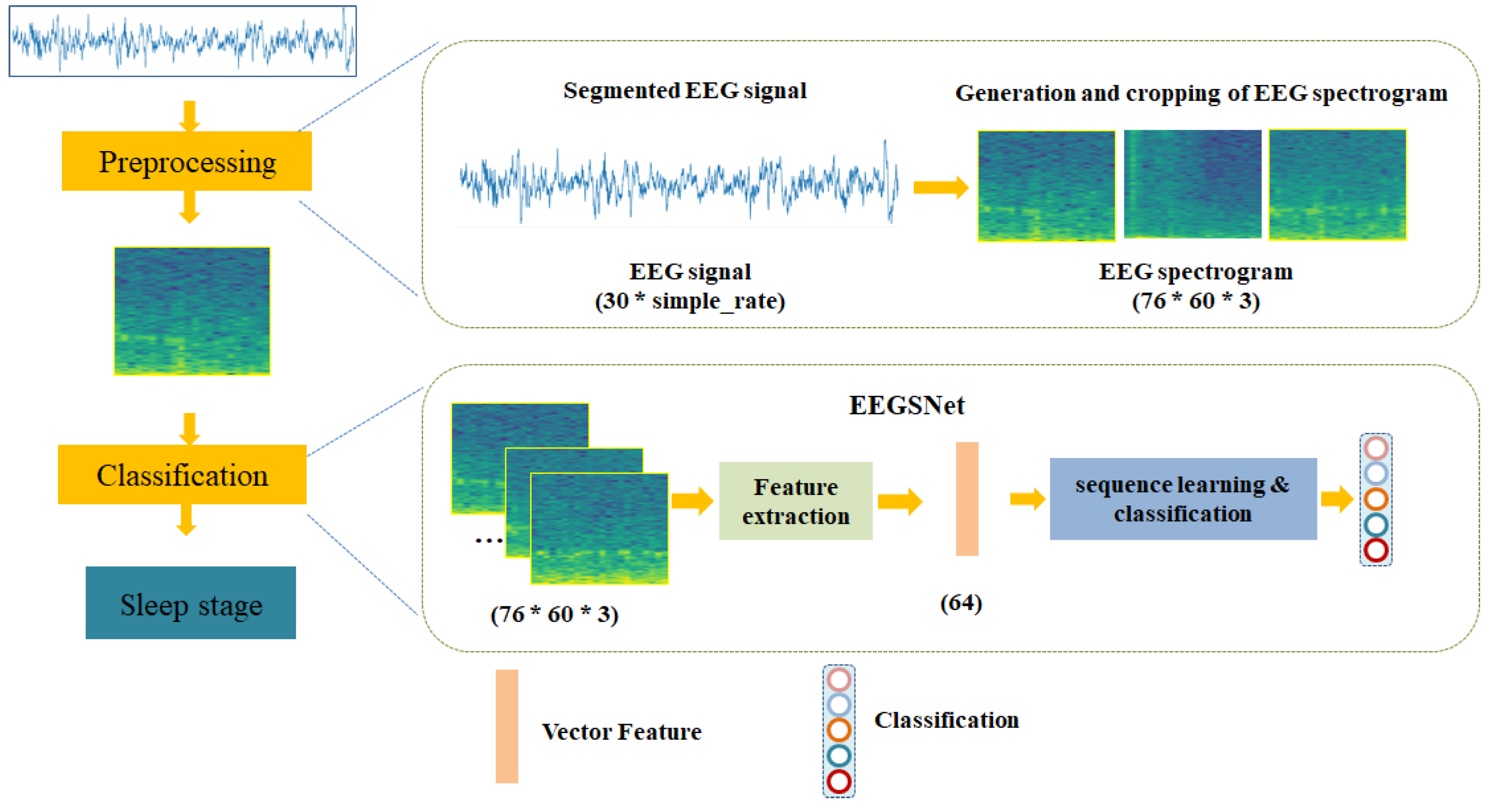
2.2. Methods
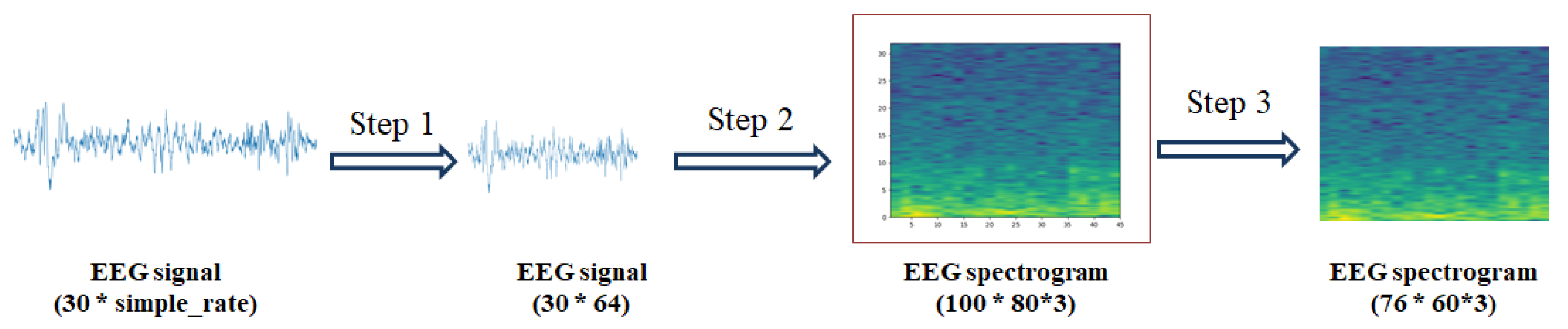
2.3. Preprocess
| Algorithm 1 The description of EEG spectrogram produce. |
| Input: EEG segment (Number of EEG segments n, Sample points per 30 s EEG segment p). Output: EEG spectrogram (Number of EEG segments n, Weight of spectrogram w, Height of spectrogram h, Channel of EEG spectrogram c). 1: Resample EEG signal into 64 Hz 2: Set spectrogram size = (1 ∗ 0.8) inches 3: for i = 0; i < n do 4: spctl1 = plt.specgram ( ) // Generate original size spectrogram. 5: spctl2 = spctl1 [14, 11, 90, 71] // Cut spctl1. The four numbers are the starting position of the abscissa and ordinate of image, and the ending position of the abscissa and ordinate. 6: end for |
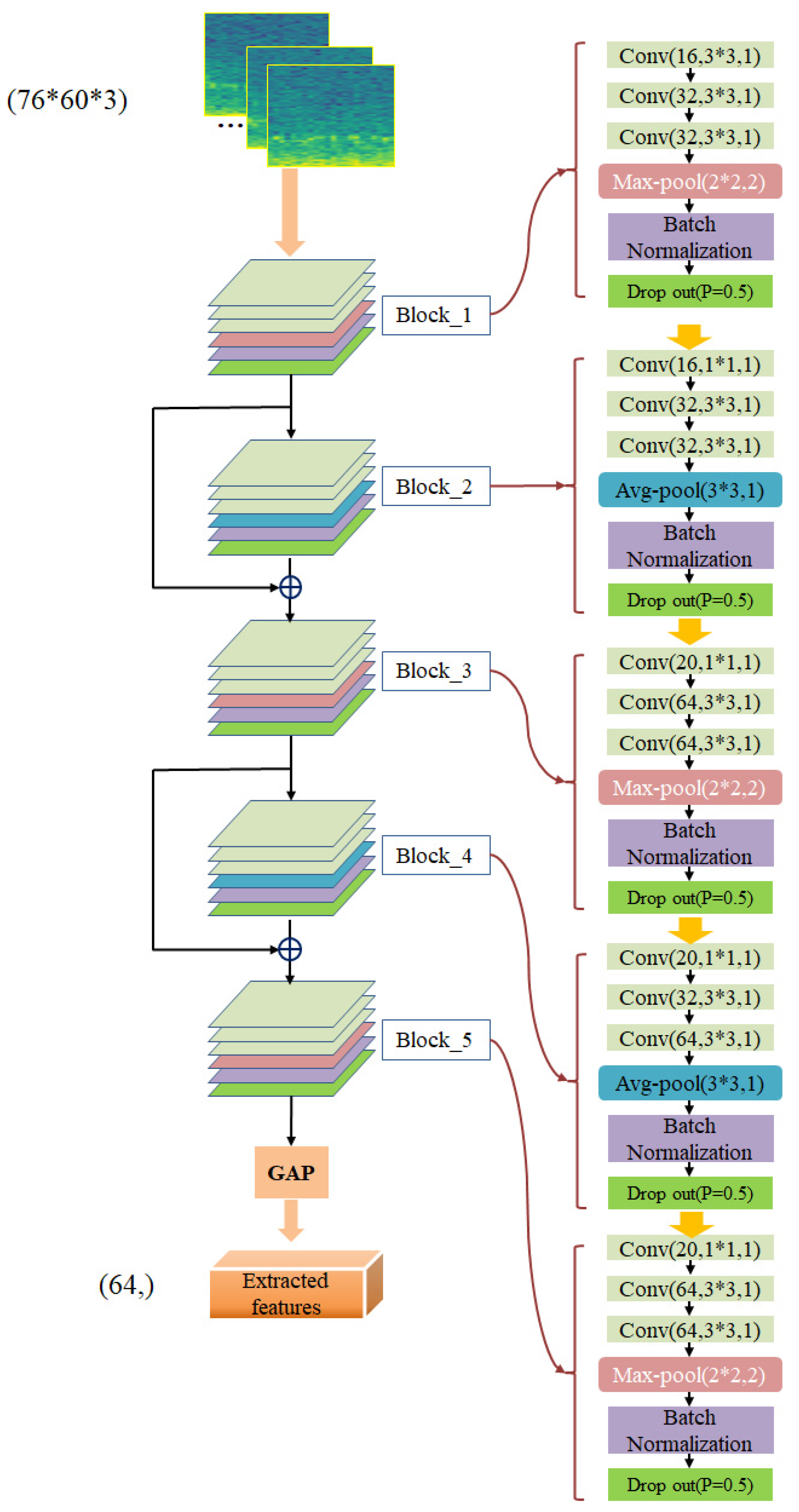
2.4. EEGSNet Model
2.4.1. Feature Extraction
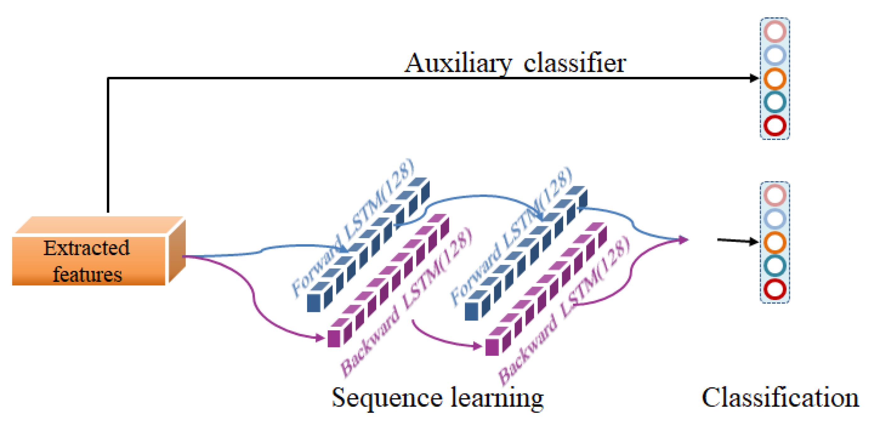
2.4.2. Sequence Learning
2.5. Training Detail
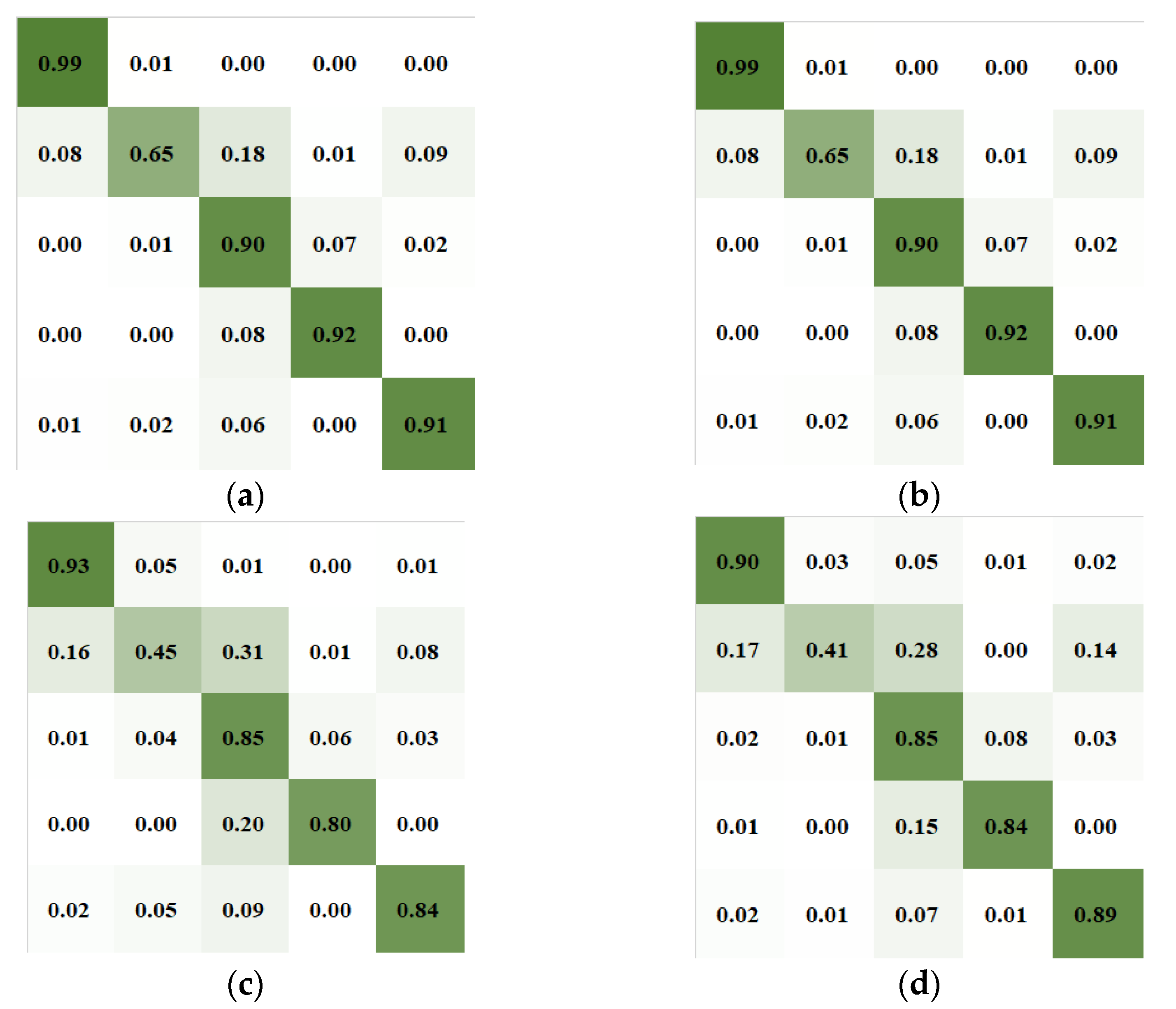
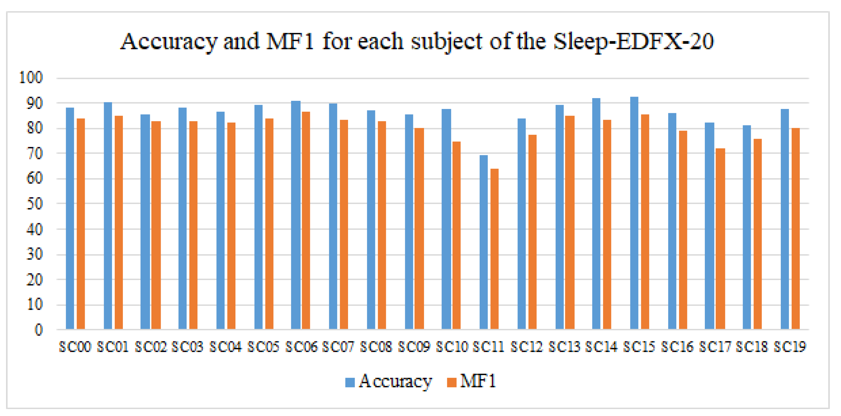
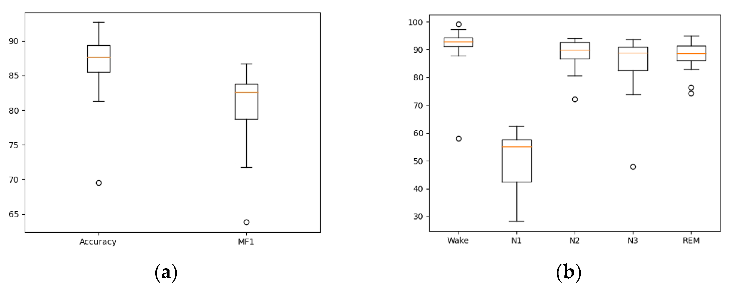
3. Results
Performance
4. Discussion
4.1. Comparison with Other Approaches
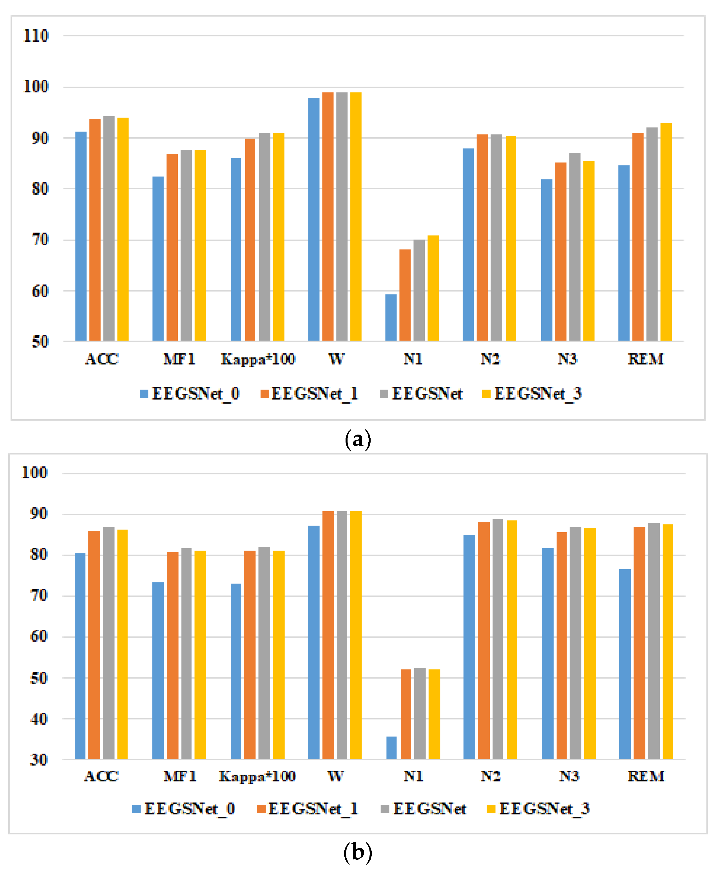
4.2. Ablation Experiments
- EEGSNet_0: EEGSNet without Bi-LSTM.
- EEGSNet_1: EEGSNet with one layer Bi-LSTM.
- EEGSNet_3: EEGSNet with three layers Bi-LSTM.
5. Conclusions
Author Contributions
Funding
Institutional Review Board Statement
Informed Consent Statement
Data Availability Statement
Acknowledgments
Conflicts of Interest
References
- Alickovic, E.; Subasi, A. Ensemble SVM method for automatic sleep stage classification. IEEE Trans. Instrum. Meas. 2018, 67, 1258–1265. [Google Scholar] [CrossRef] [Green Version]
- Rechtschaffen, A.; Kales, A. A Manual of Standardized Terminology, Techniques and Scoring System for Sleep Stages of Human Subjects; Brain Information Service/Brain Research Institute, University of California: Los Angeles, CA, USA, 1968. [Google Scholar]
- Iber, C.; Ancoli-Israel, S.; Chesson, A.; Quan, S. The AASM Manual for the Scoring of Sleep and Associated Events: Rules, Terminology and Technical Specifications; American Academy of Sleep Medicine: Westchester, IL, USA, 2007. [Google Scholar]
- Huang, Z.; Ling, B.W.-K. Sleeping stage classification based on joint quaternion valued singular spectrum analysis and ensemble empirical mode decomposition. Biomed. Signal Process. Control 2022, 71, 103086. [Google Scholar] [CrossRef]
- Shi, M.; Yang, C.; Zhang, D. A smart detection method of sleep quality using EEG signal and long short-term memory model. Math. Probl. Eng. 2021, 2021, 5515100. [Google Scholar] [CrossRef]
- Kuo, C.E.; Liang, S.F. Automatic stage scoring of single-channel sleep EEG based on multiscale permutation entropy. In Proceedings of the 2011 IEEE Biomedical Circuits and Systems Conference (BioCAS), San Diego, CA, USA, 10–12 November 2011; pp. 448–451. [Google Scholar]
- da Silveira, T.L.T.; Kozakevicius, A.J.; Rodrigues, C.R. Single-channel EEG sleep stage classification based on a streamlined set of statistical features in wavelet domain. Med. Biol. Eng. Comput. 2017, 55, 343–352. [Google Scholar] [CrossRef]
- Rahman, M.; Bhuiyan, M.I.H.; Hassan, A.R. Sleep stage classification using single-channel EOG. Comput. Biol. Med. 2018, 102, 211–220. [Google Scholar]
- Yang, Y.; Gao, Z.; Li, Y.; Wang, H. A CNN identified by reinforcement learning-based optimization framework for EEG-based state evaluation. J. Neural Eng. 2021, 18, 046059. [Google Scholar] [CrossRef]
- Yang, B.; Zhu, X.; Liu, Y.; Liu, H. A single-channel EEG based automatic sleep stage classification method leveraging deep one-dimensional convolutional neural network and hidden Markov model. Biomed. Signal Process. Control 2021, 68, 102581. [Google Scholar] [CrossRef]
- Wang, H.; Lu, C.; Zhang, Q.; Hu, Z.; Yuan, X.; Zhang, P.; Liu, W. A novel sleep staging network based on multi-scale dual attention. Biomed. Signal Process. Control 2022, 74, 103486. [Google Scholar] [CrossRef]
- Eldele, E.; Chen, Z.; Liu, C.; Wu, M.; Kwoh, C.K.; Li, X.; Guan, C. An attention-based deep learning approach for sleep stage classification with single-channel EEG. IEEE Trans. Neural Syst. Rehabil. Eng. 2021, 29, 809–818. [Google Scholar] [CrossRef]
- Mousavi, S.; Afghah, F.; Acharya, U.R. SleepEEGNet: Automated sleep stage scoring with sequence to sequence deep learning approach. PLoS ONE 2019, 14, e0216456. [Google Scholar] [CrossRef] [Green Version]
- Zhu, T.; Luo, W.; Yu, F. Convolution- and attention-based neural network for automated sleep stage classification. Int. J. Environ. Res. Public Health 2020, 17, 4152. [Google Scholar] [CrossRef] [PubMed]
- Huang, J.; Ren, L.; Zhou, X.; Yan, K. An improved neural network based on SENet for sleep stage classification. IEEE J. Biomed. Health Inform. 2022, 1. [Google Scholar] [CrossRef] [PubMed]
- Yulita, I.N.; Fanany, M.I.; Arymuthy, A.M. Bi-directional long short-term memory using quantized data of deep belief networks for sleep stage classification. Procedia Comput. Sci. 2017, 116, 530–538. [Google Scholar] [CrossRef]
- Yulita, I.N.; Fanany, M.I.; Arymurthy, A.M. Combining deep belief networks and bidirectional long short-term memory: Case study: Sleep stage classification. In Proceedings of the 2017 4th International Conference on Electrical Engineering, Computer Science and Informatics (EECSI), Yogyakarta, Indonesia, 19–21 September 2017; pp. 1–6. [Google Scholar]
- Supratak, A.; Dong, H.; Wu, C.; Guo, Y. DeepSleepNet: A model for automatic sleep stage scoring based on raw single-channel EEG. IEEE Trans. Neural Syst. Rehabil. Eng. 2017, 25, 1998–2008. [Google Scholar] [CrossRef] [PubMed] [Green Version]
- Seo, H.; Back, S.; Lee, S.; Park, D.; Kim, T.; Lee, K. Intra- and inter-epoch temporal context network (IITNet) using sub-epoch features for automatic sleep scoring on raw single-channel EEG. Biomed. Signal Process. Control 2020, 61, 102037. [Google Scholar] [CrossRef]
- Khalili, E.; Asl, B.M. Automatic sleep stage classification using temporal convolutional neural network and new data augmentation technique from raw single-channel EEG. Comput. Meth. Programs Biomed. 2021, 204, 106063. [Google Scholar] [CrossRef] [PubMed]
- Goldberger, A.L.; Amaral, L.; Glass, L.; Hausdorff, J.M.; Ivanov, P.; Mark, R.G.; Mietus, J.E.; Moody, G.B.; Peng, C.-K.; Stanley, H.E. The Sleep-EDF (Expanded) Database. 2000. Available online: https://physionet.org/content/sleep-edf/1.0.0/ (accessed on 12 December 2002).
- Goldberger, A.L.; Amaral, L.; Glass, J.; Hausdorff, J.M.; Ivanov, P.; Mark, R.G.; Mietus, J.E.; Moody, G.B.; Peng, C.-K.; Stanley, H.E. The Sleep-EDF (Expanded) Database. 2013. Available online: https://physionet.org/content/sleep-edfx/1.0.0/ (accessed on 24 October 2013).
- Zhang, G.-Q.; Cui, L.; Mueller, R.; Tao, S.; Kim, M.; Rueschman, M.; Mariani, S.; Mobley, D.; Redline, S. The national sleep research resource: Towards a sleep data commons. J. Am. Med. Inform. Assoc. 2018, 20, 1351–1358. [Google Scholar] [CrossRef] [Green Version]
- Hsu, Y.L.; Yang, Y.T.; Wang, J.S.; Hsu, C.Y. Automatic sleep stage recurrent neural classifier using energy features of EEG signals. Neurocomputing 2013, 104, 105–114. [Google Scholar] [CrossRef]
- Hassan, A.R.; Bhuiyan, M.I.H. An automated method for sleep staging from EEG signals using normal inverse Gaussian parameters and adaptive boosting. Neurocomputing 2017, 219, 76–87. [Google Scholar] [CrossRef]
- Schuster, M.; Paliwal, K.K. Bidirectional recurrent neural networks. IEEE Trans. Signal Process. 1997, 45, 2673–2681. [Google Scholar] [CrossRef] [Green Version]
- Phan, H.; Andreotti, F.; Cooray, N.; Chén, O.Y.; De Vos, M. SeqSleepNet: End-to-end hierarchical recurrent neural network for sequence-to-sequence automatic sleep staging. IEEE Trans. Neural Syst. Rehabil. Eng. 2019, 27, 400–410. [Google Scholar] [CrossRef] [PubMed] [Green Version]
- Supratak, A.; Guo, Y. TinySleepNet: An efficient deep learning model for sleep stage scoring based on raw single-channel EEG. In Proceedings of the 2020 42nd Annual International Conference of the IEEE Engineering in Medicine Biology Society (EMBC), Montreal, QC, Canada, 20–24 July 2020; pp. 641–644. [Google Scholar]
- Phan, H.; Chen, O.Y.; Tran, M.C.; Koch, P.; Mertins, A.; Vos, M.D. XSleepNet: Multi-view sequential model for automatic sleep staging. IEEE Trans. Pattern Anal. Mach. Intell. 2021, 1. [Google Scholar] [CrossRef] [PubMed]
- Sun, Y.; Wang, B.; Jin, J.; Wang, X. Deep convolutional network method for automatic sleep stage classification based on neurophysiological signals. In Proceedings of the 2018 11th International Congress on Image and Signal Processing, BioMedical Engineering and Informatics (CISP-BMEI), Beijing, China, 13–15 October 2018. [Google Scholar]
- Phan, H.; Andreotti, F.; Cooray, N.; Chén, O.Y.; De Vos, M. Joint classification and prediction CNN framework for automatic sleep stage classification. IEEE Trans. Biomed. Eng. 2019, 66, 1285–1296. [Google Scholar] [CrossRef] [PubMed]


| Dataset | Subjects | Wake | N1 | N2 | N3 | REM | Total |
|---|---|---|---|---|---|---|---|
| Sleep-EDFX-8 | 8 | 8037 | 604 | 3621 | 1299 | 1609 | 15,170 |
| Sleep-EDFX-20 | 20 | 8285 | 2804 | 17,799 | 5703 | 7717 | 42,308 |
| Sleep-EDFX-78 | 78 | 65,951 | 21,522 | 69,132 | 13,039 | 25,835 | 195,479 |
| SHHS | 329 | 46,319 | 10,304 | 142,125 | 60,153 | 65,953 | 324,854 |
| Dataset | Wake-N1 | Wake-REM | N1–N2 | REM-N2 |
|---|---|---|---|---|
| Sleep-EDFX-8 | 95 | 0 | 157 | 14 |
| Sleep-EDFX-20 | 442 | 32 | 688 | 136 |
| Sleep-EDFX-78 | 3988 | 86 | 4269 | 427 |
| SHHS | 4615 | 623 | 3585 | 869 |
| Stage | Predicted | Per-Class Metrics | ||||||
|---|---|---|---|---|---|---|---|---|
| Wake | N1 | N2 | N3 | REM | PR (%) | RE (%) | F1 (%) | |
| W | 7873 | 46 | 13 | 7 | 6 | 99.1 | 99.1 | 99.1 |
| N1 | 50 | 388 | 105 | 4 | 52 | 76.5 | 64.8 | 70.2 |
| N2 | 8 | 49 | 3230 | 234 | 55 | 91.0 | 90.3 | 90.7 |
| N3 | 3 | 0 | 104 | 1191 | 1 | 82.8 | 91.7 | 87.0 |
| REM | 14 | 24 | 96 | 3 | 1444 | 92.7 | 91.3 | 90.0 |
| Stage | Predicted | Per-Class Metrics | ||||||
|---|---|---|---|---|---|---|---|---|
| Wake | N1 | N2 | N3 | REM | PR (%) | RE (%) | F1 (%) | |
| W | 7585 | 291 | 102 | 20 | 88 | 89.8 | 93.8 | 91.76 |
| N1 | 363 | 1291 | 673 | 12 | 429 | 59.8 | 46.6 | 52.41 |
| N2 | 336 | 382 | 15,596 | 741 | 554 | 89 | 88.6 | 88.78 |
| N3 | 29 | 1 | 663 | 4914 | 2 | 86.4 | 87.6 | 87 |
| REM | 133 | 194 | 491 | 0 | 6860 | 86.5 | 89.3 | 87.89 |
| Stage | Predicted | Per-Class Metrics | ||||||
|---|---|---|---|---|---|---|---|---|
| Wake | N1 | N2 | N3 | REM | PR (%) | RE (%) | F1 (%) | |
| W | 61,212 | 3406 | 506 | 44 | 462 | 93.1 | 93.3 | 93.2 |
| N1 | 3359 | 9744 | 6568 | 133 | 1683 | 55.8 | 45.3 | 50.0 |
| N2 | 539 | 3097 | 58,825 | 4259 | 2276 | 83.2 | 85.3 | 84.2 |
| N3 | 20 | 22 | 2580 | 10,360 | 8 | 69.7 | 79.8 | 74.4 |
| REM | 608 | 1199 | 2263 | 59 | 21,618 | 83.0 | 84.0 | 83.5 |
| Stage | Predicted | Per-Class Metrics | ||||||
|---|---|---|---|---|---|---|---|---|
| Wake | N1 | N2 | N3 | REM | PR (%) | RE (%) | F1 (%) | |
| W | 41,458 | 1222 | 2261 | 260 | 900 | 87.2 | 89.9 | 88.6 |
| N1 | 1706 | 4221 | 2857 | 24 | 1460 | 55.6 | 41.1 | 47.3 |
| N2 | 2397 | 1534 | 120,994 | 11,945 | 4725 | 86.5 | 85.5 | 86.0 |
| N3 | 409 | 2 | 8896 | 50,471 | 230 | 80.1 | 84.1 | 82.0 |
| REM | 1562 | 615 | 4824 | 346 | 58,481 | 88.9 | 88.8 | 88.9 |
| Methods | Epochs | Overall Metrics | Per-Class F1 | ||||||
|---|---|---|---|---|---|---|---|---|---|
| ACC | MF1 | Kappa | W | N1 | N2 | N3 | REM | ||
| Ref. [4] | 15,199 | 90.66 | 76.33 | 0.85 | 97.60 | 31.2 | 88.17 | 84.03 | 80.65 |
| Ref. [11] | 15,199 | 91.74 | 82.31 | 0.87 | 98.51 | 54.41 | 89.73 | 86.47 | 82.42 |
| Ref. [27] | 15,188 | 93.7 | 84.5 | 0.90 | 98.6 | 52.5 | 92.1 | 87.3 | 91.80 |
| EEGSNet | 15,170 | 94.17 | 87.78 | 0.91 | 99.08 | 70.16 | 90.68 | 87.00 | 92.00 |
| Methods | Param | Epochs | Overall Metrics | Per-Class F1 | ||||||
|---|---|---|---|---|---|---|---|---|---|---|
| ACC | MF1 | Kappa | W | N1 | N2 | N3 | REM | |||
| 1D-CNN-HMM [10] | - | 42,308 | 83.98 | 76.9 | 0.78 | 87.8 | 35.1 | 86.6 | 90.5 | 86.8 |
| Ref. [9] | - | 42,309 | 84 | 75.2 | 0.78 | 89.4 | 30.3 | 88.5 | 89.2 | 78.4 |
| Ref. [20] | - | 41,950 | 85.39 | 79.27 | 0.8 | 90.5 | 46.6 | 88.4 | 86.1 | 84.6 |
| AttnSleep [12] | - | 42,308 | 84.4 | 78.1 | 0.79 | 89.7 | 42.6 | 88.8 | 90.2 | 79 |
| Ref. [14] | - | 42,269 | 82.83 | 77.8 | 0.77 | 90.3 | 47.1 | 86.0 | 82.1 | 83.2 |
| IITNet [19] | - | 42,308 | 83.6 | 76.5 | 0.77 | 87.1 | 39.2 | 87.7 | 87.7 | 80.9 |
| SleepEEGNet [13] | 2.6 M | 42,308 | 84.26 | 79.66 | 0.79 | 89.19 | 52.19 | 86.77 | 85.13 | 85.02 |
| DeepSleepNet [18] | 24.7 M | 41,950 | 82 | 76.9 | 0.76 | 84.7 | 46.6 | 85.9 | 84.8 | 82.4 |
| SeqSleepNet+ [27] | 0.2 M | 42,308 | 85.2 | 78.4 | 0.80 | 90.5 | 45.4 | 88.1 | 86.4 | 81.8 |
| TinySleepNet [28] | 1.3 M | 42,308 | 85.4 | 80.5 | 0.80 | 90.1 | 51.4 | 88.5 | 88.3 | 84.3 |
| XSleepNet [29] | 5.8 M | 42,308 | 86.3 | 80.6 | 0.81 | 90.2 | 51.8 | 88.0 | 86.8 | 83.9 |
| EEGSNet | 0.6 M | 42,308 | 86.82 | 81.57 | 0.82 | 90.76 | 52.41 | 88.78 | 87.0 | 87.89 |
| Methods | Epochs | Overall Metrics | Per-Class F1 | ||||||
|---|---|---|---|---|---|---|---|---|---|
| ACC | MF1 | Kappa | W | N1 | N2 | N3 | REM | ||
| SleepEEGNet [13] | 222,479 | 80.03 | 73.55 | 0.73 | 91.72 | 44.05 | 82.49 | 73.45 | 76.06 |
| AttnSleep [12] | 195,479 | 81.3 | 75.1 | 0.74 | 92.0 | 42.0 | 85.0 | 82.1 | 74.2 |
| Ref. [20] | 191,585 | 82.46 | 76.14 | 0.76 | 92.4 | 48.1 | 84.6 | 73.8 | 81.6 |
| EEGSNet | 195,479 | 83.02 | 77.26 | 0.77 | 93.19 | 50.03 | 84.19 | 74.41 | 83.48 |
| Methods | Epochs | Overall Metrics | Per-Class F1 | ||||||
| ACC | MF1 | Kappa | W | N1 | N2 | N3 | REM | ||
| DeepSleepNet [18] | 324,854 | 81.0 | 73.9 | 0.73 | 85.4 | 40.5 | 82.5 | 79.3 | 81.9 |
| SleepEEGNet [13] | 324,854 | 73.9 | 68.4 | 0.65 | 81.3 | 34.4 | 73.4 | 75.9 | 77.0 |
| ResnetLSTM [30] | 324,854 | 83.3 | 69.4 | 0.76 | 85.1 | 9.4 | 86.3 | 87.0 | 79.1 |
| multitaskCNN [31] | 324,854 | 81.4 | 71.2 | 0.74 | 82.2 | 25.7 | 83.9 | 83.3 | 81.1 |
| AttnSleep [12] | 324,854 | 84.2 | 75.3 | 0.78 | 86.7 | 33.2 | 87.1 | 87.1 | 82.1 |
| EEGSNet | 324,854 | 85.12 | 78.54 | 0.79 | 88.55 | 47.26 | 85.99 | 82.03 | 88.86 |
Publisher’s Note: MDPI stays neutral with regard to jurisdictional claims in published maps and institutional affiliations. |
© 2022 by the authors. Licensee MDPI, Basel, Switzerland. This article is an open access article distributed under the terms and conditions of the Creative Commons Attribution (CC BY) license (https://creativecommons.org/licenses/by/4.0/).
Share and Cite
Li, C.; Qi, Y.; Ding, X.; Zhao, J.; Sang, T.; Lee, M. A Deep Learning Method Approach for Sleep Stage Classification with EEG Spectrogram. Int. J. Environ. Res. Public Health 2022, 19, 6322. https://0-doi-org.brum.beds.ac.uk/10.3390/ijerph19106322
Li C, Qi Y, Ding X, Zhao J, Sang T, Lee M. A Deep Learning Method Approach for Sleep Stage Classification with EEG Spectrogram. International Journal of Environmental Research and Public Health. 2022; 19(10):6322. https://0-doi-org.brum.beds.ac.uk/10.3390/ijerph19106322
Chicago/Turabian StyleLi, Chengfan, Yueyu Qi, Xuehai Ding, Junjuan Zhao, Tian Sang, and Matthew Lee. 2022. "A Deep Learning Method Approach for Sleep Stage Classification with EEG Spectrogram" International Journal of Environmental Research and Public Health 19, no. 10: 6322. https://0-doi-org.brum.beds.ac.uk/10.3390/ijerph19106322