Long- and Short-Term Cryptocurrency Volatility Components: A GARCH-MIDAS Analysis

Abstract

We use the GARCH-MIDAS model to extract the long- and short-term volatility components of cryptocurrencies. As potential drivers of Bitcoin volatility, we consider measures of volatility and risk in the US stock market as well as a measure of global economic activity. We find that S&P 500 realized volatility has a negative and highly significant effect on long-term Bitcoin volatility. The finding is atypical for volatility co-movements across financial markets. Moreover, we find that the S&P 500 volatility risk premium has a significantly positive effect on long-term Bitcoin volatility. Finally, we find a strong positive association between the Baltic dry index and long-term Bitcoin volatility. This result shows that Bitcoin volatility is closely linked to global economic activity. Overall, our findings can be used to construct improved forecasts of long-term Bitcoin volatility.

“After Lehman Brothers toppled in September 2008, it took 24 days for US stocks to slide more than 20 per cent into official bear market territory. Bitcoin, the new age cryptocurrency that has been breaking bull market records, did the same on Wednesday in just under six hours”

Financial Times—30 November 2017—Bitcoin swings from bull to bear and back in one day

1. Introduction

Bitcoin is surely not short on publicity as its rise, subsequent decline and volatile swings have drawn the attention from academics and business leaders alike. There are many critics. For example, Nobel laureate Joseph Stiglitz said that Bitcoin ought to be outlawed whereas fellow Nobel laureate Robert Shiller said the currency appeals to some investors because it has an anti-government, anti-regulation feel. Many business leaders, including Carl Icahn and Warren Buffett, characterized its spectacular price increases as a bubble. Jamie Dimon, CEO of JP Morgan called it a fraud, and implicitly alluding to bubbles that ultimately burst, predicted that it eventually would blow up. Along similar lines, Goldman Sachs CEO Lloyd Blankfein is on the record for saying that the currency serves as a vehicle for perpetrating fraud, although he acknowledged that the currency could have potential if volatility drops.

Cryptocurrencies has its defenders and enthusiasts as well. The CME Group listed Bitcoin futures in mid-December 2017 and Nasdaq plans to launch Bitcoin futures this year. The currency also has many supporters in Silicon Valley. The listing of Bitcoin futures and the proliferation of cryptocurrencies in general has generated a growing literature on the topic.

Most of the existing studies focus on Bitcoin returns. For example, Baur et al. (2017) show that Bitcoin returns are essentially uncorrelated with traditional asset classes such as stocks or bonds, which points to diversification possibilities. Others investigate the determinants of Bitcoin returns. The findings of Li and Wang (2017), among others, suggest that measures of financial and macroeconomic activity are drivers of Bitcoin returns. Kristoufek (2015) considers financial uncertainty, Bitcoin trading volume in Chinese Yuan and Google trends as potential drivers of Bitcoin returns. The inclusion of Google trends as some sort of proxy for sentiment or interest is fairly common within the literature (see, for example, Polasik et al. (2015)). A recurrent theme in the literature is the question to which asset class Bitcoin belongs, with many comparing it to gold, others to precious metals or to speculative assets (see, among others, Baur et al. (2017); or Bouri et al. (2017)). Some have classified Bitcoin as something in between a currency and a commodity (see, for example, Dyhrberg (2016)). For other recent contributions, see Cheah et al. (2018); Khuntia and Pattanayak (2018); and Koutmos (2018).

A second strand of literature tries to model Bitcoin volatility. Among the first papers is Balcilar et al. (2017), who analyze the causal relation between trading volume and Bitcoin returns and volatility. They find that volume cannot help predict the volatility of Bitcoin returns. Dyhrberg (2016) explores Bitcoin volatility using GARCH models. The models estimated in Dyhrberg (2016) suggest that Bitcoin has several similarities with both gold and the dollar. Bouri et al. (2017) find no evidence for asymmetry in the conditional volatility of Bitcoins when considering the post December 2013 period and investigate the relation between the VIX index and Bitcoin volatility. Al-Khazali et al. (2018) consider a model for daily Bitcoin returns and show that Bitcoin volatility tends to decrease in response to positive news about the US economy. Finally, Katsiampa (2017) explores the applicability of several ARCH-type specifications to model Bitcoin volatility and selects an AR-CGARCH model as the preferred specification. Although Katsiampa (2017) suggests that Bitcoin volatility consists of long- and short-term components, he does not investigate the determinants of Bitcoin volatility.

We use the GARCH-MIDAS model of Engle et al. (2013) for investigating the economic determinants of long-term Bitcoin volatility. While all the previous studies considered Bitcoin returns/volatility as well as their potential determinants at the same (daily) frequency, the MIxed Data Sampling (MIDAS) technique offers a unique framework to investigate macroeconomic and financial variables that are sampled at a lower (monthly) frequency than the Bitcoin returns as potential drivers of Bitcoin volatility. Specifically, the two-component GARCH-MIDAS model consists of a short-term GARCH component and a long-term component. The model allows explanatory variables to enter directly into the specification of the long-term component.

As potential drivers of Bitcoin volatility, we consider macroeconomic and financial variables, such as the Baltic dry index and the VIX, but also Bitcoin specific variables, such as trading volume. In addition, we analyze the drivers of the volatility of the S&P 500, the Nikkei 225, gold and copper. This allows for a comparison of the effects on the different assets and provides further useful insights for a classification of Bitcoin as an asset class.

Our main findings can be summarized as follows: First, Bitcoin volatility is negatively related to US stock market volatility. This observation is consistent with investors who consider Bitcoin as a safe-haven. Second, in contrast to stock market volatility, Bitcoin volatility behaves pro-cyclical, i.e., increases with higher levels of global economic activity. Third, the response of Bitcoin volatility to higher levels of US stock market volatility is the opposite of the response of gold volatility. This questions the meaningfulness of comparisons between Bitcoin and gold. Finally, while most previous studies focused on short-term relationships using exclusively daily data, our results highlight the importance of also investigating the relationship between long-term Bitcoin volatility and its economic drivers.

In Section 2, we introduce the GARCH-MIDAS model as it is applied in the current setting. Section 3 describes the data. The empirical results are presented in Section 4. Section 5 concludes the paper.

2. Model

We model Bitcoin volatility as a GARCH-MIDAS processs. Engle et al. (2013) discuss the technical details of this class of models where the conditional variance is multiplicatively decomposed into a short-term (high-frequency) and a long-term (low-frequency) component. The long-term component is expressed as a function of observable explanatory variables. This allows us to investigate the financial and macroeconomic determinants of Bitcoin volatility. In the empirical application, we consider daily Bitcoin returns and monthly explanatory variables.

We define daily Bitcoin returns as $r_{i,t}=100·(ln(P_{i,t}-ln\left(P_{i-1,t}\right))$, where $t=1,\dots ,T$ denotes the monthly frequency and $i=1,\dots ,N_t$ the number of days within month t. We assume that the conditional mean of Bitcoin returns is constant, i.e.,

$$r_{i,t}=\mu +{\epsilon }_{i,t},$$

(1)

with

$${\epsilon }_{i,t}=\sqrt{h_{i,t}{\tau }_t}{Z}_{i,t}.$$

(2)

The innovation $Z_{i,t}$ is assumed to be i.i.d. with mean zero and variance one. $h_{i,t}$ and ${\tau }_t$ denote the short- and long-term component of the conditional variance, respectively. The short-term component $h_{i,t}$ varies at the daily frequency and follows a unit-variance GARCH(1,1) process

$$h_{i,t}=(1-\alpha -\beta )+\alpha \frac{{\epsilon }_{i-1,t}^2}{{\tau }_t}+\beta h_{i-1,t},$$

(3)

where $\alpha >0$, $\beta \ge 0$ and $\alpha +\beta <1$. The long-term component varies at the monthly frequency and is given by

$${\tau }_t=m+\sum _{k=1}^K{\phi }_k({\omega }_1,{\omega }_2)X_{t-k},$$

(4)

where $X_t$ denotes the explanatory variable and ${\phi }_k({\omega }_1,{\omega }_2)$ a certain weighting scheme. We opt for the Beta weighting scheme, which is given by

$${\phi }_k({\omega }_1,{\omega }_2)=\frac{{\left(k/(K+1)\right)}^{{\omega }_1-1}·{\left(1-k/(K+1)\right)}^{{\omega }_2-1}}{{\sum }_{j=1}^K{\left(j/(K+1)\right)}^{{\omega }_1-1}·{\left(1-j/(K+1)\right)}^{{\omega }_2-1}}.$$

(5)

By construction, the weights ${\phi }_k({\omega }_1,{\omega }_2)\ge 0$, $k=1,\dots ,K$, sum to one. In the empirical application, we impose the restriction that ${\omega }_1=1$, which implies that the weights are monotonically declining. Following Conrad and Loch (2015), we employ three MIDAS lag years, i.e., we choose $K=36$ for the monthly explanatory variables. Our empirical results show that this choice is appropriate in the sense that the estimated weights approach zero before lag 36. As in Engle et al. (2013), we estimate the GARCH-MIDAS models by quasi-maximum likelihood and construct heteroscedasticity and autocorrelation consistent (HAC) standard errors.

3. Data

Our analysis utilizes cryptocurrency specific data, measures of financial conditions, and measures of macroeconomic activity from May 2013 to December 2017. Data are collected from a number of sources and are described in more detail in what follows.

3.1. Data Descriptions

Daily Bitcoin prices and trading volumes were taken from bitcoinity.1 The monthly realized volatility for Bitcoin was constructed using daily squared returns. The Bitcoin (BTC) trading volume by currency is simply the sum of all BTC traded in a selected period in specific currencies. It is worth noting, however, that traders are able to trade in any currency they choose, regardless of geographic location.

The financial measures used consist of the following: commodity ETFs, a luxury goods index, monthly realized volatility and daily returns for the S&P 500 and the Nikkei 225, the VIX index, and the Variance Risk Premium. For the luxury goods index, we use the S&P Global Luxury Index (Glux). This offers exposure to over 80 luxury brands in a number of countries. For our commodities, we use SPDR Gold Shares ETF (GLD) and iPath Bloomberg Copper ETF (JJC).

The S&P 500 monthly realized volatility is constructed using the daily realized variances, $RVa{r}_{i,t}^{SP}$, based on 5-min intra-day returns from the Oxford-Man Institute of Quantitative Finance. The daily realized variances are then used to construct annualized monthly realized volatility as $RVo{l}_t^{SP}=\sqrt{12·{\sum }_{i=1}^{N_t}RVa{r}_{i,t}^{SP}}$. The Nikkei 225 monthly realized volatility is constructed analogously. The VIX index, from the Chicago Board of Options Exchange (Cboe), is computed from a panel of options prices and is a “risk-neutral” implied volatility measure of the stock market. It is frequently referred to as a “fear index” and is a gauge of perceived volatility, in both directions. The Variance Risk Premium, $VR{P}_t$, is calculated as the difference between the squared VIX and the expected realized variance. Assuming the realized variance is a random walk, this is then a purely data-driven measure of the risk premium.

The measure of macroeconomic activity used consists of the Baltic dry index (BDI), retrieved from Quandl.2 BDI is an economic indicator issued by the Baltic Exchange based in London and was first released in January 1985. The BDI is a composite of the following four different Baltic indices: the Capesize, Handysize, Panamax, and Supramax. Everyday, a panel submits current freight cost estimates on various routes. These rates are then weighted by size to create the BDI. The index covers a range of carriers who transport a number of commodities and provides a cost assessment of moving raw materials by water. It is frequently thought of as a good indicator of future economic growth and production.

Since Bitcoin has been receiving more attention in the news, we follow Kristoufek (2015) and utilize Google Trend data to see how this may contribute to the volatility of Bitcoin. We use monthly indexes constructed by Google Trends for all web searches and monthly indexes for news searches only. The spikes in the indices coincide with big events, both positive and negative. Moreover, we were able to match large weekly swings in the index to specific events throughout the sample period. Periods in the sample where Bitcoin did not have any major events take place had low, constant interest index values. Hence, we believe that the Google Trends index is a fair proxy for large events, both positive and negative, that may affect the volatility of Bitcoin.

3.2. Summary Statistics

Table 1. Descriptive statistics.

Variable	Mean	Min	Max	SD	Skew.	Kurt.	Obs.
Panel A: Daily return data
Bitcoin	0.271	−26.620	35.745	4.400	−0.139	11.929	1706
S&P 500	0.045	−4.044	3.801	0.748	−0.423	5.985	1176
Nikkei 225	0.043	−8.253	7.426	1.389	−0.391	7.817	1145
Gold	−0.012	−5.479	4.832	0.967	0.022	5.873	1177
Copper	−0.004	−5.126	6.594	1.323	0.018	4.812	1177
Panel B: Monthly realized volatilities (annualized)
RV-Bitcoin	73.063	21.519	224.690	42.349	1.414	5.472	56
RV-S&P 500	10.879	4.219	28.435	4.825	1.263	4.909	56
RV-Nikkei 225	19.701	6.336	41.969	9.328	0.981	3.039	56
RV-Gold	14.519	8.026	30.734	5.014	1.052	3.735	56
RV-Copper	20.132	8.265	36.396	6.037	0.493	2.930	56
RV-Glux	12.469	4.087	31.537	5.114	1.359	5.536	56
Panel C: Monthly explanatory variables
VIX	14.684	9.510	28.430	3.602	1.424	5.832	56
VRP	9.819	−8.337	20.299	5.837	−0.463	4.538	56
Baltic dry index	983.150	306.905	2178.059	383.597	0.774	3.613	56
RV-Glux	12.469	4.087	31.537	5.114	1.359	5.536	56
Panel D: Monthly Bitcoin specific explanatory variables
Google Trends (all)	7.661	2.000	100.000	14.395	5.156	32.147	56
Google Trends (news)	10.625	2.000	100.000	15.304	4.056	22.532	56
US-TV	2,308,314	603,946	4,947,777	1,047,524	0.573	2.686	56
CNY-TV	24,897,595	4693	173,047,579	42,509,087	2.180	7.056	56

Notes: The sample covers the 2013M05–2017M12 period. The reported statistics include the mean, the minimum (Min) and maximum (Max), standard deviation (SD), Skewness (Skew.), Kurtosis (Kurt.), and the number of observations (Obs.).

provides summary statistics. Panel A presents descriptive statistics for the Bitcoin returns as well as returns on the S&P 500, Nikkei 225, Gold and Copper. The average daily Bitcoin return is 0.271% during our sample period. On an annualized basis, this corresponds to a return of approximately 68%, which is much higher than for the other assets (e.g., 11.34% for the S&P 500). However, the minimum and maximum of daily Bitcoin returns are also much more extreme than for the other assets. This is also reflected in a kurtosis of 11.93 (vs. 5.99 for the S&P 500). Note that Bitcoins are traded seven days per week while the other assets are not traded over the weekend or on bank holidays, which explains the variation in the number of observations across the assets. The extraordinary price development of the Bitcoin is depicted in Figure 1. In particular, the price action in 2017 is dramatic: from January 2017 to December 2017 the Bitcoin price increased by 1318%!

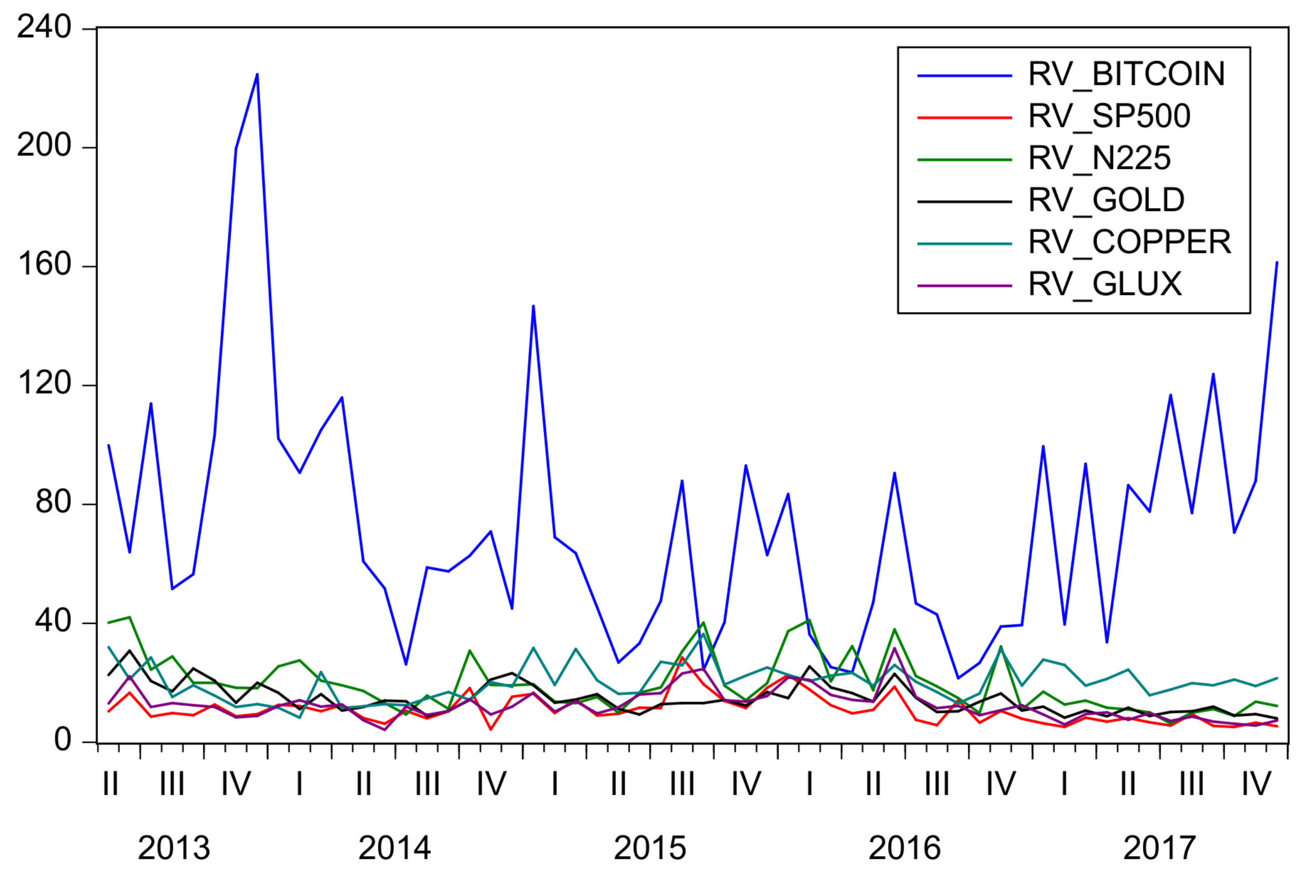
The monthly realized volatilities (RV) are presented in Panel B. Clearly, Bitcoin realized volatility stands out as by far the highest. The average annualized Bitcoin RV is 73% as compared to 11% for the S&P 500. Figure 2 shows the times series of annualized monthly realized volatilities. During the entire sample period Bitcoin realized volatility by far exceeds realized volatility in all other assets. Specifically, the year 2017 was characterized by unusually low volatility in stock markets: in 2017, the Cboe’s volatility index, VIX, fell to the lowest level during the last 23 years and realized volatility in US stock markets was the lowest since the mid-1990s. In sharp contrast, Bitcoin volatility was increasing over almost the entire year.

Panels C and D provide summary statistics for the macro/financial and Bitcoin specific explanatory variables. Prior to the estimation, all explanatory variables are standardized.

Table 2. Contemporaneous correlations between monthly realized volatilities.

	RV-Bitcoin	RV-S&P 500	RV-Nikkei 225	RV-Gold	RV-Copper	RV-Glux
RV-Bitcoin	1.000	−0.074	−0.048	0.059	−0.080	−0.179
RV-S&P 500		1.000	0.636	0.369	0.252	0.818
RV-Nikkei 255			1.000	0.634	0.333	0.743
RV-Gold				1.000	0.220	0.469
RV-Copper					1.000	0.367
RV-Glux						1.000

Notes: The sample covers the 2013M05-2017M12 period. The table reports the contemporaneous correlations between the various realized volatilities.

presents the contemporaneous correlations between the realized volatilities of the different assets. While there is a strong co-movement between the realized volatilities of the S&P 500 and the Nikkei 225 as well as a very strong correlation of both RVs with the realized volatility of the luxury goods index, Bitcoin realized volatility is only weakly correlated with the RV of all other assets. Although the contemporaneous correlations are close to zero, the correlation between $RVo{l}_t^{Bit}$ and $RVo{l}_{t-1}^{SP}$ is −0.1236 and between $RVo{l}_t^{Bit}$ and $RVo{l}_{t-2}^{SP}$ is −0.2623. This suggests that lagged S&P 500 realized volatility may be a useful predictor for future Bitcoin volatility.

In the empirical analysis, we use the explanatory variables in levels. This is justified because the persistence of the explanatory variables is not too strong at the monthly frequency. For example, the first order autocorrelation of the Baltic dry index and trading volume in US dollars is 0.79 and 0.48, respectively. Nevertheless, we also estimated GARCH-MIDAS models using the first difference of the explanatory variables. All our results were robust to this modification.

4. Empirical Results

4.1. Macro and Financial Drivers of Long-Term Bitcoin Volatility

In this section, we analyze the determinants of long-term Bitcoin volatility. In general, once the long-term component is accounted for, the short-term volatility component is well described by a GARCH(1,1) process. As potential drivers of Bitcoin volatility, we consider measures of volatility and risk in the US stock market as well as a measure of global economic activity. These measures have been shown to be important drivers of US stock market volatility in previous studies (see, among others, (Engle et al. 2013; Conrad and Loch 2015; and Conrad and Kleen 2018)). Bouri et al. (2017) found only weak evidence for a relation between US stock market volatility and Bitcoin volatility. However, their analysis was based on daily data and focused on short-term effects. In contrast, the GARCH-MIDAS model allows us to investigate whether US stock market volatility has an effect on long-term Bitcoin volatility. For comparison, we also present how these measures are related to the volatility of the S&P 500, the Nikkei 225 and the volatility of gold and copper.3

As a benchmark model, we estimate a simple GARCH(1,1) for the Bitcoin returns. The parameter estimates are presented in the first line of

Table 3. GARCH-MIDAS for Bitcoin: financial and macroeconomic explanatory variables.

Variable	$\mathit{\mu }$	$\mathit{\alpha }$	$\mathit{\beta }$	m	$\mathit{\theta }$	${\mathit{\omega }}_2$	LLF	AIC	BIC
GARCH(1,1)	$\underset{\left(0.0674\right)}{0.1730{}^{\star \star \star }}$	$\underset{\left(0.0472\right)}{0.1470{}^{\star \star \star }}$	$\underset{\left(0.0507\right)}{0.8560{}^{\star \star \star }}$	$\underset{\left(0.2643\right)}{0.3319{}^{\star \star \star }}$	-	-	$-4738.71$	5.4608	5.4734
RV-S&P 500	$\underset{\left(0.0661\right)}{0.1656{}^{\star \star }}$	$\underset{\left(0.0445\right)}{0.1607{}^{\star \star \star }}$	$\underset{\left(0.0550\right)}{0.8087{}^{\star \star \star }}$	$\underset{\left(0.3775\right)}{2.7211{}^{\star \star \star }}$	$\underset{\left(0.7576\right)}{-2.1114{}^{\star \star \star }}$	$\underset{\left(0.8575\right)}{3.4269{}^{\star \star \star }}$	$-4618.47$	5.4182	5.4374
VIX	$\underset{\left(0.0670\right)}{0.1734{}^{\star \star \star }}$	$\underset{\left(0.0540\right)}{0.1526{}^{\star \star \star }}$	$\underset{\left(0.0691\right)}{0.8236{}^{\star \star \star }}$	$\underset{\left(0.4579\right)}{2.4882{}^{\star \star \star }}$	$\underset{\left(1.2905\right)}{-2.3137{}^{\star }}$	$\underset{\left(1.0696\right)}{3.5195{}^{\star \star \star }}$	$-4627.25$	5.4285	5.4477
RV-Glux	$\underset{\left(0.0648\right)}{0.1813{}^{\star \star \star }}$	$\underset{\left(0.0428\right)}{0.1688{}^{\star \star \star }}$	$\underset{\left(0.0530\right)}{0.7951{}^{\star \star \star }}$	$\underset{\left(0.3701\right)}{2.5390{}^{\star \star \star }}$	$\underset{\left(0.5208\right)}{-1.7776{}^{\star \star \star }}$	$\underset{\left(1.5561\right)}{5.2603{}^{\star \star \star }}$	$-4620.62$	5.4208	5.4399
VRP	$\underset{\left(0.0669\right)}{0.1205{}^{\star }}$	$\underset{\left(0.0390\right)}{0.1939{}^{\star \star \star }}$	$\underset{\left(0.0432\right)}{0.7710{}^{\star \star \star }}$	$\underset{\left(0.5759\right)}{4.8269{}^{\star \star \star }}$	$\underset{\left(1.9478\right)}{6.6860{}^{\star \star \star }}$	$\underset{\left(0.8519\right)}{5.3861{}^{\star \star \star }}$	$-4613.61$	5.4126	5.4317
Baltic	$\underset{\left(0.0650\right)}{0.1946{}^{\star \star \star }}$	$\underset{\left(0.0354\right)}{0.1707{}^{\star \star \star }}$	$\underset{\left(0.0431\right)}{0.7464{}^{\star \star \star }}$	$\underset{\left(0.2503\right)}{3.4942{}^{\star \star \star }}$	$\underset{\left(0.3257\right)}{1.5342{}^{\star \star \star }}$	$\underset{\left(7.8759\right)}{18.3834{}^{\star \star }}$	$-4597.37$	5.3935	5.4127

Notes: The table reports estimation results for the GARCH-MIDAS-X models including 3 MIDAS lag years ($K=36$) of a monthly explanatory variable X. The sample period is 2013M05-2017M12. The conditional variance of the GARCH(1,1) is specified as $h_{i,t}=m+\alpha {\epsilon }_{i-1,t}^2+\beta h_{i-1,t}$. The numbers in parentheses are HAC standard errors. ${}^{\star \star \star }$, ${}^{\star \star }$, ${}^{\star }$ indicate significance at the 1%, 5%, and 10% level. LLF is the value of the maximized log-likelihood function. AIC and BIC are the Akaike and Bayesian information criteria.

. The constant in the mean as well as the two GARCH parameters are highly significant. The sum of the estimates of $\alpha$ and $\beta$ is slightly above one. Therefore, the estimated GARCH model does not satisfy the condition for covariance stationarity. This result is likely to be driven by the extreme swings in Bitcoin volatility and suggests that a two-component model may be more appropriate.4 We also estimated a GJR-GARCH and—in line with Bouri et al. (2017)—found no evidence for asymmetry in the conditional volatility.

The remainder of Table 3 presents the parameter estimates for the GARCH-MIDAS models. For those models, the estimates of $\alpha$ and $\beta$ satisfy the condition for covariance stationarity, i.e., accounting for long-term volatility reduces persistence in the short-term component. First, we use S&P 500 realized volatility as an explanatory variable for long-term Bitcoin volatility. Interestingly, we find that $RVo{l}_t^{SP}$ has a negative and highly significant effect on long-term Bitcoin volatility. Since the estimated weighting scheme puts a weight of 0.09 on the first lag, our parameter estimates imply that a one standard deviation increase in $RVo{l}_t^{SP}$ this month predicts a decline of 17% in long-term Bitcoin volatility next month. The finding that $RVo{l}_t^{SP}$ is negatively related to Bitcoin volatility is in contrast to the usual findings for other markets. For comparison,

Table 4. GARCH-MIDAS for S&P 500.

Variable	$\mathit{\mu }$	$\mathit{\alpha }$	$\mathit{\beta }$	m	$\mathit{\theta }$	${\mathit{\omega }}_2$	LLF	AIC	BIC
RV-S&P 500	$\underset{\left(0.0171\right)}{0.0673{}^{\star \star \star }}$	$\underset{\left(0.0396\right)}{0.1835{}^{\star \star \star }}$	$\underset{\left(0.0552\right)}{0.6818{}^{\star \star \star }}$	$\underset{\left(0.1493\right)}{-0.4549{}^{\star \star \star }}$	$\underset{\left(0.3283\right)}{0.8907{}^{\star \star \star }}$	$\underset{\left(2.6901\right)}{6.9532{}^{\star \star \star }}$	$-1191.81$	2.0371	2.0630
VIX	$\underset{\left(0.0169\right)}{0.0647{}^{\star \star \star }}$	$\underset{\left(0.0381\right)}{0.1717{}^{\star \star \star }}$	$\underset{\left(0.0560\right)}{0.6663{}^{\star \star \star }}$	$\underset{\left(0.1554\right)}{-0.2394}$	$\underset{\left(0.3138\right)}{1.1889{}^{\star \star \star }}$	$\underset{\left(3.3672\right)}{8.7747{}^{\star \star \star }}$	$-1185.90$	2.0270	2.0529
RV-Glux	$\underset{\left(0.0171\right)}{0.0675{}^{\star \star \star }}$	$\underset{\left(0.0418\right)}{0.1897{}^{\star \star \star }}$	$\underset{\left(0.0560\right)}{0.7046{}^{\star \star \star }}$	$\underset{\left(0.1985\right)}{-0.3969{}^{\star \star }}$	$\underset{\left(0.3308\right)}{0.{6072}^{\star }}$	$\underset{\left(2.2863\right)}{9.1559{}^{\star \star \star }}$	$-1194.99$	2.0425	2.0684
VRP	$\underset{\left(0.0169\right)}{0.0625{}^{\star \star \star }}$	$\underset{\left(0.0460\right)}{0.1763{}^{\star \star \star }}$	$\underset{\left(0.0620\right)}{0.7376{}^{\star \star \star }}$	$\underset{\left(0.3327\right)}{-0.3678}$	$\underset{\left(1.0205\right)}{0.8226}$	$\underset{\left(103.8718\right)}{42.9597}$	$-1193.83$	2.0405	2.0664
Baltic	$\underset{\left(0.0174\right)}{0.0662{}^{\star \star \star }}$	$\underset{\left(0.0435\right)}{0.1876{}^{\star \star \star }}$	$\underset{\left(0.0548\right)}{0.7275{}^{\star \star \star }}$	$\underset{\left(0.2314\right)}{-0.7358{}^{\star \star \star }}$	$\underset{\left(0.3218\right)}{-0.3833}$	$\underset{\left(40.4420\right)}{34.5626}$	$-1196.75$	2.0455	2.0714

Notes: See Table 3.

and

Table 5. GARCH-MIDAS for Nikkei 225.

Variable	$\mathit{\mu }$	$\mathit{\alpha }$	$\mathit{\beta }$	m	$\mathit{\theta }$	${\mathit{\omega }}_2$	LLF	AIC	BIC
RV-N225	$\underset{\left(0.0319\right)}{0.0733{}^{\star \star }}$	$\underset{\left(0.0287\right)}{0.1435{}^{\star \star \star }}$	$\underset{\left(0.0407\right)}{0.8118{}^{\star \star \star }}$	$\underset{\left(0.4419\right)}{0.6529}$	$\underset{\left(0.2388\right)}{0.5956{}^{\star \star }}$	$\underset{\left(2.3603\right)}{8.5433{}^{\star \star \star }}$	$-1854.00$	3.2489	3.2753
RV-S&P 500	$\underset{\left(0.0307\right)}{0.0804{}^{\star \star \star }}$	$\underset{\left(0.0270\right)}{0.1256{}^{\star \star \star }}$	$\underset{\left(0.0387\right)}{0.8120{}^{\star \star \star }}$	$\underset{\left(0.2233\right)}{0.9172{}^{\star \star \star }}$	$\underset{\left(1.1214\right)}{2.6059{}^{\star \star }}$	$\underset{\left(1.1835\right)}{2.5956{}^{\star \star }}$	$-1845.16$	3.2335	3.2599
VIX	$\underset{\left(0.0306\right)}{0.0823{}^{\star \star \star }}$	$\underset{\left(0.0266\right)}{0.1194{}^{\star \star \star }}$	$\underset{\left(0.0408\right)}{0.8058{}^{\star \star \star }}$	$\underset{\left(0.2406\right)}{1.2615{}^{\star \star \star }}$	$\underset{\left(0.6460\right)}{2.6210{}^{\star \star \star }}$	$\underset{\left(0.7872\right)}{3.1827{}^{\star \star \star }}$	$-1841.19$	3.2265	3.2530
RV-Glux	$\underset{\left(0.0307\right)}{0.0775{}^{\star \star }}$	$\underset{\left(0.0269\right)}{0.1314{}^{\star \star \star }}$	$\underset{\left(0.0364\right)}{0.8240{}^{\star \star \star }}$	$\underset{\left(0.3341\right)}{1.1043{}^{\star \star \star }}$	$\underset{\left(0.8430\right)}{1.4996{}^{\star }}$	$\underset{\left(4.2353\right)}{4.7827}$	$-1850.32$	3.2425	3.2689
VRP	$\underset{\left(0.0310\right)}{0.0772{}^{\star \star }}$	$\underset{\left(0.0308\right)}{0.1259{}^{\star \star \star }}$	$\underset{\left(0.0379\right)}{0.8494{}^{\star \star \star }}$	$\underset{\left(0.7000\right)}{1.6757{}^{\star \star }}$	$\underset{\left(1.7917\right)}{4.1277{}^{\star \star }}$	$\underset{\left(1.2418\right)}{2.7717{}^{\star \star }}$	$-1851.00$	3.2437	3.2701
Baltic	$\underset{\left(0.0301\right)}{0.0741{}^{\star \star }}$	$\underset{\left(0.0282\right)}{0.1398{}^{\star \star \star }}$	$\underset{\left(0.0356\right)}{0.8522{}^{\star \star \star }}$	$\underset{\left(3.0334\right)}{1.0786}$	$\underset{\left(0.8642\right)}{-1.0354}$	$\underset{\left(5.2701\right)}{10.4773{}^{\star \star }}$	$-1853.51$	3.2480	3.2745

Notes: See Table 3.

present parameters estimates for GARCH-MIDAS models applied to the S&P 500 and the Nikkei 225. As expected, higher levels of $RVo{l}_t^{SP}$ predict increases in S&P 500 long-term volatility as well as increases in the long-term volatility of the Nikkei 225.

Second, we find that the VIX and RV-Glux are negatively related to long-term Bitcoin volatility. Since both measures are positively related to $RVo{l}_t^{SP}$ (see Table 2), this finding is not surprising. Again, Table 4 and Table 5 show that the opposite effect is true for the two stock markets.

Third, Table 3 implies that the VRP has a significantly positive effect on long-term Bitcoin volatility. A high VRP is typically interpreted either as a sign of high aggregate risk aversion (Bekaert et al. (2009)) or high economic uncertainty (Bollerslev et al. (2009)). We observe the same effect for the Nikkei 225 (see Table 5) but no such effect for the S&P 500 (see Table 4).

Fourth, we find a strong positive association between the Baltic dry index and long-term Bitcoin volatility. The finding of a pro-cyclical behavior of Bitcoin volatility is noteworthy, since it contrasts with the counter-cyclical behavior usually observed for financial volatility (see Schwert (1989); or Engle et al. (2013)).

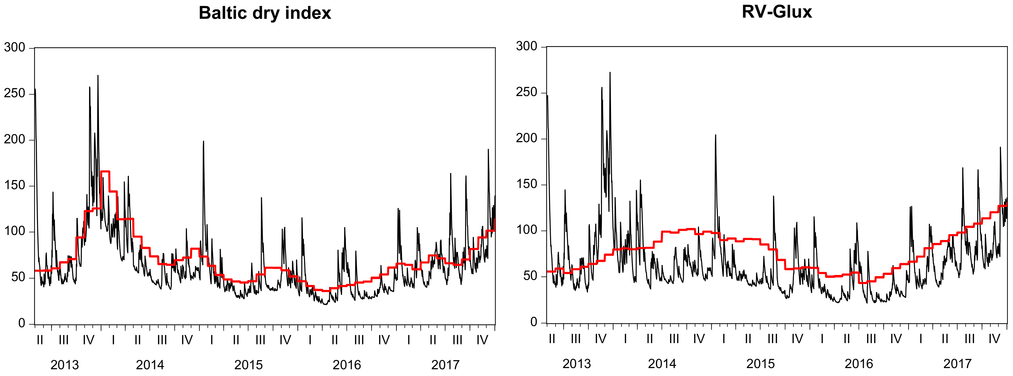
According to the Akaike and Bayesian information criteria, the preferred GARCH-MIDAS model for Bitcoin volatility is based on the Baltic dry index (see Table 3). The left panel of Figure 3 shows the estimated long- and short-term components from this specification. About 65% percent of the variation in the monthly conditional volatility can be explained by movements in long-term volatility. For comparison, the right panel shows the long- and short-term components for the model based on the volatility of the luxury goods index. Clearly, the comparison of graphs confirms that the Baltic dry index has more explanatory power for Bitcoin volatility than RV-Glux.

Finally,

Table 6. GARCH-MIDAS for Gold and Copper.

Variable	$\mathit{\mu }$	$\mathit{\alpha }$	$\mathit{\beta }$	m	$\mathit{\theta }$	${\mathit{\omega }}_2$	LLF	AIC	BIC
Panel A: Gold
RV-S&P 500	$\underset{\left(0.0251\right)}{-0.0079}$	$\underset{\left(0.0085\right)}{0.0217{}^{\star \star }}$	$\underset{\left(0.0169\right)}{0.9653{}^{\star \star \star }}$	$\underset{\left(0.1900\right)}{0.1068}$	$\underset{\left(0.7128\right)}{2.1937{}^{\star \star \star }}$	$\underset{\left(0.6000\right)}{1.9838{}^{\star \star \star }}$	$-1567.17$	2.6732	2.6990
VIX	$\underset{\left(0.0250\right)}{-0.0078}$	$\underset{\left(0.0091\right)}{0.0214{}^{\star \star }}$	$\underset{\left(0.0217\right)}{0.9551{}^{\star \star \star }}$	$\underset{\left(0.1672\right)}{0.3289{}^{\star \star }}$	$\underset{\left(0.4169\right)}{1.9879{}^{\star \star \star }}$	$\underset{\left(0.5787\right)}{2.3936{}^{\star \star \star }}$	$-1564.76$	2.6691	2.6949
RV-Glux	$\underset{\left(0.0251\right)}{-0.0072}$	$\underset{\left(0.0083\right)}{0.0234{}^{\star \star \star }}$	$\underset{\left(0.0136\right)}{0.9689{}^{\star \star \star }}$	$\underset{\left(0.3205\right)}{0.1612}$	$\underset{\left(0.5529\right)}{1.4024{}^{\star \star }}$	$\underset{\left(1.1250\right)}{2.{0356}^{\star }}$	$-1570.45$	2.6788	2.7046
Panel B: Copper
RV-S&P 500	$\underset{\left(0.0349\right)}{-0.0038}$	$\underset{\left(0.0083\right)}{0.0247{}^{\star \star \star }}$	$\underset{\left(0.0113\right)}{0.9640{}^{\star \star \star }}$	$\underset{\left(0.1753\right)}{0.5844{}^{\star \star \star }}$	$\underset{\left(0.0998\right)}{0.{2444}^{\star \star }}$	$\underset{\left(0.0165\right)}{386.9946{}^{\star \star \star }}$	$-1965.14$	3.3494	3.3753
Baltic	$\underset{\left(0.0353\right)}{-0.0086}$	$\underset{\left(0.0119\right)}{0.0262{}^{\star \star }}$	$\underset{\left(0.0384\right)}{0.9369{}^{\star \star \star }}$	$\underset{\left(0.1732\right)}{0.1945}$	$\underset{\left(0.2647\right)}{-0.7006{}^{\star \star \star }}$	$\underset{\left(3.4636\right)}{8.1959{}^{\star \star }}$	$-1965.09$	3.3493	3.3752

Notes: See Table 3.

presents the GARCH-MIDAS estimates for gold and copper. In the table, we include only explanatory variables for which the estimate of $\theta$ is significant. We find that the GARCH persistence parameter, $\beta$, is high for both Gold and Copper across all models. Long-term gold volatility is positively related to realized volatility in the S&P 500, the VIX and realized volatility in the luxury goods index. Interestingly, there is a strongly negative relation between long-term copper volatility and the baltic dry index. Elevated levels of global economic activity go along with high demand for copper and, hence, an increasing copper price and low volatility.

In summary, we find that the behavior of long-term Bitcoin volatility is rather unusual. Unlike volatility in the two stock markets and volatility of gold/copper, Bitcoin volatility decreases in response to higher realized or expected volatility in the US stock market. A potential explanation might be that Bitcoin investors may have lost faith in institutions such as governments and central banks and consider Bitcoin as a safe-haven.5 Furthermore, while stock market volatility and copper volatility behave counter-cyclically, Bitcoin volatility appears to behave strongly pro-cyclically. This is an interesting result that distinguishes Bitcoin from stocks but also from commodities or precious metals. Since Bitcoin neither has an income stream (as compared to stocks) nor an intrinsic value (as compared to commodities), it is often compared to precious metals such as gold. However, our results suggest that the link between Bitcoin volatility and macro/financial variables is very different from the link between those variables and stocks/copper/gold.

4.2. Bitcoin Specific Explanatory Variables

Next, we consider Bitcoin specific explanatory variables. The parameter estimates are presented in

Table 7. GARCH-MIDAS for Bitcoin specific explanatory variables

Variable	$\mathit{\mu }$	$\mathit{\alpha }$	$\mathit{\beta }$	m	$\mathit{\theta }$	${\mathit{\omega }}_2$	LLF	AIC	BIC
Google Trends (all)	$\underset{\left(0.0665\right)}{0.1833{}^{\star \star \star }}$	$\underset{\left(0.0357\right)}{0.1691{}^{\star \star \star }}$	$\underset{\left(0.0450\right)}{0.7863{}^{\star \star \star }}$	$\underset{\left(0.3240\right)}{2.5337{}^{\star \star \star }}$	$\underset{\left(0.0422\right)}{0.0927{}^{\star \star }}$	$\underset{\left(14.9715\right)}{17.7833}$	$-4628.06$	5.4295	5.4486
Google Trends (news)	$\underset{\left(0.0666\right)}{0.1924{}^{\star \star \star }}$	$\underset{\left(0.0367\right)}{0.1870{}^{\star \star \star }}$	$\underset{\left(0.0428\right)}{0.7558{}^{\star \star \star }}$	$\underset{\left(0.3154\right)}{2.4217{}^{\star \star \star }}$	$\underset{\left(0.0207\right)}{0.0622{}^{\star \star \star }}$	$\underset{\left(42.3308\right)}{53.9053}$	$-4614.86$	5.4140	5.4331
US-TV	$\underset{\left(0.0685\right)}{0.1804{}^{\star \star \star }}$	$\underset{\left(0.0365\right)}{0.1598{}^{\star \star \star }}$	$\underset{\left(0.0429\right)}{0.8079{}^{\star \star \star }}$	$\underset{\left(0.3102\right)}{3.4516{}^{\star \star \star }}$	$\underset{\left(0.8046\right)}{-1.9630{}^{\star \star }}$	$\underset{\left(0.6752\right)}{2.1127{}^{\star \star \star }}$	$-4457.43$	5.4234	5.4431
CNY-TV	$\underset{\left(0.0721\right)}{0.1651{}^{\star \star }}$	$\underset{\left(0.0321\right)}{0.1840{}^{\star \star \star }}$	$\underset{\left(0.0386\right)}{0.7731{}^{\star \star \star }}$	$\underset{\left(0.3101\right)}{2.9714{}^{\star \star \star }}$	$\underset{\left(0.2677\right)}{-0.4701{}^{\star }}$	$\underset{\left(3.5819\right)}{11.0465{}^{\star \star \star }}$	$-3387.81$	5.1774	5.2011

Notes: See Table 3.

. As expected, we find that both Google Trend measures (all web searches and monthly news searches) are significantly positively related to Bitcoin volatility. That is, more attention in terms of Google searches predicts higher levels of long-term volatility.6 Finally, we estimate two models that include Bitcoin trading volume in US dollar (US-TV) and Chinese yuan (CNY-TV), respectively. In both cases, we find a significantly negative effect of trading volume. We conjecture that increasing trading volume goes along with higher levels of “trust” or “confidence” in Bitcoin as a payment system and, hence, predicts lower Bitcoin volatility. Recall that Balcilar et al. (2017) analyze the causal relation between trading volume and Bitcoin returns and volatility. They find that volume cannot help predict the volatility of Bitcoin returns. It appears therefore that separating out long-term components is important in finding significant patterns between volatility and trading volume.

5. Conclusions

Cryptocurrency is a relatively unexplored area of research and the fluctuations of Bitcoin prices are still poorly understood. As cryptocurrencies appear to gain interest and legitimacy, particularly with the establishment of derivatives markets, it is important to understand the driving forces behind market movements. We tried to tease out what are the drivers of long-term volatility in Bitcoin. We find that S&P 500 realized volatility has a negative and highly significant effect on long-term Bitcoin volatility and that the S&P 500 volatility risk premium has a significantly positive effect on long-term Bitcoin volatility. Moreover, we find a strong positive association between the Baltic dry index and long-term Bitcoin volatility and report a significantly negative effect of Bitcoin trading volume.

It is worth noting that there are a number of series we considered—such as crime-related statistics—which did not really seem to explain Bitcoin volatility, despite the popular press coverage on the topic. We also experimented with a flight-to-safety indictor suggested in Engle et al. (2012) and found that long-term Bitcoin volatility tends to decrease during flight-to-safety periods. This result squares with our finding of a negative relation between Bitcoin volatility and risks in the US stock market.

Since our findings suggest that Bitcoin volatility forecasts based on the GARCH-MIDAS model are superior to forecasts based on simple GARCH models, our results can be used, for example, to construct improved time-varying portfolio weights when building portfolios of Bitcoins and other assets such as stocks and bonds. Our results may also be useful for the pricing of Bitcoin futures, since they allow us to anticipate changes in Bitcoin volatility at longer horizons. Finally, the GARCH-MIDAS model can be used to simulate Bitcoin volatility based on alternative scenarios for the development of the US stock market or global economic activity. We look forward to sort out these possibilities in future research.

Nevertheless, we would like to emphasize that all our results are based on a relatively short sample period. It will be interesting to see whether our results still hold in longer samples and when the Bitcoin currency has become more mature.

References

- Al-Khazali, Osamah, Bouri Elie, and David Roubaud. 2018. The impact of positive and negative macroeconomic news surprises: Gold versus Bitcoin. Economics Bulletin 38: 373–82. [Google Scholar]
- Balcilar, Mehmet, Elie Bouri, Rangan Gupta, and David Roubaud. 2017. Can volume predict Bitcoin returns and volatility? A quantiles-based approach. Economic Modelling 64: 74–81. [Google Scholar] [CrossRef]
- Baur, Dirk G., Kihoon Hong, and Adrian D. Lee. 2017. Bitcoin: Medium of Exchange or Speculative Assets? Available online: https://ssrn.com/abstract=2561183 (accessed on 25 April 2018). [CrossRef]
- Bekaert, Geert, Eric Engstrom, and Yuhang Xing. 2009. Risk, uncertainty, and asset prices. Journal of Financial Economics 91: 59–82. [Google Scholar] [CrossRef]
- Bollerslev, Tim, George Tauchen, and Hao Zhou. 2009. Expected stock returns and variance risk premia. Review of Financial Studies 22: 4463–92. [Google Scholar] [CrossRef]
- Bouri, Elie, Georges Azzi, and Anne Haubo Dyhrberg. 2017. On the return-volatility relationship in the Bitcoin market around the price crash of 2013. Economics 11: 1–16. [Google Scholar] [CrossRef]
- Chen, Cathy Y. H., Wolfgang Karl Härdle, Ai Jun Hou, and Weining Wang. 2018. Pricing Cryptocurrency Options: The Case of CRIX and Bitcoin. IRTG 1792 Discussion Paper 2018-004. Berlin: Humboldt-Universität zu Berlin. [Google Scholar]
- Cheah, Eng-Tuck, Tapas Mishra, Mamata Parhi, and Zhuang Zhang. 2018. Long memory interdependency and inefficiency in Bitcoin markets. Economics Letters 167: 18–25. [Google Scholar] [CrossRef]
- Conrad, Christian, and Onno Kleen. 2018. Two Are Better Than One: Volatility Forecasting Using Multiplicative Component GARCH Models. Available online: https://ssrn.com/abstract=2752354 (accessed on 15 October 2017).
- Conrad, Christian, and Karin Loch. 2015. Anticipating long-term stock market volatility. Journal of Applied Econometrics 30: 1090–114. [Google Scholar] [CrossRef]
- D’Amuri, Francesco, and Juri Marcucci. 2017. The predictive power of Google searches in forecasting US unemployment. International Journal of Forecasting 33: 801–16. [Google Scholar] [CrossRef]
- Dyhrberg, Anne Haubo. 2016. Bitcoin, gold and the dollar—A GARCH volatility analysis. Finance Research Letters 16: 85–92. [Google Scholar] [CrossRef]
- Engle, Robert, Michael Fleming, Eric Ghysels, and Giang Nguyen. 2012. Liquidity, Volatility, and Flights to Safety in the U.S. Treasury Market: Evidence from a New Class of Dynamic Order Book Models. FRB of New York Staff Report No. 590. Available online: http://0-dx-doi-org.brum.beds.ac.uk/10.2139/ssrn.2195655 (accessed on 9 October 2017).
- Engle, Robert F., Eric Ghysels, and Bumjean Sohn. 2013. Stock market volatility and macroeconomic fundamentals. Review of Economics and Statistics 95: 776–97. [Google Scholar] [CrossRef]
- Fang, Libing, Baizhu Chen, Honghai Yu, and Yichuo Qian. 2018. The importance of global economic policy uncertainty in predicting gold futures market volatility: A GARCH-MIDAS approach. Journal of Futures Markets 38: 413–22. [Google Scholar] [CrossRef]
- Katsiampa, Paraskevi. 2017. Volatility estimation for Bitcoin: A comparison of GARCH models. Economics Letters 158: 3–6. [Google Scholar] [CrossRef]
- Kristoufek, Ladislav. 2015. What are the main drivers of the Bitcoin price? Evidence from Wavelet coherence analysis. PLoS ONE 10: e0123923. [Google Scholar] [CrossRef] [PubMed]
- Khuntia, Sashikanta, and J. K. Pattanayak. 2018. Adaptive market hypothesis and evolving predictability of Bitcoin. Economics Letters 167: 26–28. [Google Scholar] [CrossRef]
- Koutmos, Dimitrios. 2018. Bitcoin returns and transaction activity. Economics Letters 167: 81–85. [Google Scholar] [CrossRef]
- Li, Xin, and Chong Alex Wang. 2017. The technology and economic determinants of cryptocurrency exchange rates: The case of Bitcoin. Decision Support Systems 95: 49–60. [Google Scholar] [CrossRef]
- Polasik, Michal, Anna Iwona Piotrowska, Tomasz Piotr Wisniewski, Radoslaw Kotkowski, and Geoffrey Lightfoot. 2015. Price Fluctuations and the Use of Bitcoin: An Empirical Inquiry. International Journal of Electronic Commerce 20: 9–49. [Google Scholar] [CrossRef]
- Schwert, G. William. 1989. Why does stock market volatility change over time? The Journal of Finance 44: 1115–53. [Google Scholar] [CrossRef]