Market Graph Clustering via QUBO and Digital Annealing

Abstract

We present a novel technique for cardinality-constrained index-tracking, a common task in the financial industry. Our approach is based on market graph models. We model our reference indices as market graphs and express the index-tracking problem as a quadratic K-medoids clustering problem. We take advantage of a purpose-built hardware architecture to circumvent the NP-hard nature of the problem and solve our formulation efficiently. The main contributions of this article are bridging three separate areas of the literature, market graph models, K-medoid clustering and quadratic binary optimization modeling, to formulate the index-tracking problem as a binary quadratic K-medoid graph-clustering problem. Our initial results show we accurately replicate the returns of various market indices, using only a small subset of their constituent assets. Moreover, our binary quadratic formulation allows us to take advantage of recent hardware advances to overcome the NP-hard nature of the problem and obtain solutions faster than with traditional architectures and solvers.

1. Introduction

We present a novel clustering-based formulation for cardinality-constrained index-tracking, a common task in the financial industry. We apply it to data from eight different equity indices from the OR-Library open-source index-tracking data sets and obtain very promising results. We also compare our formulation solved using a purpose-built computational architecture to traditional constrained quadratic formulations solved using a widely available commercial solver, Gurobi.

Our work is an empirical implementation of the K-medoid clustering technique expressed as a quadratic unconstrained binary optimization model (QUBO) and applied to market graphs, for the purpose of obtaining cardinality-contrained index-tracking portfolios. It is inspired by the seminal work of Mantegna (1999), Onnela et al. (2002), Boginski et al. (2003, 2005), Cornuéjols and Tutuncu (2006) and that of Bauckhage et al. (2019). The main contribution in this paper consists of bridging these pieces of complementary but disjoint work, to formulate the index-tracking problem as a QUBO K-medoid clustering of a broader market graph problem. In doing so, we also demonstrate that QUBO reformulations reduce computational times and yield better solutions, because of their suitability to novel purpose-built computer architectures.

Graph clustering is an unsupervised learning task, consisting of assigning common labels to vertices deemed similar. It has found applications in many areas. Chemistry, biology, social networks and finance are a few examples where graph clustering has been applied. However, while there are many competing techniques, the graph clustering problem remains NP-hard, which limits its scope of the application Fortunato (2010); Schaeffer (2007).

QUBO formulations of many mathematical problems have recently gained in interest. This recent spike in interest is, in no small part, due to recent advances and the availability of purpose-built computer architectures that circumvent the NP-hard nature of the problem. Examples of this novel architecture are Fujitsu’s Digital Annealer (DA) and D-Wave’s Quantum Annealer.

Graphs were initially introduced as models of the stock market to gain a robust systemic picture of the market as a whole. In addition, clustering of stock market data is a topic of longstanding interest for both practitioners and academics. Clustering has been used for various purposes, like risk management and portfolio diversification, for example. Index-tracking is another topic of longstanding interest in finance. It consists of building tracking-portfolios whose returns follow a broader index’s returns, but with only a subset of the index constituents. These tracking-portfolios offer the benefit of lower turnover and transaction costs. In the past, some authors in the field have used clustering for the purpose of index-tracking. Their methods identify exemplars of an index and construct tracking-portfolios consisting of only those exemplars.

We formulate the index-tracking problem as a QUBO graph-clustering problem. Our formulation restricts the number of assets while identifying the most representative exemplars of an index. Our thesis is that a portfolio consisting of the most representative set of exemplars will minimize tracking-error. Initial results are very encouraging. Our tests show we accurately replicate the returns of broad market indices, using only a small subset of their constituent assets. Moreover, our QUBO formulation allows us to take advantage of recent hardware advances to overcome the NP-hard nature of the clustering problem. Using these novel architectures we obtain better solutions within small fractions of the time required to solve equivalent problems formulated in traditional constrained form and solved on traditional hardware. Our initial results certainly offer hope and set the stage for larger-scale problems, in finance and beyond.

The remainder of this article is organized as follows. We begin with an overview of three disjoint but complementary areas of the literature, market graph modeling, index-tracking and clustering. We then describe our K-medoid based formulation for clustering the market graph and the novel purpose-built computational tools we use to solve it. Finally, we apply our technique to a set of equity indices.

2. Previous Work

Our work lies at the intersection of graph models of the stock markets, clustering, combinatorial optimization (QUBO) and (stock market) index-tracking. In this section, we briefly review these areas of research. Our goal is not to provide the reader with a detailed review of state of the art in these very broad fields, but rather to focus specifically on their relevance to the work in this article, in order to put it in proper context.

2.1. Market Graph

The use of graphs as models of the stock market was initially introduced in the literature by Mantegna (1999) and Onnela et al. (2002). These authors introduced graph-based modeling because of its ability to capture hierarchical structures in markets and its robustness to market movements. Other authors have also highlighted the advantage of using market graphs in lieu of covariance matrices, due to their robustness to noise and estimation error Tola et al. (2008). The extensive work of Boginski et al. (2003, 2004a, 2004b, 2005, 2006) was also pivotal in establishing graphs as a modeling tool for financial markets. The common thread connecting all these authors’ work is the modeling of stocks as vertices in a weighted graph, where edge weights are proportional to their returns correlations.

Other authors have also followed up on and expanded this work by studying market graph dynamics over time Arratia and Cabaña (2011); Kocheturov et al. (2014) and examined methods for building the graph Bautin et al. (2013); Kalyagin et al. (2018); Koldanov et al. (2013). In fact, to this day, the topic of graphs as a model for equity markets remains a subject of discussion in the literature Abrams (2016); Marti et al. (2019).

2.2. Cardinality-Constrained Index-Tracking

Typically, portfolio optimization consists of finding a combination of financial assets that maximize expected returns, subject to some return volatility constraints, through the use of mathematical (quadratic) programming. This mathematically formal portfolio construction technique was initially introduced by Markowitz (1952), in the 1950s. Unfortunately, this approach is not robust to errors in returns forecasting or covariance estimation Michaud (2014). Additionally, it has been documented that equally-weighted portfolios often outperform portfolios with more complicated weighting schemes DeMiguel et al. (2007) and that index funds offer the best risk-return trade-off Cornuéjols and Tutuncu (2006).

In the presence of estimation error and the problem of obtaining reliable return forecasts, some authors suggested that the optimal investment strategy consists of simply following broad market indices Cornuéjols and Tutuncu (2006); Treynor and Black (1973). In line with the goal of designing portfolios that follow an index’s returns, the index-tracking problem consists of minimizing a portfolio’s return deviations from those of a reference market index.

Cardinality-constrained index-tracking is the process of tracking an index with a subset of its constituents. Portfolio managers opt for this approach because it reduces turnover and transaction costs and allows for more liquid portfolios. For example, in 2008, a mixed integer linear programming approach was applied to a large array of equity market indices Beasley (1990); Canakgoz and Beasley (2009). More recently, some authors have formulated the cardinality-constrained index-tracking problem in QUBO form Corp (2018). These authors’ work differs from our formulation. They seek to minimize tracking-error using a traditional portfolio risk metrics and do not make use of the more robust market graphs. Nevertheless, these authors set the stage for the work presented in this article. It should also be noted that finding the subset of at most k assets whose returns best track a given index’s was shown to be an NP-hard problem Mutunge and Haugland (2018).

2.3. Clustering for Index-Tracking

Clustering is the process of grouping similar (dissimilar) observations. Graph clustering is the process of assigning common labels to vertices deemed (dis)similar. It has a long history in the literature. A thorough review of the graph clustering literature is beyond the scope of this article. For a very comprehensive view of the field, we refer the reader to the foundational work of Schaeffer (2007), Fortunato (2010) and the recent contribution by Fortunato and Hric (2016). We do, however, echo these authors and emphasize the fact that graph clustering is an NP-hard problem.

The link between clustering and portfolio construction is of particular relevance to the work in our article Boginski et al. (2014); Chen and Kwon (2012); Cornuéjols and Tutuncu (2006); Kalyagin et al. (2014); Puerto et al. (2020); Wu et al. (2017). Although not focused specifically on graph clustering, Cornuéjols and Tutuncu (2006) presented a K-medoid formulation for index-tracking. These authors used a K-medoid technique Hastie et al. (2009) to find k representative stocks (exemplars) that compose a portfolio that replicates the returns of a broader index. Unfortunately, their formulation leads to an NP-hard problem Nascimento et al. (2012).

More recently, Bauckhage et al. (2019) reformulated the K-medoids problem in QUBO form Glover et al. (2018); Lucas (2014). They formulated a QUBO model that selects the most central points that are also the most mutually distant, in order to obtain a good summary of the underlying data set. To obtain an unconstrained model, these authors applied a penalty function to relax their model’s constraints. In the end, they offered a model that can be implemented on purpose-built hardware designed to circumvent the NP-hardness of such reformulated combinatorial optimization problems. Indeed, this reformulation allows us to take advantage of recent hardware advances specifically designed for QUBO formulations Aramon et al. (2019); Matsubara et al. (2020). In the same vein, to circumvent the NP-hardness of a problem closely related to graph clustering, the maximum weighted independent set of the graph, and produce a well diversified portfolio of Dow Jones stocks, Marzec (2013) implemented the work of Boginski et al. (2005) using the D-Wave adiabatic quantum computation system.

In recent years, others have also examined portfolio construction via graph models. For example, Kalyagin et al. (2014) compared the Markowitz portfolio theory Markowitz (1952) to the market graph Boginski et al. (2005). They reduced the pool of assets using historical returns, variance, and Sharpe ratio to build a market graph. Then, they examined the efficient frontiers of the maximal independent set and the maximal clique of a market graph.

3. Methods

We begin by representing eight different equity indices as market graphs. Each index is modeled as a weighted complete graph. The constituent stocks are represented by a vertex and edge weights are a function of each asset-pair’s returns correlations. We then apply a K-medoid index-tracking technique to find k exemplars that will form our tracking-portfolio. To take advantage of a fast purpose-built computer architecture, the Fujitsu Digital Annealer (DA), we express the K-medoid problem as a QUBO problem. Finally, the tracking-portfolios are developed following the weight allocation method described in Cornuéjols and Tutuncu (2006). In the end, we create a tracking-portfolio for each index in our study.

3.1. Market Graph

We represent each index as a complete weighted graph, where edge weights represent the association between stocks ‘i’ and ‘j’. These weights are defined using the Pearson correlation coefficient ($\rho$) Walpole (2011) of the log daily returns of each asset pair,

$$d_{ij}=\sqrt{\frac{1}{2}\left(1-{\rho }_{ij}\right)}.$$

In modeling the market in this way, our investment universe is modeled as a set of complete weighted graphs (one for each index), with no self-loops (since ${\rho }_{ii}=1$). Also, our transformation from returns correlation $\left({\rho }_{ij}\right)$ to distance $\left(d_{ij}\right)$ provides a smoother and more robust measure of returns (dis)similarity and market fluctuations.

To be consistent with the QUBO formulation of Bauckhage et al. (2019), we convert our adjacency (distance) matrix into a more robust matrix $\Delta =\left[{\delta }_{ij}\right]$, with the elements ${\delta }_{ij}=1-exp(-\frac{1}{2}\times d_{ij})$. We note that this formulation requires all-pairs distances ($d_{ij}$) be known, which is why we use a complete graph representation.

3.2. Data Sets

We use the freely available data sets of Beasley’s OR-Library Beasley (1990). This curated data set, which was updated in 2007, contains weekly data for a portion of the constituents of eight major equity indices. Some data cleaning was conducted on these indices, by its curators. As a result, the published data sets only contain a subset of the constituent securities of the indices. The indices and the number of constituents included in the final published data sets are shown in

Table 1. Indices and Number of Constituents in Sample.

Index	Num Stocks
DAX 100	84
FTSE 100	88
Hang Seng	30
Nikkei 225	224
Russell 2000	1317
Russell 3000	2150
Standard and Poors 100	97
Standard and Poors 500	456

.

The data covers period from March 1992 to September 1997. For each asset, there are a total of 290 observations. We use the first 145 to construct our market graphs and the other half of the data to measure the tracking performance.

3.3. QUBO Model

We follow the method developed by Bauckhage et al. (2019). Our K-medoids formulation makes use of a tradeoff parameter to find an optimal combination of dispersed and central stocks, on the market graph. These stocks are selected because their fluctuations are representative of those of their respective index (market graph). For this reason, these stocks are also referred to as “exemplars”.

In the formulations that follow, $z_i=1$ if vertex i is selected as an exemplar and $z_i=0$ otherwise. The vector $\mathbf{1}$ is a vector of ones of appropriate dimension. The matrix $\Delta$ is an $(n\times n)$ matrix containing the distances separating all stock-stock pairs denoted $d_{ij}$.

$$\begin{array}{ccc}\hfill z& =& [z_1{z}_2\dots z_n],\forall z_i\in \{0,1\}\hfill \\ \hfill \mathbf{1}& =& [11\dots 1]\in {\mathbb{R}}^n\hfill \\ \hfill \Delta & =& \left[{\delta }_{ij}\right]\hfill \end{array}$$

Model (1) seeks to find k nodes that are considered the most central within the graph,

$$\begin{array}{cccc}\hfill & \underset{z}{min}\hfill & \hfill & z^T\Delta \mathbf{1}\hfill \\ \hfill & \mathrm{s}.\mathrm{t}\hfill & \hfill & z^T\mathbf{1}=k\hfill \\ \hfill & \hfill & & z_i\in \{0,1\},\forall i\in V.\hfill \end{array}$$

(1)

Meanwhile, model (2) seeks to find k nodes that are considered most dispersed within the graph,

$$\begin{array}{cccc}\hfill & \underset{z}{max}\hfill & \hfill & \frac{1}{2}{z}^T\Delta z\hfill \\ \hfill & \mathrm{s}.\mathrm{t}\hfill & \hfill & z^T\mathbf{1}=k\hfill \\ \hfill & \hfill & & z_i\in \{0,1\},\forall i\in V.\hfill \end{array}$$

(2)

We then apply the $\alpha -\beta$ tradeoff parameters to weigh the contributions of Model (1) and Model (2). Our ultimate goal is to find portfolios consisting of k exemplars that best replicate the returns of each index in our study. To achieve this goal, we proceed as follows:

$$\begin{array}{cccc}\hfill & \underset{z}{min}\hfill & \hfill & \left\{f=\beta z^T\Delta \mathbf{1}-\alpha \frac{1}{2}{z}^T\Delta z\right\}\hfill \\ \hfill & \mathrm{s}.\mathrm{t}\hfill & \hfill & z^T\mathbf{1}=k\hfill \\ \hfill & \hfill & & z_i\in \{0,1\},\forall i\in V.\hfill \end{array}$$

(3)

By applying a quadratic penalty, we obtain a QUBO K-medoids formulation:

$$\begin{array}{cccc}\hfill & \underset{z}{min}\hfill & \hfill & \left\{f_o=\beta z^T\Delta \mathbf{1}-\alpha \frac{1}{2}{z}^T\Delta z+\gamma {\left(z^T\mathbf{1}-k\right)}^2\right\}\hfill \\ \hfill & \hfill & & z_i\in \{0,1\},\forall i\in V.\hfill \end{array}$$

(4)

The model shown in Equation (4) defines the optimization problem where the decision variables, $z_i$, take on the value $z_i=1$ if node i is an exemplar node and 0 otherwise. The parameter $\alpha$ is the weight assigned to the total contribution of the max-sum dispersion model. The parameter $\beta$ is the weight of the total contribution from the centrality of exemplars. Finally, the parameter $\gamma$ is the penalty coefficient that enforces feasibility. It pushes the solution $z^{*}$ towards k non-zero entries.

3.4. Parameters

We follow the example of Bauckhage et al. (2019) and set $\alpha =\frac{1}{k}$ and $\beta =\frac{1}{n}$, as suggested. However, the convergence of the QUBO model and the feasibility of the solution both depend on the penalty coefficient $\gamma$. The process for determining an adequate value of $\gamma$ is a bit more complicated and involves trial and error.

To make these trials, which we conduct over a range of values, more efficient, we begin with a reasonable guess. Here, we follow the advice of Glover et al. (2018), who suggest exploring a range of reasonable values. To obtain our initial guess, we use a naïve average-case approximation for $\gamma$, which we label $\tilde{\gamma }$. For the purpose of this approximation, we use an average distance matrix $\overline{\Delta }=\left[{\overline{\delta }}_{ij}\right]$, instead of the matrix $\Delta$. The elements of this matrix are defined as:

$${\overline{\delta }}_{ij}=\left\{\begin{array}{cc}\frac{1}{n(n-1)}\sum _{i=1}^n\sum _{j=1}^n{\delta }_{ij},\hfill & \mathrm{if}i\ne j(\mathrm{recall}{\delta }_{ii}=0)\hfill \\ 0,\hfill & \mathrm{otherwise}.\hfill \end{array}\right.$$

We also note the parameter $\gamma$ multiplies squared deviations from feasibility and the unit penalty is observed when we have ($k\pm 1$) non-zero entries. However, the value of the un-penalized objective function is higher when we have ($k+1$) non-zero entries. Since optimization routines will naturally favor solutions with fewer non-zero elements, the ($k+1$) case is uninteresting. For this reason, we define our initial guess for $\gamma$ as the difference between the naïvely approximated un-penalized objective functions, $f\left(\right)$, with solutions containing k and $(k-1)$ exemplars. To do so, we define the following variables.

• z is a solution containing $(k-1)$ exemplars. It is infeasible.
• $z^{*}$ is a solution containing k exemplars. It is feasible.
• Both these vectors are in ${\mathbb{R}}^n$.
• Therefore, we have the equality ${\sum }_i{z}_i^{*}=\left({\sum }_i{z}_i\right)+1=k$.

Our initial guess for $\gamma$, which we call $\tilde{\gamma }$, is defined as:

$$\begin{array}{ccc}\hfill f\left(z^{*}\right)& \approx & \left(\beta \sum _{i=1}^n{z}_i^{*}\sum _{j=1}^n\overline{\delta }\right)-\left(\frac{\alpha }{2}\sum _{i=1}^n\sum _{j=1}^n{z}_i^{*}{z}_j^{*}\overline{\delta }\right)\hfill \\ & \approx & \beta kn\overline{\delta }-\frac{\alpha }{2}k(k-1)\overline{\delta },\hfill \\ \hfill f\left(z\right)& \approx & \left(\beta \sum _{i=1}^n{z}_i\sum _{j=1}^n\overline{\delta }\right)-\left(\frac{\alpha }{2}\sum _{i=1}^n\sum _{j=1}^n{z}_i{z}_j\overline{\delta }\right)\hfill \\ & \approx & \beta (k-1)n\overline{\delta }-\frac{\alpha }{2}(k-1)(k-2)\overline{\delta },\hfill \\ \hfill \tilde{\gamma }& =& \left(\beta kn\overline{\delta }-\frac{\alpha }{2}k(k-1)\overline{\delta }\right)-\left(\beta (k-1)n\overline{\delta }-\frac{\alpha }{2}(k-1)(k-2)\overline{\delta }\right)\hfill \\ & =& \frac{\overline{\delta }}{k}(\mathrm{Substituting}\mathrm{for}\alpha ,\beta ).\hfill \end{array}$$

(5)

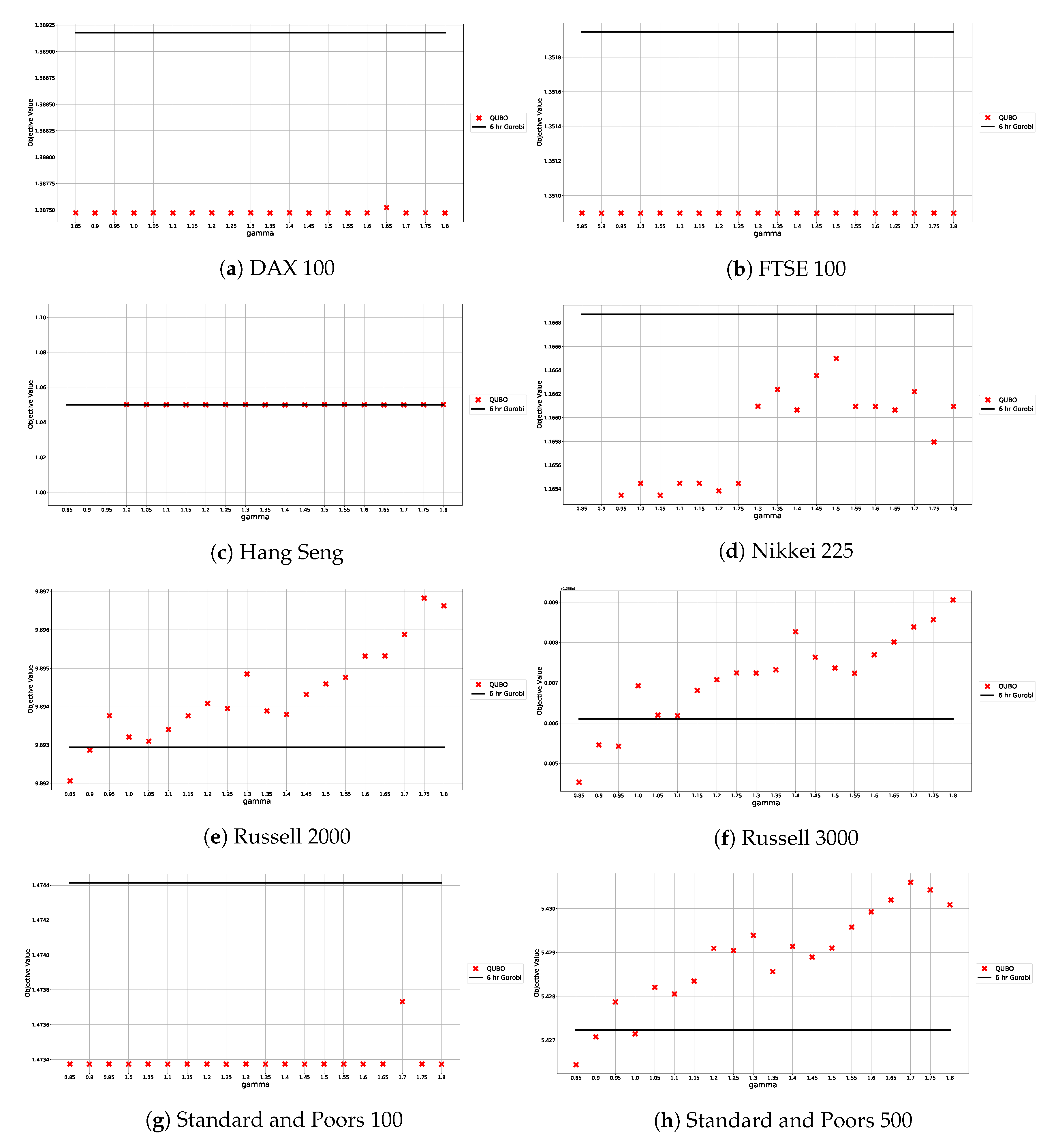
We then use this initial guess as a starting point to perform 20 numerical tests with varying $\gamma$ coefficients, for each data set in our study. For each graph, we examine the impact of the penalty parameter on the objective function by testing values in the range $\gamma \in [0.85\times \tilde{\gamma },1.8\times \tilde{\gamma }]$. Results are shown in Figure 1. The actual values of our initial guesses $\tilde{\gamma }$ are shown in

Table 2. Initial Guesses $\tilde{\gamma }$.

Index	$\tilde{\mathit{\gamma }}$
DAX 100	0.026
FTSE 100	0.025
Hang Seng	0.019
Nikkei 225	0.022
Russell 2000	0.004
Russell 3000	0.003
Standard and Poors 100	0.027
Standard and Poors 500	0.007

. Since distance matrices are specific to each index (market graph), we have an initial guess for each.

3.5. The Fujitsu DA: Purpose-Built Architecture

To circumvent the NP-hard nature of the clustering problem, we use a purpose built computer architecture, the Fujitsu Digital Annealer (DA). The DA provides fast computation and is designed specifically for combinatorial optimization problems expressed in QUBO form Aramon et al. (2019); Matsubara et al. (2020).

With the exception of the benchmark tests described in Section 4.3, all of our computations for the minimization of the model described in Section 3.3 were done using this architecture 1. For benchmarking, we compare our computational results to those obtained using the Gurobi solver.

3.6. Asset Weights

Once the k exemplar assets have been identified, an allocation weight for each asset is determined following the method described by Cornuéjols and Tutuncu (2006). We begin by assigning every stock to a cluster formed by grouping nodes around their nearest exemplar node. Then, each exemplar node i is weighted using the following equation:

$$w_i=\frac{{\sum }_j{P}_j{x}_{ij}}{{\sum }_i{\sum }_j{P}_j{x}_{ij}},\mathrm{where}{P}_j\mathrm{is}\mathrm{the}\mathrm{market}\mathrm{value}\mathrm{of}\sec \mathrm{urity}j,$$

with

$$x_{ij}=\left\{\begin{array}{c}1,\mathrm{if}\mathrm{node}i\mathrm{is}\mathrm{the}\mathrm{closest}\mathrm{exemplar}\mathrm{node}\mathrm{to}\mathrm{node}j\hfill \\ 0,\mathrm{otherwise}.\hfill \end{array}\right.$$

(Naturally, ${\sum }_i{w}_i=1$.)

4. Numerical Experiments

We use our K-medoid technique to construct eight index-tracking-portfolios, one for each index in our study (see Table 1). For each index, we use the first 145 observations to compute stock-to-stock distances, build a market graph and corresponding distance matrix $\Delta$. We then optimize the QUBO model to obtain the k exemplars that form each of our tracking-portfolios.

To assess tracking accuracy, we use tracking-error, as per industry practice. For each index, we compute the differences between the daily log returns of our tracking-portfolio and it respective benchmark’s. We calculate the standard deviation of the differences to obtain the annual tracking-error.

For benchmarking purposes, we also examine the computational performance of our QUBO model solved on purpose-built hardware. We compare it to an equivalent 0–1 quadratic constrained program solved using a commercial solver, Gurobi, running on conventional hardware. While performing these comparisons, we also examine the effect varying $\gamma$ has on the QUBO solutions.

4.1. Test Data

As mentioned earlier, we use Beasley’s OR-Library data Beasley (1990) to build our market graphs and assess the performance of our tracking-portfolios. We use the same cardinality constraints as Canakgoz and Beasley (2009). The number of assets in each of the tracking-portfolios is shown in

Table 3. Indices and Number of Constituents in Tracking-Portfolios.

Index	Cardinality Constraint $\left(\mathit{k}\right)$
DAX 100	10
FTSE 100	10
Hang Seng	10
Nikkei 225	10
Russell 2000	90
Russell 3000	70
Standard and Poors 100	10
Standard and Poors 500	40

.

As also mentioned previously, these data sets contain 290 weekly observations. We use the first 145 observations to build our graphs and tracking-portfolios and the remaining 145 to assess the tracking performance.

4.2. Index-Tracking Performance

Tracking-error is the standard deviation of the difference in returns between each index-portfolio–tracking-portfolio pair of observations, at a given time point (weekly in this case). We denote log weekly returns for the reference index and the tracking-portfolio as $r_{\mathrm{index}}$ and $r_{\mathrm{port}}$, respectively. We denote, tracking-error as $ϵ$ and compute it as

$$\begin{array}{ccc}\hfill d& =& r_{\mathrm{index}}-r_{\mathrm{port}}\hfill \\ \hfill ϵ& =& \sqrt{Var\left[d\right]}.\hfill \end{array}$$

We report the tracking-error of each of our tracking-portfolios, in

Table 4. Tracking-Error.

Index	Tracking-Error
DAX 100	0.0118
FTSE 100	0.0096
Hang Seng	0.0089
Nikkei I225	0.0223
Russell 2000	0.0187
Russell 3000	0.0123
Standard and Poors 100	0.0097
Standard and Poors 500	0.0137

.

Our empirical results show that our tracking-portfolios yield returns that closely reflect those of their reference index. For all our index-tracking portfolios, we note that tracking-error remains in the order of two percent, or less. This performance is very typical of tracking-portfolios. In fact, our tracking-errors are of the same order of magnitude as those obtained by Wu et al. (2017) on a different data set.

4.3. Computation Times, Objective Function and $\gamma$

In order to examine the computational performance of our QUBO reformulation and purpose-built architecture, we solve the equivalent constrained 0–1 quadratic program using Gurobi version 7.5.2. We run Gurobi on a 64-bit Supermicro X10DAi with an Intel Xeon CPU E5-2697 v4 @2.3GHz with 18 cores and 256GB of RAM. We set an upper run time limit for Gurobi of 10,700 s (approx 3 h), an amount approximately 20 times the average DA run time. Here again, we repeat these experiments for each index in our study.

In

Table 5. Run Times and Objective Function.

Index	DA Run Time	DA Obj Fn	Gi Run Time	Gi Obj Fn
DAX100	520	1.388	10,712	1.389
FTSE100	522	1.351	10,712	1.352
Hang Seng	520	1.050	70	1.050
Nikkei 225	522	1.165	10,701	1.167
Russell 2000	532	9.892	10,700	9.893
Russell 3000	589	12.585	10,703	12.586
SP 100	522	1.473	10,700	1.474
SP 500	523	5.426	10715	5.427

, we note that Gurobi very quickly converges to a sub-optimal solution, in the case of the Hang Seng, the easiest problem instance in our tests. That problem instance consists of obtaining a set of 10 exemplars from a set of 30 stocks. The DA returns an equivalent solution, although after a much longer computation. In contrast, Gurobi fails to converge, in all other instances. Meanwhile, the DA returns better solutions in less than nine minutes, in all other experiments. Details of these experiments are shown in Table 5.

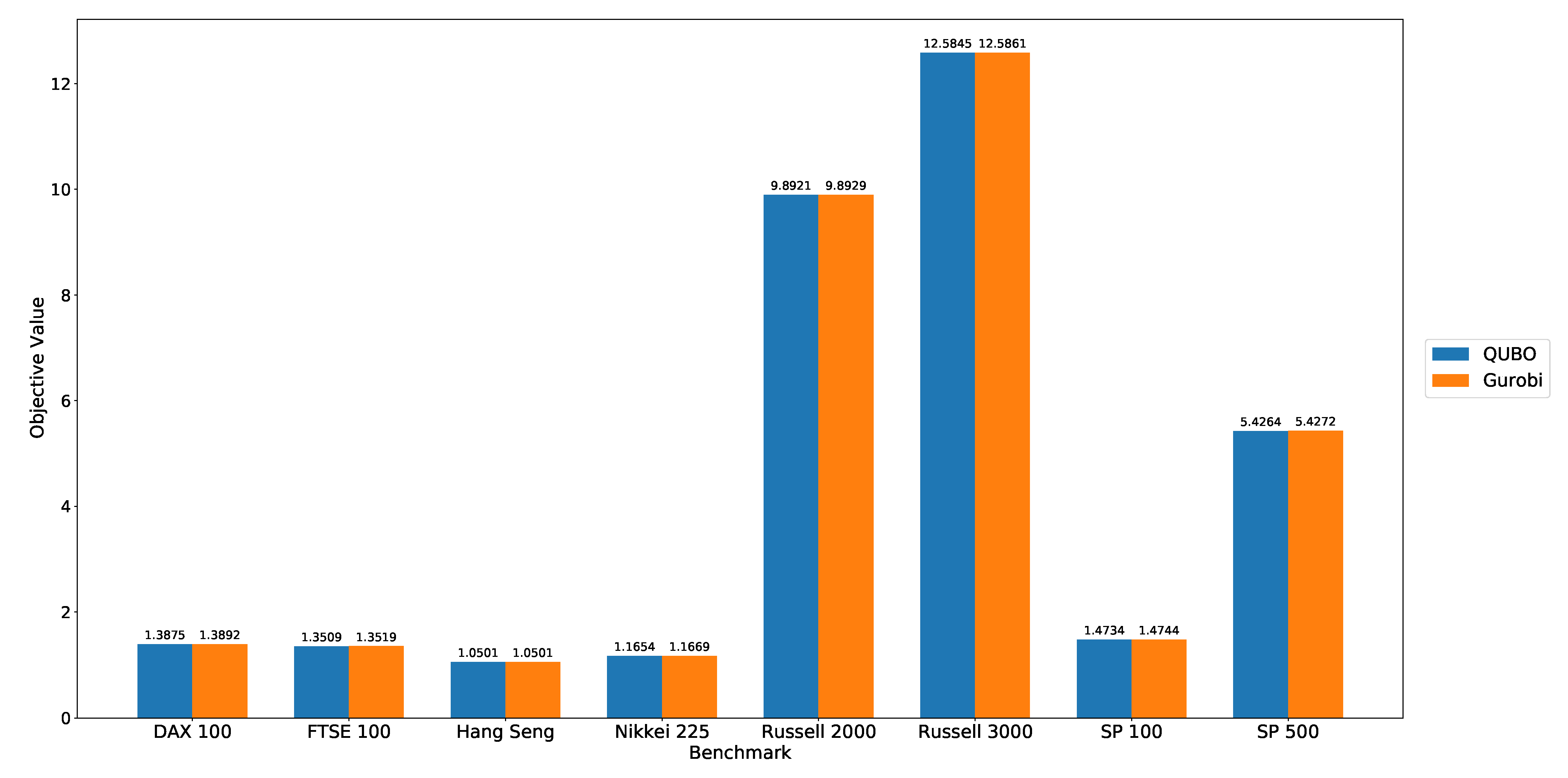
The solutions returned by the DA are better (lower) than those yielded by Gurobi, in seven out of eight experiments. These results are shown in Figure 2. It should be noted, however, that neither the DA nor Gurobi solutions are optimal. Through a Monte-Carlo simulation of randomly generated feasible solutions, we were able to observe marginally better solutions.

To examine the sensitivity of the QUBO objective function to the penalty cofficient $\gamma$, we test a range of values and record the resulting objective function values obtained. As described in Section 3.4, we explore a range of $\gamma$ values in the interval $[0.85\times \tilde{\gamma },1.8\times \tilde{\gamma }]$. Experimental results are shown in Figure 1, where objective function values for varying $\gamma$ coefficients are also compared to those obtained by solving the constrained program using Gurobi (solid line).

While variations in $\gamma$ do affect the objective function, this effect remains very small. Nevertheless, for the purpose of portfolio construction we set $\gamma$ to the value that minimizes the objective function, for each index. (It also yields a better objective value than what was attained with Gurobi.) Actual values for each index are shown in

Table 6. Penalty Coefficients $\gamma$ that Minimize the Objective Function.

Index	Best $\mathit{\gamma }$
DAX 100	0.022
FTSE 100	0.021
Hang Seng	0.019
Nikkei 225	0.021
Russell 2000	0.003
Russell 3000	0.003
Standard and Poors 100	0.023
Standard and Poors 500	0.006

.

5. Conclusions and Discussion

In this article, we have joined three complementary areas of the mathematical sciences, to efficiently solve a concrete commercial problem, cardinality-constrained equity index-tracking. Our work combines the complementary but disjoint areas of graph models of equity markets, QUBO reformulations of combinatorial optimization problems and clustering.

Our results show that a QUBO formulation of the K-medoid problem can be successfully used to replicate broad market indices, using just a small portion of their constituent assets. In all eight of our experiments, we track our target indices with a tracking-error in the order of two percent, or less. These results show significant commercial promise, since they demonstrate that large indices can be replicated with a small portion of their constituents. By applying our technique, portfolio managers can reduce transaction costs and turnover significantly.

Naturally, our conclusions are limited to the data sets and time period in our study. Broader tests are still required to determine the commercial viability of our technique.

On the mathematical and computational side, our results illustrate the usefulness of QUBO reformulations and purpose-built architecture for solving them. Through our reformulation, we obtain better results faster than with a traditional constrained quadratic programming formulation and solver. This QUBO advantage is likely to be even greater on larger-scale problems. We can also realistically expect the QUBO advantage to hold even more strongly in large-scale optimization problems in other areas, especially those dealing with “big data”.

Our future work will begin with tests of the techniques described in this article on other data sets, especially data sets covering a wider array of time periods. We will also explore alternate techniques for building the market graph and determining the optimal cardinality of the tracking subset. From a mathematical and computational point of view, we also intend to investigate other applications, alternate problem formulations and larger scale optimization.

References

- Abrams, Joshua. 2016. Analysis of equity markets: A graph theory approach. Society for Industrial and Applied Mathematics. [Google Scholar] [CrossRef]
- Aramon, Maliheh, Gili Rosenberg, Elisabetta Valiante, Toshiyuki Miyazawa, Hirotaka Tamura, and Helmut G. Katzgraber. 2019. Physics-Inspired Optimization for Quadratic Unconstrained Problems Using a Digital Annealer. Frontiers in Physics 7. [Google Scholar] [CrossRef] [Green Version]
- Arratia, Argimiro, and Alejandra Cabaña. 2011. A graphical tool for describing the temporal evolution of clusters in financial stock markets. Computational Economics 41. [Google Scholar] [CrossRef] [Green Version]
- Bauckhage, Christian, Nico Piatkowski, Rafet Sifa, Dirk Hecker, and Stefan Wrobel. 2019. A QUBO formulation of the k-medoids problem. Paper present at Conference on “Lernen, Wissen, Daten, Analysen”, Berlin, Germany, September 30–October 2; 2454 vols.. Edited by R. Jäschke and M. Weidlich. Berlin: CEUR Workshop Proceedings, pp. 54–63. [Google Scholar]
- Bautin, Grigory, Valery A. Kalyagin, Alexander Koldanov, Petr Koldanov, and Panos M. Pardalos. 2013. Simple measure of similarity for the market graph construction. Computational Management Science 10: 6. [Google Scholar] [CrossRef]
- Beasley, John. 1990. Or-library: Distributing test problems by electronic mail. Journal of the Operational Research Society 41: 1069–72. [Google Scholar] [CrossRef]
- Boginski, Vladimir, Sergiy Butenko, and Panos M. Pardalos. 2003. On structural properties of the market graph. Innovations in Financial and Economic Networks 48: 29–35. [Google Scholar]
- Boginski, Vladimir, Sergiy Butenko, and Panos M. Pardalos. 2004a. Network-Based Techniques In The Analysis Of The Stock Market. In Supply Chain and Finance. Edited by P. M. Pardalos, A. Migdalas and G. Baourakis. World Scientific Book Chapters. Singapore: World Scientific Publishing Co. Pte. Ltd., chp. 1. pp. 1–14. [Google Scholar]
- Boginski, Vladimir, Sergiy Butenko, and Panos M. Pardalos. 2004b. Network models of massive datasets. Computer Science and Information Systems 1: 75–89. [Google Scholar] [CrossRef]
- Boginski, Vladimir, Sergiy Butenko, and Panos M. Pardalos. 2005. Statistical analysis of financial networks. Computational Statistics & Data Analysis 48: 431–43. [Google Scholar] [CrossRef]
- Boginski, Vladimir, Sergiy Butenko, and Panos M. Pardalos. 2006. Mining market data: A network approach. Computers & Operations Research 33: 3171–84. [Google Scholar] [CrossRef]
- Boginski, Vladimir, Sergiy Butenko, Oleg Shirokikh, Svyatoslav Trukhanov, and Jaime G. Lafuente. 2014. A network-based data mining approach to portfolio selection via weighted clique relaxations. Annals of Operations Research 216: 23–34. [Google Scholar] [CrossRef]
- Canakgoz, Nilgun A., and John E. Beasley. 2009. Mixed-integer programming approaches for index tracking and enhanced indexation. European Journal of Operational Research 196: 384–99. [Google Scholar] [CrossRef]
- Chen, Chen, and Roy H. Kwon. 2012. Robust portfolio selection for index tracking. Computers & Operations Research 39: 829–37. [Google Scholar] [CrossRef]
- Cornuéjols, Gérard, and Reha Tutuncu. 2006. Optimization Methods in Finance. Mathematics, Finance and Risk. Cambridge: Cambridge University Press. [Google Scholar]
- QC Ware Corp. 2018. A Quadratic Unconstrained Binary Optimization Problem Formulation for Single-Period Index Tracking with Cardinality Constraints. Technical Report. Palo Alto: QC Ware. [Google Scholar]
- DeMiguel, Victor, Lorenzo Garlappi, and Raman Uppal. 2007. Optimal versus naive diversification: How inefficient is the 1/NPortfolio strategy? Review of Financial Studies 22: 1915–53. [Google Scholar] [CrossRef] [Green Version]
- Fortunato, Santo. 2010. Community detection in graphs. Physics Reports 486: 75–174. [Google Scholar] [CrossRef] [Green Version]
- Fortunato, Santo, and Darko Hric. 2016. Community detection in networks: A user guide. arXiv e-prints arXiv:1608.00163. [Google Scholar] [CrossRef] [Green Version]
- Glover, Fred, Gary Kochenberger, and Yu Du. 2018. A Tutorial on Formulating and Using QUBO Models. arXiv e-prints arXiv:1811.11538. [Google Scholar]
- Hastie, Trevor, Robert Tibshirani, and Jerome Friedman. 2009. The Elements of Statistical Learning, Second Edition: Data Mining, Inference, and Prediction, 2nd ed. Springer Series in Statistics. Berlin and Heidelberg: Springer. [Google Scholar]
- Kalyagin, Valery, Alexander Koldanov, Petr Koldanov, and Viktor Zamaraev. 2014. Market graph and Markowitz model. In Optimization in Science and Engineering: In Honor of the 60th Birthday of Panos M. Pardalos. New York: Springer, pp. 293–306. [Google Scholar] [CrossRef]
- Kalyagin, Valery A., Viktor Koldanov, and Panos M. Pardalos. 2018. Optimal decision for the market graph identification problem in sign similarity network. Annals of Operations Research 266. [Google Scholar] [CrossRef] [Green Version]
- Kocheturov, Anton, Mikhail Batsyn, and Panos M. Pardalos. 2014. Dynamics of cluster structures in a financial market network. Physica A: Statistical Mechanics and its Applications 413: 523–33. [Google Scholar] [CrossRef]
- Koldanov, Alexander P., Petr A. Koldanov, Valery A. Kalyagin, and Panos M. Pardalos. 2013. Statistical procedures for the market graph construction. Computational Statistics & Data Analysis 68: 17–29. [Google Scholar] [CrossRef]
- Lucas, Andrew. 2014. Ising formulations of many NP problems. Frontiers in Physics 2: 5. [Google Scholar] [CrossRef] [Green Version]
- Mantegna, Rosario N. 1999. Hierarchical structure in financial markets. The European Physical Journal B 11: 193–97. [Google Scholar] [CrossRef] [Green Version]
- Markowitz, Harry. 1952. Portfolio selection. The Journal of Finance 7: 77–91. [Google Scholar] [CrossRef]
- Marti, Gautier, Frank Nielsen, Mikołaj Bińkowski, and Philippe Donnat. 2019. December. A review of two decades of correlations, hierarchies, networks and clustering in financial markets. arXiv e-prints arXiv:1703.00485. [Google Scholar]
- Marzec, Michael. 2013. Portfolio optimization: Applications in quantum computing. SSRN Electronic Journal. [Google Scholar] [CrossRef]
- Matsubara, Satoshi, Motomu Takatsu, Toshiyuki Miyazawa, Takayuki Shibasaki, Yasuhiro Watanabe, Kazuya Takemoto, and Hirotaka Tamura. 2020. Digital annealer for high-speed solving of combinatorial optimization problems and its applications. Paper present at 2020 25th Asia and South Pacific Design Automation Conference (ASP-DAC), Beijing, China, January 13–16; pp. 66–72. [Google Scholar]
- Michaud, Richard O. 2014. The markowitz optimization enigma: Is ’optimized’ optimal. SSRN Electronic Journal. [Google Scholar] [CrossRef]
- Mutunge, Purity, and Dag Haugland. 2018. Minimizing the tracking error of cardinality constrained portfolios. Computers & Operations Research 90: 33–41. [Google Scholar] [CrossRef]
- Nascimento, Mariá, Franklina Toledo, and André de Carvalho. 2012. A hybrid heuristic for the k-medoids clustering problem. Paper present at the 14th Annual Conference on Genetic and Evolutionary Computation, New York, NY, USA, July 7–July 11; July 7, pp. 417–24. [Google Scholar]
- Onnela, Jukka-Pekka, Anirban Chakraborti, Kimmo Kaski, János Kertiész, and Antti Kanto. 2002. Dynamic asset trees and portfolio analysis. The European Physical Journal B-Condensed Matter 3: 285–88. [Google Scholar] [CrossRef] [Green Version]
- Puerto, Justo, Moisés Rodríguez-Madrena, and Andrea Scozzari. 2020. Clustering and portfolio selection problems: A unified framework. Computers & Operations Research 117: 104891. [Google Scholar] [CrossRef]
- Schaeffer, Satu E. 2007. Survey: Graph clustering. Computer Science Review 1: 27–64. [Google Scholar] [CrossRef]
- Tola, Vincenzo, Fabrizio Lillo, Mauro Gallegati, and Rosario N. Mantegna. 2008. Cluster analysis for portfolio optimization. Journal of Economic Dynamics and Control 32: 235–58. [Google Scholar] [CrossRef] [Green Version]
- Treynor, Jack L., and Fischer Black. 1973. How to use security analysis to improve portfolio selection. The Journal of Business 46: 66–86. [Google Scholar] [CrossRef]
- Walpole, Ronald E. 2011. Probability and Statistics for Engineers and Scientists, 9th ed. Boston: Pearson. [Google Scholar]
- Wu, Dexiang, Roy H. Kwon, and Giorgio Costa. 2017. A constrained cluster-based approach for tracking the s&p 500 index. International Journal of Production Economics 193: 222–43. [Google Scholar] [CrossRef] [Green Version]