Optimal Returns in Indian Stock Market during Global Pandemic: A Comparative Study

Abstract

This research is an extension of our previous work [Debnath and Srivastava (2021)]. In that paper, we designed a portfolio based on data taken from National Stock Exchange (NSE), India, during 1 January 2020 to 31 December 2020 and performance of that portfolio in real-life situation was examined during 1 January 2021 to 21 May 2021 assuming investments were made according to the proposed model. We observed that our proposed portfolio was efficient enough in that period to beat the performance of most of the in-demand mutual funds. It was also conjectured that this portfolio would be sustainable post the second wave of COVID-19 in India. In the present paper, our aim is to validate this conjecture. Here, we examine the performance of this portfolio during the period 1 January 2021 to 18 October 2021 using the same previous data set. We also investigate the performance of this portfolio if it was blindly adopted without applying the stock selection methodology during 1 January 2019 to 31 December 2019. Using paired t-test between the difference of means of the performances in the year 2019 and the year 2021, we show that the performance in 2021 was significantly enhanced because of selecting the stocks applying our proposed model.

1. Introduction

Statisticians and mathematicians around the world have developed models for short-term prediction in stock market (see the works of Gottschlich and Hinz (2014); Liao et al. (2012); Altay and Satman (2005); Atsalakis and Valavanis (2009); Baralis et al. (2017) and the references therein).

For some notable works involving the impact of COVID-19 in global stock market, we refer to the works of Al-Awadhi et al. (2020); Al-Arjani et al. (2021); Albulescu (2020); Engelhardt et al. (2020); Erdem (2020); Mazur et al. (2020); Rahman et al. (2021); Takahashi and Yamada (2020); Zaremba et al. (2020); and Zhang et al. (2020).

Recently, Debnath and Srivastava (2021) developed a portfolio consisting of five sectors such as Pharmaceuticals, Petroleum, Bank, Software (IT), and Metal to study the impact of COVID-19 in Indian stock market and to optimize the returns. The current work is an extension of Debnath and Srivastava (2021) for the period 1 January 2021 to 18 October 2021 which is after the second wave of COVID-19 in India. We validate the sustainability of our model portfolio in post-COVID-19 situation and compare its performance with several benchmark indices. In addition, we show that if the same set of scrips are blindly used for a period without following the proposed methodology, then it may not produce the desired results.

2. Methodology

In the current research, the same methodology was adopted as in Debnath and Srivastava (2021), which was developed on the basis of works in Maji et al. (2021); Paranjape-Voditel and Deshpande (2013); Rusu and Rusu (2003). The main objective of our work was to allocate the total fund into different well-performing sectors and then allocate the sector-wise fund into fundamentally strong companies to maximize the return.

The model in Debnath and Srivastava (2021) was developed based on data from 1 January 2020 to 31 December 2020, whereas the prediction and comparison of the experimental results with popular mutual funds was conducted for the period from 1 January 2021 to 21 May 2021.

First, a curve of best fit for each of the companies was obtained by the method of least squares using the data from 1 January 2020 to 31 December 2020. With the help of this best fit curve, the prediction of the stock price closing value at the end of evaluation and comparison period was performed to justify the validity of our model.

Next, the top 4 companies were clustered within each sector with positive growth rate in the specified period for diversified fund allocation.

Further, the growth rate of each company was calculated. Weights were set for the previous period stock prices. Mean growth rate of the companies was calculated, and then the net growth rate of all the sectors was obtained.

Given below is the verbatim step-by-step formulation of the methodology adopted in Debnath and Srivastava (2021).

• Cluster sector-wise
  • Cluster-listed companies into different industry sectors manually.
  • Associate each company to the sector it belongs.
• Company growth estimate
  • Find the estimated growth rate of the company using historical data.
  • Rank all companies with positive growth rate.
  • For each sector consider top 4 companies.
• Sector growth estimate
  • Find mean growth rate of top 4 companies in the sector.
  • Rank all sectors with positive growth rate.
  • Top 5 sectors are considered for fund allocation.
• Fund allocation
  • Fund is allocated among the selected top 5 sectors proportional to their average growth rate.
  • Each sectoral fund is again divided among companies proportional to their growth rate.

3. Algorithm for Diversified Fund Allocation across Sectors and Companies

As mentioned earlier, exactly the same algorithm as in Debnath and Srivastava (2021) is followed since the current work is an improvement of that work in an extended time-frame. Hence, we do not repeat the algorithm here and refer to Debnath and Srivastava (2021).

In the proposed methodology, the prediction of the current stock price is performed on the basis of data from previous s months (in our case, $s=12$). The month-wise weight ($X_i$) is used for predicting the stock price. For the i-th month, it is calculated as follows:

$$X_i=\frac{2\times (s-i+1)}{s\times (s+1)}.$$

(1)

The top-performing sectors are identified by analyzing the results of these sectors from NSE web portal in the specified period. Top performing and fundamentally strong companies are then selected within each sector in a similar manner so that all companies are listed in NIFTY 50 index during this period. All historical data of the stock prices were collected from NSE web portal (www.nseindia.com (accessed on 19 October 2021)).

4. Results and Discussion

In this research, we fetched the historical data of closing stock prices for 20 companies from five different sectors (four companies from each sector). These data are obtained from NSE for each of the 20 companies during 1 January 2020 to 31 December 2020. The similar data from 1 January 2021 to 18 October 2021 were used for validation, evaluation, and comparison of the proposed portfolio with the performance of other benchmark indices.

In our experiment, the currency unit is Indian rupees (INR). For the sake of simplicity, the total fund was chosen to be F = INR 100,000.00.

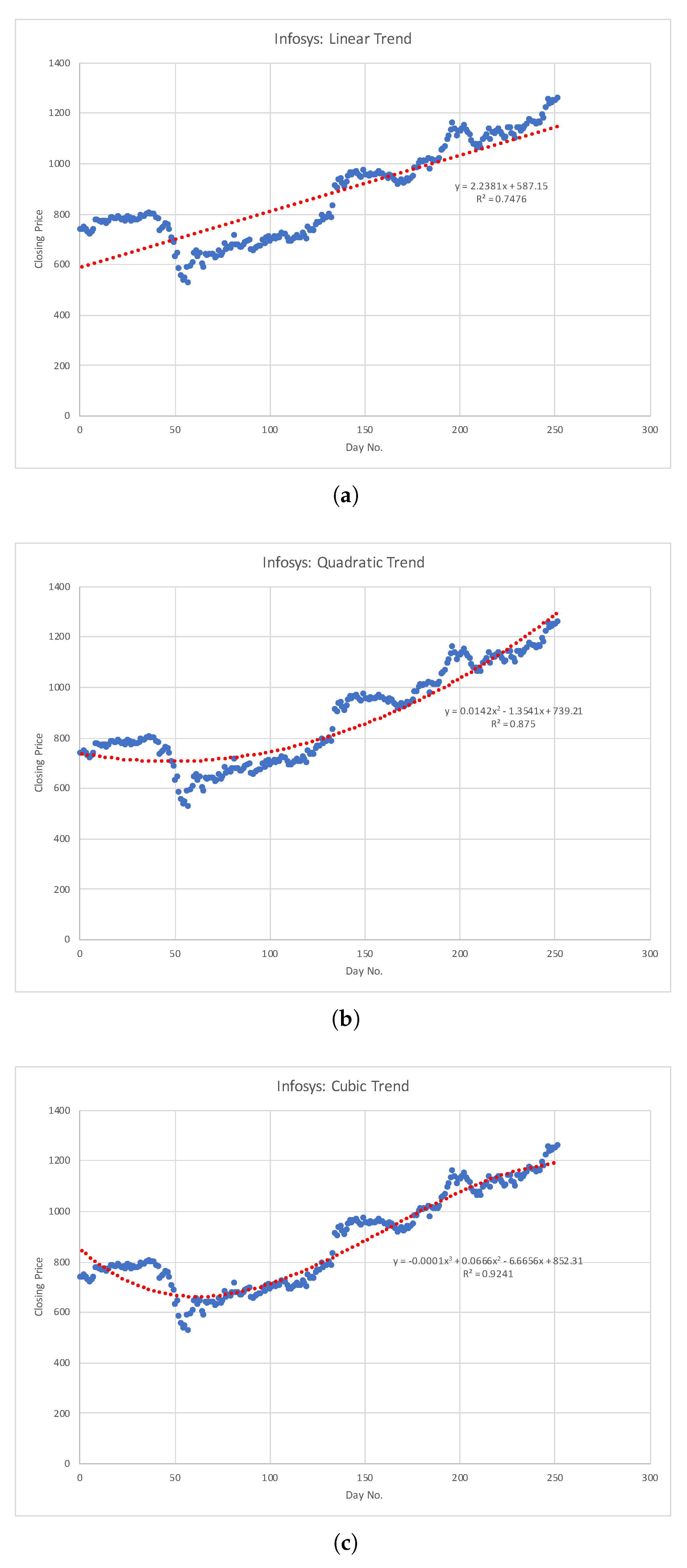
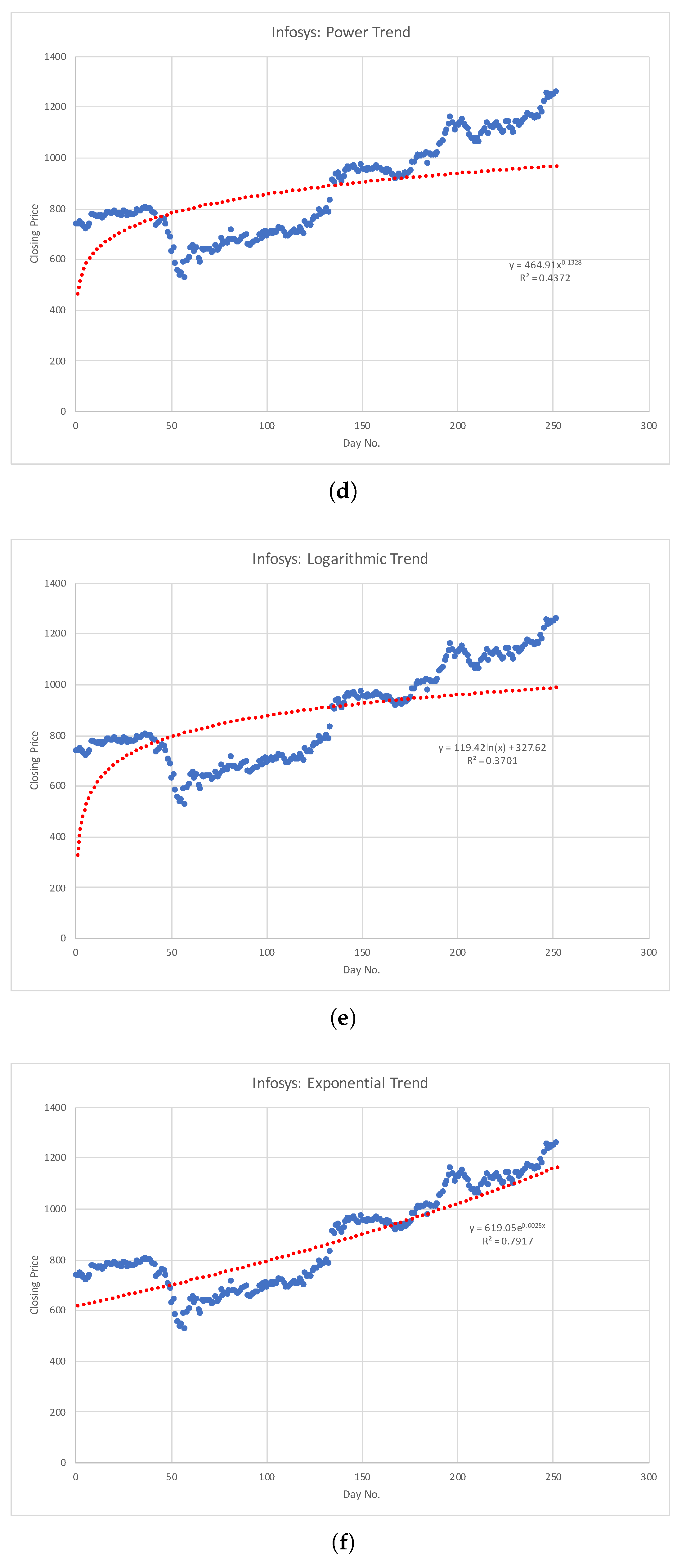
In our experiment, initially, we carried out regression on each company’s closing stock price from the initial data set and selected the curve of best fit.

As an example, in Figure 1, we show the different trend lines fitted with the closing stock prices of Infosys (Software sector) for the period from 1 January 2020 to 31 December 2020.

The equation of the fitted trend line, R-squared error, and RMS Error were calculated and presented in

Table 1. Best fit curve and RMSE for Infosys (Software sector).

Curve Trend	Equation	R-Squared Error	RMS Error
Linear	$2.2381x+587.15$	0.7476	513.3750
Quadratic	$0.0142x^2-1.3541x+739.21$	0.875	547.8658
Cubic	$-0.0001x^3+0.0666x^2-6.6656x+852.31$	0.9241	491.2556
Logarithmic	$119.42lnx+327.62$	0.3701	678.6604
Exponential	$619.05e^{0.0025x}$	0.7917	569.2302

. The curve of best fit is the one for which the RMS Error is minimum. The same process was carried out for all the 20 companies, but for sake of brevity, we display only one.

Our initial data are based on closing stock price of all the selected companies from 1 January 2021 to 31 December 2021 which comprises of total 252 working days in Indian stock market. Further, our evaluation and comparison period for the experiment is from 1 January 2021 to 18 October 2021, which comprises 196 working days. Thus, we find our predicted stock price for the 448th day (252 + 196 = 448) using regression. The best fit curve for each company along with its CNGR and predicted stock price was listed in

Table 2. Curve of best fit and CNGR of the companies.

Sl. No.	Sector	Company Name	Curve of	CNGR	Predicted Stock	Actual Stock Price
			Best Fit		Price on 18 October 2021	on 18 October 2021
1	Pharma	Dr. Reddy’s Lab	Quadratic	4.30124	6285.76	4877.50
2	Pharma	Sun Pharmaceuticals	Cubic	2.6818	742.52	835.90
3	Pharma	Divi’s Lab	Exponential	2.1625	6109.40	5343.05
4	Pharma	Cipla	Cubic	3.5268	1222.58	903.75
5	Software	Infosys	Cubic	4.528	2244.01	1792.15
6	Software	TCS	Cubic	2.534	3142.50	3647.15
7	Software	HCL	Quadratic	3.24	2459.83	1221.40
8	Software	Wipro	Cubic	4.512	612.78	709.75
9	Petro	Reliance Ind.	Exponential	3312.18	2888.44	2707.60
10	Petro	BPCL	Power	2.1074	583.27	462.50
11	Petro	ONGC	Quadratic	1.9271	181.75	162.10
12	Petro	Indian Oil Corp.	Cubic	1.524	101.35	136.35
13	Bank	HDFC	Exponential	4.109	1572.59	1670.30
14	Bank	ICICI	Exponential	2.1034	601.33	745.45
15	Bank	Kotak Mahindra	Exponential	2.5221	2172.72	2011.60
16	Bank	SBI	Power	4.212	253.86	497.95
17	Metal	Hindalco	Power	2.014	309.56	542.80
18	Metal	SAIL	Quadratic	2.84	89.91	129.0
19	Metal	Tata Steel	Exponential	3.1244	905.45	1411.05
20	Metal	Hindustan Zinc	Exponential	2.0127	314.52	387.65

.

Next, we perform the allocation of funds into multiple sectors by taking the mean of CNGR computed in Table 2 for each sector. This allocation is presented in

Table 3. Sector wise fund allocation.

Sl.	Sector	Sector	% of Fund Allocated	Amount (Approx.) of Fund Allocated
No.		Growth Rate (${\mathit{G}}_{\mathit{i}}$)	to a Sector (${\mathit{SP}}_{\mathit{i}}={\mathit{G}}_{\mathit{i}}\times \mathit{SMF}$)	to Sector (${\mathit{SF}}_{\mathit{i}}=\mathit{F}\times {\mathit{SP}}_{\mathit{i}}$) (in Rs.)
1	Pharma	3.1606	20.6482	20,648
2	Software	3.7035	24.1949	24,195
3	Petro	2.7074	17.687	17,688
4	Bank	3.2367	21.145	21,145
5	Metal	2.4977	16.3174	16,317

.

In

Table 4. Allocation of fund within companies.

Sl. No.	Sector	Company Name	Sector Fund	Company Growth Rate (${\mathit{g}}_{\mathit{i}}$)	CMF	% of Sector Fund Allocated to the Company (${\mathit{CP}}_{\mathit{i}}={\mathit{g}}_{\mathit{i}}\times \mathit{CMF}$)	Amount of Fund (in Rs.) (${\mathit{SF}}_{\mathit{i}}\times {\mathit{CP}}_{\mathit{i}}$)
1	Pharma	Dr. Reddy’s Lab	20,600	4.30124	7.8911	33.941	6992
2		Sun Pharmaceuticals		2.6818		21.1629	4360
3		Divi’s Lab		2.1625		17.0650	3515
4		Cipla		3.5268		27.83	5733
5	Software	Infosys	24,200	4.528	6.7503	30.5653	7397
6		TCS		2.534		17.1052	4134
7		HCL		3.24		21.87	5292
8		Wipro		4.512		30.4573	7371
9	Petro	Reliance Ind.	17,700	5.2712	9.2337	48.6726	8615
10		BPCL		2.1074		19.459	3444
11		ONGC		1.9271		17.795	3150
12		Indian Oil Corp.		1.524		14.0721	2491
13	Bank	HDFC	21,100	4.109	7.7239	31.739	6697
14		ICICI		2.1034		16.2464	3428
15		Kotak Mahindra		2.5221		19.48106	4111
16		SBI		4.212		32.533	6864
17	Metal	Hindalco	16,300	2.014	10.0089	20.1579	3286
18		SAIL		2.84		28.4252	4633
19		Tata Steel		3.1244		31.2718	5097
20		Hindustan Zinc		2.0127		20.1449	3284

, we provide the allocation of fund to each company based on their expected returns. It may be noted that Table 3 and Table 4 are exactly similar to those in Debnath and Srivastava (2021), since we are using the same methodology for allocation of fund.

We assume that the allocated funds remain invested throughout the period from 1 January 2021 to 18 October 2021.

We further assume that no stocks were bought or sold during this entire period.

In

Table 5. Absolute % return from 1 January to 18 October 2021.

Sl. No.	Sector	Company Name	Closing Price on 1 January 2021	Closing Price on 18 October 2021	Absolute % Return in This Period	Return from Allocated Fund (in Rs.)	Average Sector Absolute % Return
1	Pharma	Dr. Reddy’s Lab	5241.35	4877.50	−6.94	−485	21.34
2		Sun Pharmaceuticals	596.25	835.90	40.19	1752
3		Divi’s Lab	3849.05	5343.05	38.81	1372
4		Cipla	826.6	903.75	9.33	535
5	Software	Infosys	1260.45	1792.15	42.18	3120	44.52
6		TCS	2928.25	3647.15	24.55	1015
7		HCL	950.5	1221.40	28.50	1508
8		Wipro	388.1	709.75	82.87	6108
9	Petro	Reliance Ind.	1987.5	2707.60	36.23	3121	45.06
10		BPCL	381.95	462.50	21.08	726
11		ONGC	93.2	162.10	73.92	2328
12		Indian Oil Corp.	91.5	136.35	49.01	1221
13	Bank	HDFC	1425.05	1617.30	17.20	1152	34.40
14		ICICI	527.5	745.45	41.31	1416
15		Kotak Mahindra	1994.05	2011.60	0.88	36
16		SBI	279.4	497.95	78.22	5369
17	Metal	Hindalco	238.35	542.80	127.73	4197	95.61
18		SAIL	74.5	129.00	73.15	3389
19		Tata Steel	643.10	1411.05	119.41	6086
20		Hindustan Zinc	239.05	387.65	62.16	2041

, we present the absolute percentage return from each company which in turn gives us the absolute percentage return from each sector. This table is used for our evaluation and further comparison of performance with benchmark indices and several mutual funds.

5. Paired t-Test between the Performance in 2019 and 2021 and Comparison with Other Benchmark Indices

Now, we perform a comparative study between Table 5 and

Table 6. Absolute % return from 1 January to 31 December 2019.

Sl. No.	Sector	Company Name	Closing Price on 1 January 2019	Closing Price on 31 December 2019	Absolute % Return in This Period	Return from Allocated Fund (in Rs.)	Average Sector Absolute % Return
1	Pharma	Dr. Reddy’s Lab	2608.00	2869.55	10.03	701	6.39
2		Sun Pharmaceuticals	432.70	432.55	−0.34	−15
3		Divi’s Lab	1477.00	1838.15	24.45	859
4		Cipla	522.75	477.90	−8.57	−491
5	Software	Infosys	665.05	732.00	10.06	744	−10.55
6		TCS	1905.90	2165.00	13.59	562
7		HCL	960.00	569.00	−40.72	−2155
8		Wipro	328.70	246.10	−25.13	−1852
9	Petro	Reliance Ind.	1987.5	2707.60	35.29	3040	11.68
10		BPCL	368.50	491.45	33.36	1149
11		ONGC	148.25	128.55	−13.28	−418
12		Indian Oil Corp.	137.60	125.70	−8.64	−215
13	Bank	HDFC	2149.00	1275.50	−40.64	−2721	13.84
14		ICICI	364.20	538.65	47.89	1641
15		Kotak Mahindra	1249.00	1685.00	34.90	1434
16		SBI	300.70	333.80	11.24	771
17	Metal	Hindalco	222.90	215.80	−3.1	−102	−14.81
18		SAIL	55.70	42.95	−22.89	−1060
19		Tata Steel	515.60	470.75	−8.69	−443
20		Hindustan Zinc	277.95	209.70	−24.56	−806

. By X, we denote the random variable representing average sector-wise absolute % return in Table 6, i.e., for the year 2019, whereas by Y we denote the random variable representing average sector-wise absolute % return in Table 5, i.e., for the year 2021. For predicting stock prices in 2021, we have used stock prices from 1 January 2020 to 31 December 2020 as our initial data set. It would be interesting to know how the same portfolio would have performed in the year 2019 (i.e., we want to study the performance of the same scrips in 2019 if the same portfolio is blindly adopted without applying the selection methodology). Since the same set of scrips are used in both the cases, the readings X and Y are not independent, but they are paired together, and we apply the paired t-test for testing the null hypothesis $H_0$ and the alternative hypothesis $H_a$. Let ${\mu }_X$ denote the mean of X, and ${\mu }_Y$ denote the mean of Y.

Under $H_0:{\mu }_X={\mu }_Y$, i.e., there is no significant difference between the means. In addition, we have $H_a:{\mu }_Y>{\mu }_X$, and the test statistic is $t=\frac{\overline{d}}{S/\sqrt{n}}\sim t_{(n-1)}$, where $S^2=\frac{1}{n-1}\left[\sum d^2-\frac{{(\sum d)}^2}{n}\right]$ and $\overline{d}=\frac{\sum d}{n}$.

Hence, from

Table 7. Paired t-test using Table 5 and Table 6.

	X	Y	$\mathit{d}=\mathit{X}-\mathit{Y}$	${\mathit{d}}^2$
Pharma	6.39	21.34	−14.95	223.50
Software	−10.55	44.52	−55.07	3032.70
Petroleum	11.68	45.06	−33.38	1114.22
Bank	13.84	34.40	−20.56	422.71
Metal	−14.81	95.61	−110.42	12,192.57
			$\sum d=-234.38$	$\sum d^2=\mathrm{16,985.7}$

, we have $\overline{d}=\frac{-234.38}{5}=-46.876(n=5)$ and $S^2=1499.73$.

Further,

$$\left|t\right|=\frac{|\overline{d}|}{S/\sqrt{n}}=2.70.$$

However, the tabulated $t_{0.05}$ for $(5-1)=4$ degrees of freedom for one tailed test is 2.132. Since the calculated value of t is higher than the tabulated value, we reject the null hypothesis, and it implies that the observed value of t is significant at a 5% level of significance. We can conclude that the selection of scrips according to our proposed methodology significantly resulted in the superior performance of the same portfolio in 2021.

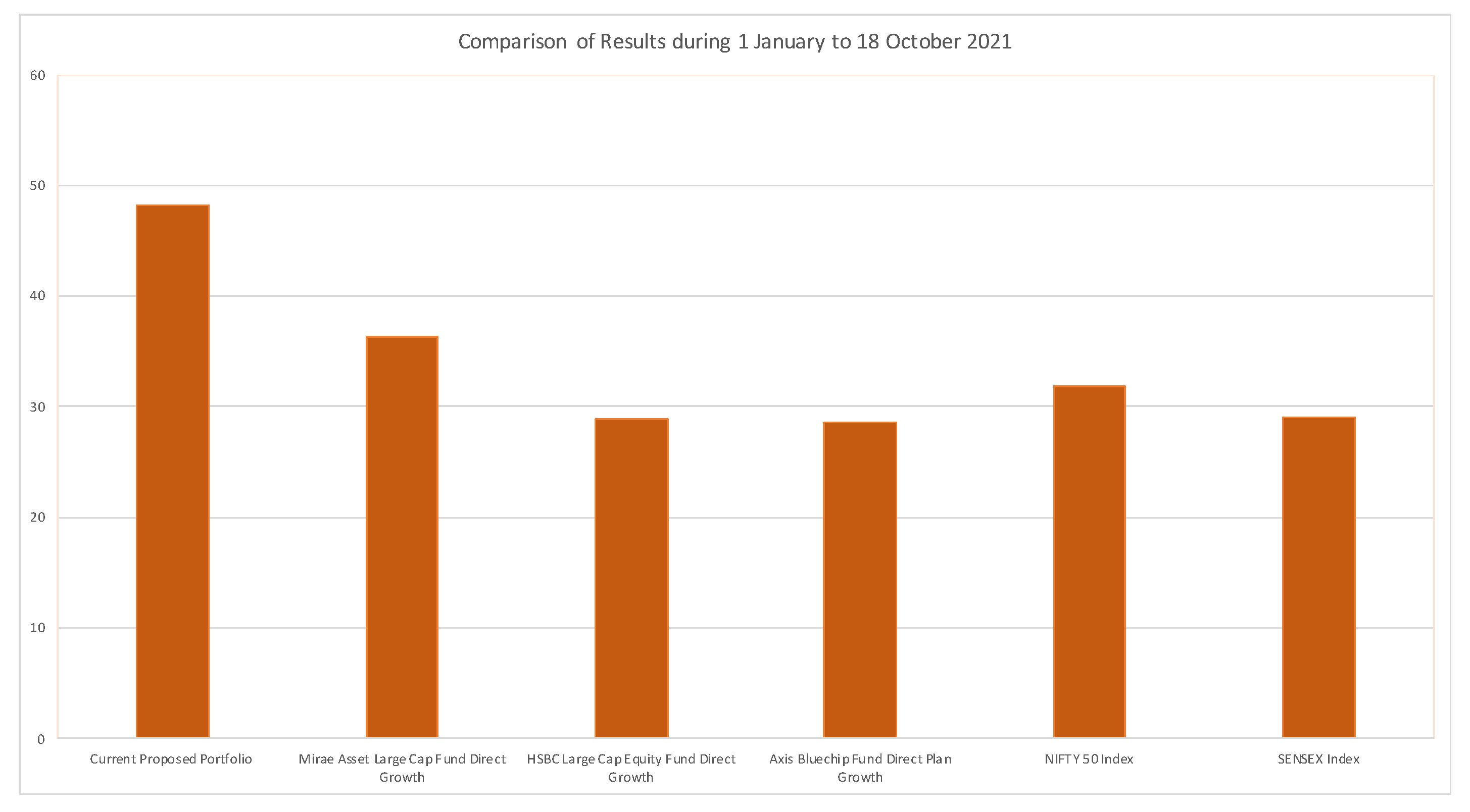
Next, we compare the performance of our proposed portfolio with some popular mutual funds which have been rendering high returns over the years (presented in

Table 8. Comparison of the performance of the proposed portfolio with benchmark indices.

Time	Absolute Return by Our	Absolute Return by Mirae	Absolute Return by HSBC	Absolute Return by Axis	NIFTY	SENSEX
Period	Current Proposed Portfolio (%)	Asset Large Cap Fund Direct Growth (%)	Large Cap Equity Fund Direct Growth (%)	Bluechip Fund Direct Plan Growth (%)	50 Index (%)	Index (%)
1 January 2021 to 18 October 2021	48.18	36.36	28.88	28.64	31.80	29.03

and Figure 2). The performance data of the mutual funds in the said period were collected from their respective web portals. The absolute percentage return by our proposed portfolio is found to be $21.78$ which is the average of the ’average sector absolute % return’ as given in Table 5.

We can observe that our proposed portfolio performed quite excellently during this period with an absolute return of 48.18% which was 21.78% during 1 January 2021 to 21 May 2021. Our proposed portfolio also outperformed benchmark indices such as NIFTY 50 and SENSEX and several popular mutual funds in this period.

6. Conclusions

This work is an extended version of Debnath and Srivastava (2021) with certain new contributions. A comparative study was performed in Section 5 to validate the sustainability of the model post-second wave of COVID-19 in India. In addition, it was shown that the model may not produce the expected outcome if adopted arbitrarily without following the stock selection methodology. For this purpose, we performed paired t-test for the significance of difference of sector-wise mean returns in the year 2019 and 2021. We found that the application of our proposed methodology for selection of stocks significantly enhanced the sector-wise mean returns in the year 2021.

We further compared the performance of our portfolio with benchmark indices such as NIFTY 50 and SENSEX and observed that our portfolio gave better returns than those indices. In our previous work, which was for the period from 1 January 2021 to 21 May 2021, this portfolio gave an absolute return of 21.78%, whereas for the current period of 1 January 2021 to 18 October 2021, it has provided an absolute return of 48.18%. These data are tabulated in Table 8, and the graphical comparison is shown in Figure 2. It can also be observed that our portfolio beat the performance of several popular mutual funds in the current period as well.

7. Future Work

The current work is of interest to portfolio managers as well as retailers considering the present scenario in the Indian stock market. However, we believe our work is not free from limitations. In this regard, we suggest some future work that will certainly improve the portfolio returns and reveal new research directions. An extension of Table 6 to cover not just absolute returns in different sectors but the associated deviation and risk measures such as standard deviation, CVaR 95% and CVaR99% using the frame work of Allen et al. (2012); Cheridito and Kromer (2013) would be of immense interest to researchers. Additionally, the corresponding risk-adjusted performance ratios may also be covered. The performance, sustainability, and sustainability assessment are also key foci these days, see Popescu (2020). The inclusion of these factors will greatly enhance the studies in market research.

References

- Al-Awadhi, Abdullah M., Khaled Al-Saifi, Ahmad Al-Awadhi, and Salah Alhamadi. 2020. Death and contagious infectious diseases: Impact of the Covid-19 virus on stock market returns. Journal of Behavioral and Experimental Finance 27: 100326. [Google Scholar] [CrossRef]
- AlArjani, Ali, Md. Maniruzzaman Miah, Md. Sharif Uddin, Abu Hashan Md Mashud, Hui-Ming Wee, Shib Sankar Sana, and Hari Mohan Srivastava. 2021. A sustainable economic recycle quantity model for imperfect production system with shortages. Journal of Risk and Financial Management 14: 173. [Google Scholar] [CrossRef]
- Albulescu, Claudiu Tiberiu. 2020. Covid-19 and the United States’ financial market’s volatility. Finance Research Letters 38: 101699. [Google Scholar] [CrossRef]
- Allen, David Edmund, Robert J. Powell, and Abhay Kumar Singh. 2012. Beyond reasonable doubt: Multiple tail risk measures applied to European industries. Applied Economics Letters 19: 671–76. [Google Scholar] [CrossRef]
- Altay, Erdinc, and M. Hakan Satman. 2005. Stock market forecasting: Artificial neural network and linear regression comparison in an emerging market. Journal of Financial Management and Analysis 18: 18. [Google Scholar]
- Atsalakis, George S., and Kimon P. Valavanis. 2009. Surveying stock market forecasting techniques: Soft Computing Methods. Expert Systems with Applications 36: 5932–41. [Google Scholar] [CrossRef]
- Baralis, Elena, Luca Cagliero, and Paolo Garza. 2017. Planning stock portfolios by means of weighted frequent itemsets. Expert Systems with Applications 86: 1–17. [Google Scholar] [CrossRef]
- Cheridito, Patrick, and Eduard Kromer. 2013. Reward-Risk Ratios. Journal of Investment Stragies. [Google Scholar] [CrossRef]
- Debnath, Pradip, and Hari M. Srivastava. 2021. Optimizing stock market returns during global pandemic using regression in the context of Indian stock market. Journal of Risk and Financial Management 14: 386. [Google Scholar] [CrossRef]
- Engelhardt, Nils, Miguel Krause, Daniel Neukirchen, and Peter Posch. 2020. What drives stocks during the Corona-crash? News attention vs. rational expectation. Sustainability 12: 5014. [Google Scholar] [CrossRef]
- Erdem, Orhan. 2020. Freedom and stock market performance during covid-19 outbreak. Finance Research Letters 36: 101671. [Google Scholar] [CrossRef]
- Gottschlich, Jorg, and Oliver Hinz. 2014. A decision support system for stock investment recommendations using collective wisdom. Decision Support Systems 59: 52–62. [Google Scholar] [CrossRef]
- Liao, Shu-Hsien, Pei-Hui Chu, and Pei-Yuan Hsiao. 2012. Data mining techniques and applications—A decade review from 2000 to 2011. Expert Systems with Applications 39: 11303–11. [Google Scholar] [CrossRef]
- Maji, Giridhar, Debomita Mondal, Nilanjan Dey, Narayan C. Debnath, and Soumya Sen. 2021. Stock prediction and mutual fund portfolio management using curve fitting techniques. Journal of Ambient Intelligence and Humanized Computing, 1–14. [Google Scholar] [CrossRef]
- Mazur, Mieszzko, Man Dang, and Miguel Vega. 2020. COVID-19 and the march 2020 stock market crash. Evidence from S&P1500. Finance Research Letters 38: 101690. [Google Scholar] [CrossRef] [PubMed]
- Paranjape-Voditel, Preeti, and Umesh Deshpande. 2013. A stock market portfolio recommender system based on association rule mining. Applied Soft Computing 13: 1055–63. [Google Scholar] [CrossRef]
- Popescu, Cristina Raluca Gh. 2020. Sustainability Assessment: Does the OECD/G20 Inclusive Framework for BEPS (Base Erosion and Profit Shifting Project) Put an End to Disputes Over The Recognition and Measurement of Intellectual Capital? Sustainability 12: 10004. [Google Scholar] [CrossRef]
- Rahman, Md Lutfur, Abu S. Amin, and Mohammed Abdullah Al Mamun. 2021. The COVID-19 outbreak and stock market reactions: Evidence from Australia. Finance Research Letters 38: 101832. [Google Scholar] [CrossRef]
- Rusu, Virginia, and Cristian Rusu. 2003. Forecasting methods and stock market analysis. Creative Mathematics 12: 103–10. [Google Scholar]
- Takahashi, Hidenori, and Kazuo Yamada. 2020. When Japanese stock market meets Covid-19. Impact of ownership, trading, esg, and liquidity channels. SSRN Electronic Journal. [Google Scholar] [CrossRef]
- Zaremba, Adam, Renatas Kizys, David Y. Aharon, and Ender Demir. 2020. Infected Markets: Novel coronavirus, Government interventions, and stock return volatility around the globe. Finance Research Letters 35: 101597. [Google Scholar] [CrossRef] [PubMed]
- Zhang, Dayong, Min Hu, and Qiang Ji. 2020. Financial markets under the global pandemic of COVID-19. Finance Research Letters 36: 101528. [Google Scholar] [CrossRef] [PubMed]
Figure 1.
Trend lines for Infosys (Software Sector): January–December 2020. (a) Linear; (b) Quadratic; (c) Cubic; (d) Power; (e) Logarithmic; (f) Exponential.
Figure 2.
Comparison of the performance of the proposed portfolio with benchmark indices.