Sticky Stock Market Analysts

Abstract

Technological progress in recent years has made new methods available for making forecasts in a variety of areas. We examine the success of ex-ante stock market forecasts of three major stock market indices, i.e., the German Stock Market Index (DAX), the Dow Jones Industrial Index (DJI), and the Euro Stoxx 50 (SX5E). We test whether the forecasts prove true when they reach their effective dates and are therefore suitable for active investment strategies. We revive the thoughts of the American sociologist William Fielding Ogburn, who argues that forecasters consistently underestimate the variability of the future. In addition, we draw on some contemporary measures of forecast quality (prediction-realization diagram, test of unbiasedness, and Diebold–Mariano test). We reveal that (a) unusual events are underrepresented in the forecasts, (b) the dispersion of the forecasts lags behind that of the actual events, (c) the slope of the regression lines in the prediction-realization diagram is <1, (d) the forecasts are highly biased, and (e) the quality of the forecasts is not significantly better than that of naïve forecasts. The overall behavior of the forecasters can be described as “sticky” because their forecasts adhere too strongly to long-term trends in the indices and are thus characterized by conservatism.

1. Introduction

Capital market forecasts often show a closer connection to the capital market development of the present than to the capital market development of the future. This phenomenon is known as topically orientated trend adjustment (Andres and Spiwoks 1999). It occurs equally in share price forecasts, interest rate forecasts, exchange rate forecasts, and commodity price forecasts (see, e.g., Filiz et al. 2019; Kunze et al. 2018; Spiwoks et al. 2015; Spiwoks and Hein 2007). A tendency to underestimate the variability of reality could be an important cause (Spiwoks et al. 2015).

The American sociologist William Fielding Ogburn discovers almost 90 years ago that forecasters systematically underestimate the actual variability of reality (Ogburn 1934). He provides a concrete research approach to identify such behavior. Presumably because Ogburn deals with the prognosis of sporting events and not with the prognosis of economic events, he has so far not been noticed by economic research.

During an empirical analysis of the forecasting behavior of experts and lay people, Ogburn (1934) concludes that the variability of reality is consistently underestimated. He traces this back to a tendency which he calls the “conservatism of the predictors”. In detail, he is referring to:

• Unusual events (e.g., a sudden drop in an otherwise rising trendline) are forecasted more seldom than they occur in reality, whereas normal events (e.g., a recently rising trendline continuing to rise) are over-represented in forecasts.
• The standard deviation of the forecasts is lower than the standard deviation of the actual events.
• The extent of the forecasted changes lags behind the scale of the actual changes.

Active investment strategies have been popular since the emergence of modern stock markets (Maxwell and van Vuuren 2019; Lofthouse 1996; Friend and Vickers 1965; Cowles 1933). In order to successfully design active investment strategies such as market timing, stock picking, or index picking, forecasts of future stock market developments are indispensable. New forecasting methods are constantly being discussed: econometric models (Goyal et al. 2021; Chen and Vincent 2016; Welch and Goyal 2008), artificial neural networks (Rajab and Sharma 2019; Atsalakis and Valavanis 2009), artificial intelligence (Mallikarjuna and Rao 2019), capital market simulations with multi-agent models (Yang et al. 2020; Krichene and El-Aroui 2018; Arthur et al. 1997), modelling based on the expectations of capital market agents (Atmaz et al. 2021; Greenwood and Shleifer 2014), and neuro-psycho-economics approaches (Ortiz-Teran et al. 2019; Kandasamy et al. 2016; Werner et al. 2009). However, testing these approaches using ex-post forecasts in an out-of-sample data domain repeatedly leads to apparent forecasting successes that then may not materialize in real ex-ante settings (Kazak and Pohlmeier 2019). When the variability of reality is systematically underestimated, this can contribute towards very costly errors in the field of stock market forecasts. Under certain circumstances, basing active investment strategies on inappropriate stock market forecasts can lead to serious losses and even bankruptcy, when expected returns do not occur. Due to the necessity of reliable forecasts for a successful active investment strategy, stock market forecasting is a dynamic field of research.

The reliability of stock market forecasts is rarely examined. There are many studies on pre-tax profit forecasts (Ramnath et al. 2008), but research on the success of actual ex-ante forecasts in stock prices, stock market indices, or stock market returns are still a rarity. So far, it has not been in the focus of research whether stock market forecasts are characterized by a systematic underestimation of the variability of reality as found by Ogburn (1934). This research gap is even more surprising because the necessary investigation tools have long been available in the form of Theil’s prediction-realization diagram and the test for unbiasedness. We raise the question of how successful experts were in forecasting major stock indices (DAX, Dow Jones Industrial Index, Euro Stoxx 50) in the period from 1992 to 2020. We use Ogburn’s (1934) examination instruments. But we also go beyond this and use current standard procedures such as the comparison to the naïve forecasts (Diebold–Mariano test) and the unbiasedness test.

The forecasts turn out to be quite unreliable. Indeed, forecasters underestimate the variability of reality. This offers interesting starting points for improving the forecasting process.

2. Literature Review

2.1. Technological Progress in Stock Market Forecasting

There is a rich literature on the appliance of advanced econometric methodology in the forecasting process in order to identify meaningful predictors for future events. Guo (2006) uses ordinary and dynamic least squares regressions to analyze whether four different variables can be used as predictors for stock returns. The study concludes that the consumption-wealth ratio can indeed be used for statistically significant forecasts. Chen and Vincent (2016) also use different econometric models applied to full-sample approaches and out-of-sample approaches in order to analyze the informational value of different variables for the development of the Standard and Poor’s 500 index (S&P 500) for the period 1964 to 2011. They conclude that the market momentum and the investor sentiment can indeed serve as potential predictors for bear markets. In a similar study, Neely et al. (2014) find that adding technical variables to the commonly used macroeconomic predictors can significantly improve the quality of forecasts for the equity risk premium.

Welch and Goyal (2008) examine the informative value of 13 frequently used variables such as dividend yields or inflation. In contrast to the researchers mentioned above, they find that none of the 13 variables can be used to predict the S&P 500 index returns from 1926 to 2004 neither in-sample nor out-of-sample. Quite importantly, they also find that none of the information available at the time of a potential investment decision would have helped to gain an idea of future developments. A couple of years later, the same authors extend their research to 29 additional variables that have been brought up in the discussion in the meantime. In spite of the advances in research methods, they still diagnose a poor usefulness in predicting the equity premium in-sample and out-of-sample (Goyal et al. 2021).

Bahrami et al. (2018) add to the research by finding that even though most variables themselves do not lead to significant forecasts, combining forecasts from individual predictive models significantly improves the quality of stock return forecasts for ten advanced emerging markets across the globe.

Whereas most studies cited above apply OLS regression models, Nyberg (2013) examines the suitability of dynamic binary time series models for predicting the S&P 500 index between 1957 and 2010. The author concludes that both in-sample and out-of-sample, dynamic binary time series models are able to successfully forecast bull and bear markets.

A very dynamic research area is capital market simulation with multi-agent models. Heterogeneous agents interact with one another on an artificial stock market. Their demand for shares and their supply of shares are brought together in a stock exchange, so that the development of the share prices results from the actions of the individual agents. These in turn observe the development of the share price and adjust their further behavior to the development of the share price. In this way, the special dynamics of interactions on stock markets can be modeled and examined more closely. The artificial stock markets are validated using the stylized facts (e.g., fat tails, gain-loss asymmetry, volatility clustering, volume-volatility correlation). The price patterns of artificial stock markets should correspond to the price patterns of real stock markets.

The first highlight of this research area is the Santa Fe Artificial Stock Market (Arthur et al. 1997). The Frankfurt Artificial Stock Market (Hein et al. 2012) also takes into account a realistic stock exchange mechanism, different communication structures between the agents, and different investment philosophies of the agents. Recently, for example, information asymmetries (Krichene and El-Aroui 2018), memory length and confidence level (Bertella et al. 2014), risk preference (Chen and Huang 2008), tick size systems (Yang et al. 2020), and different types of stocks (Ponta and Cincotti 2018) have been taken into account in artificial stock markets. Artificial stock markets have the significant advantage that extreme events (crashes) can be observed more frequently and can be better analyzed than on real stock markets. The decisive disadvantage of the artificial stock markets is that the models are still too abstract to lead to very concrete share price forecasts.

Another very dynamic research area uses survey data to examine the expectations of capital market players more closely (e.g., Atmaz et al. 2021; Cassella and Gulen 2019; Cassella and Gulen 2018; Greenwood and Shleifer 2014). In some approaches, different types of investors (lay people vs. professionals or contrarians vs. extrapolators) are taken into account. The different expectations of these investor groups are then used to develop models for describing or forecasting share price developments. These approaches appear particularly promising because the special importance of the expectations for capital market events is emphasized. In addition, real capital market data are linked with survey data on the expectations of capital market players in a very differentiated manner. In contrast to the approaches of capital market simulation based on multi-agent models, these research approaches remain close to the observable reality of price formation on the stock markets.

In recent years, there have also been promising results regarding neuro-fuzzy systems used for stock price forecasting. For example, Atsalakis and Valavanis (2009) create a neuro-fuzzy system that outperforms a traditional “buy and hold”-strategy regarding the Athens and the New York Stock Exchange. Even in a direct comparison to econometric methods, Rajab and Sharma (2019) show that neuro-fuzzy approaches to forecasting the Bombay Stock Exchange, CNX Nifty, and S&P 500 can significantly outperform multiple regression analysis models or generalized autoregressive conditional heteroscedasticity models.

On the other hand, Mallikarjuna and Rao (2019) find that traditional linear and non-linear models are more accurate at forecasting daily stock market returns of selected indices from developed, emerging, and frontier markets for the period 2000 to 2018 than newly emerged artificial intelligence and frequency domain models. However, neither of the four models nor hybrid approaches provide satisfying results across the markets in their study.

In the field of neuro-psycho-economic approaches, Kandasamy et al. (2016) show that interoception, i.e., the perception of physiological signals from within the body, seems to play a role in the success of professional financial traders. Werner et al. (2009) also show that people with good cardiac perception perform better when choosing between profit and loss options.

In the context of ex-post forecasts in the out-of-sample area, these approaches sometimes show enormous potential. However, many of these approaches have yet to prove their suitability for actual ex-ante forecasts. Their informative value for ex-ante forecasts might be limited due to, for example, differences in estimation risk and low statistical power (Kazak and Pohlmeier 2019).

2.2. Ex-Ante Stock Market Forecasts

The actual success of stock market forecasts is thus best checked against real ex-ante forecasts. In the area of interest rate forecasts, the evaluation of continuously published forecasts has a long tradition (Filiz et al. 2021; Fassas et al. 2021; Filiz et al. 2019; Kunze et al. 2017; Miah et al. 2016; Pierdzioch 2015; Baghestani et al. 2015; Oliver and Pasaogullari 2015; Spiwoks et al. 2015). In the area of stock market forecasting, however, there are only a small number of studies that check continuously published stock market forecasts for their reliability (see the synoptic overview in

Table 1. Synoptic overview of studies on ex-ante stock market forecasts.

Study	Subject of the Forecast	Methods	Time Scale	Result
Lakonishok (1980)	S&P 425	Unbiasedness test with Theil–Sen estimator, Theil’s U, turning point errors	1947–1974	−
Dimson and Marsh (1984)	Selected British shares	Comparison of forecast and actual return via t-test, Unbiasedness test	1980–1981	+
Fraser and MacDonald (1993)	CAC 40	Unbiasedness test, root mean squared error	1984–1987	−
Spiwoks (2004)	Dow Jones Industrial Index, DAX, FT-SE 100, CAC 40, MIBtel, and the Nikkei 225	Analysis of turning point errors, Theil’s U, TOTA coefficient	1994–2004	−
Benke (2006)	DAX	Comparison of absolute frequencies regarding forecasting errors, direction of error, and comparison to naïve forecasts without statistical test	1992–2005	−
Spiwoks and Hein (2007)	Dow Jones Industrial Index, DAX, FT-SE 100, CAC 40, MIBtel, and the Nikkei 225	Root mean squared relative error, mean absolute relative error	1994–2004	−
Bacchetta et al. (2009)	Dow Jones Industrial Index, and Nikkei 225	Log Regression	1998–2005	+
Fujiwara et al. (2013)	TOPIX	Augmented Dickey–Fuller test, ADF-Fisher chi-square test	1998–2010	−

+ = Overall, the forecasts are assessed as good; − = overall, the forecasts are assessed as being flawed.

).

Lakonishok (1980) analyzes forecasts for the S&P 425 index in the period from 1947 to 1974. He concludes that the reliability of the forecasts does not go recognizably beyond that of naïve forecasts. In this context, a naïve forecast is defined as the assumption that the prevailing value for the variable being forecast at the time the forecast is made will also prevail in the future. In addition, the forecasts are biased and systematically underestimate the returns of the S&P 425. Dimson and Marsh (1984) analyze the forecasted returns of 206 selected British shares in the period from 1980 to 1981. The authors conclude that the forecasts are successful and can lead to systematic excess returns. Fraser and MacDonald (1993) examine forecasts for the development of the French CAC 40 index in the period from 1984 to 1987. This reveals that the forecasts are less reliable than naïve forecasts. Furthermore, it is evident that the forecasts tend to be oriented towards the present rather than the future.

Spiwoks (2004) and Spiwoks and Hein (2007) consider forecasts for six international share indices (the Dow Jones Industrial Index, the DAX, the FT-SE 100, the CAC 40, MIBtel, and the Nikkei 225) issued in the period from 1994 to 2004. The results are very similar. Almost without exception, the forecast time series exhibit greater forecasting errors than the respective naïve forecast. In addition, they exhibit topically orientated trend adjustment (Andres and Spiwoks 1999). In other words, they reflect the present situation more than anything else, and hardly provide any insights into future trends.

Benke (2006) examines DAX forecasts for the period from 1992 to 2005. He establishes that the forecasters consistently underestimate the extent of the actual changes. Bacchetta et al. (2009) analyze forecasts for the Dow Jones Industrial Index and the Nikkei 225 in the period from 1998 to 2005. The authors conclude that the forecasts are suitable for achieving systematic excess returns. Fujiwara et al. (2013) observe TOPIX forecasts in the years from 1998 to 2010. They argue that the forecasters are too strongly orientated towards their previous forecasts and systematically underestimate the actual trends of the TOPIX.

As we want to consider the abilities of professional stock market analysts, experimental studies in which the subjects are asked to make stock market forecasts themselves (e.g., Theissen 2007; De Bondt 1993) are not considered here.

2.3. Hypotheses

Capital market forecasts often describe the present rather than the future. Spiwoks et al. (2015) cite the systematic underestimation of the variability of reality as a possible reason for the phenomenon of topically oriented trend adjustments in capital market forecasts. The American sociologist William Fielding Ogburn (1934) is the first to address the systematic underestimation of the variability of reality in predicting future events. He presumes that (1) unusual events (e.g., a sudden drop in an otherwise rising trendline) are forecasted too seldom, that (2) the standard deviation of the forecasts is lower than the standard deviation of the actual events, and that (3) the forecasted changes lag behind the actual changes.

We check whether the forecasts for the German Stock Market Index (DAX), the Dow Jones Industrial Index (DJI) and the Euro Stoxx 50 (SX5E) also show these three properties. In formulating the hypotheses, we assume that the observations made by Ogburn (1934) who investigated forecasts of sporting events also apply to stock market forecasts.

Unlike the DAX, the DJI and the SX5E are price indices. Nevertheless, their long-term development is considered to be non-stationary. Over the long term, a rising trend can be recognized in all three stock indices. To this extent, it is simple to define unusual and normal events. A normal event is an increase in the share price index. An unusual event is a decrease in the share price index. Hypotheses 1 and 2 are therefore:

Hypothesis 1.

Falls in stock market indices are forecasted more seldom than they occur in reality.

Hypothesis 2.

The standard deviation of the forecasted changes of the stock market indices is lower than the standard deviation of the actual changes in the indices.

Should the systematical underestimation of the variability of reality be true in our data basis, investors would be exposed to a high risk, as relatively large changes in trends, also negative ones, would not be reflected adequately in the forecasts. The best way to test this assumption is to compute a prediction-realization diagram (Theil 1958) that compares the forecasted relative share price changes to the actual relative share price changes (as described in the Methods section). If the forecast changes are smaller than the actual changes, this leads to a regression line with a slope of <1 in the prediction-realization diagram. Hypothesis 3 therefore reads:

Hypothesis 3.

The slope of the regression lines in the prediction-realization diagram is lower than one (slope < 1).

If the predicted changes lag behind the actual changes and it is thus true that the forecasters are guided by conservatism, the forecasts are not unbiased. This can be verified best by means of the test of unbiasedness using the Mincer–Zarnowitz regression (as described in the Methods section). The use of the unbiasedness test is of particular interest here because it can be used to determine whether the underestimation of the changes in the prognosis object can be viewed as statistically significant. Hypothesis 4 is therefore:

Hypothesis 4.

The forecasts prove to be biased.

An assessment of capital market forecasts is incomplete if the forecasts are not compared to the naïve forecasts. In view of the results of previous studies (Spiwoks and Hein 2007; Spiwoks 2004; Fraser and MacDonald 1993; Lakonishok 1980), we expect that the quality of the forecasts will not be significantly better than that of naïve forecasts. If this is the case, investors should by no means consider the forecasts, as the naïve forecast is readily available at any time. Hypothesis 5 is therefore:

Hypothesis 5.

The quality of the forecasts is not significantly higher than that of naïve forecasts.

3. Data Basis

We evaluate DAX forecasts which were published between 1992 and 2020 in the Handelsblatt newspaper (HB). The forecasts have a forecast horizon of one year. In addition, we evaluate forecasts for the DAX and the Euro Stoxx 50 which were published in the period from 2002 to 2020 in the Frankfurter Allgemeine Zeitung (FAZ). We also analyze forecasts for the Dow Jones Industrial Index which were published between 2004 and 2020 in the FAZ. The time scales differ as we have taken into account all stock price forecasts since the beginning of their publication in order to get more meaningful results. These forecasts have forecast horizons of six and twelve months (

Table 2. Data basis and summary statistics.

Source	Subject	Period	N	Min (in %)	Max (in %)	Median (in %)	Mean (in %)	N	Min (in %)	Max (in %)	Median (in %)	Mean (in %)
			Forecast Horizon 6 Months					Forecast Horizon 12 Months
HB	DAX	1992–2020	NA	NA	NA	NA	NA	964	−25.16	72.85	8.08	8.76
FAZ	DAX	2002–2020	282	−33.47	18.68	3.38	2.34	402	−25.16	45.20	8.14	8.94
FAZ	DJI	2004–2020	203	−21.45	23.06	1.62	1.39	259	−20.24	42.43	6.07	5.95
FAZ	SX5E	2002–2020	270	−34.63	22.57	3.24	2.32	381	−20.33	36.87	7.88	8.03
Σ			755					2006

HB = Handelsblatt; FAZ = Frankfurter Allgemeine Zeitung; DAX = German Stock Market Index; DJI = Dow Jones Industrial Index; SX5E = Euro Stoxx 50; N = number of forecasts issued; Min = minimum; Max = maximum; NA = not available.

). We provide the dataset used in our study as a Supplementary in an Excel format. The dataset comprises all analyzed forecasts published annually in the Frankfurter Allgemeine Zeitung and Handelsblatt between 1992 and 2020.

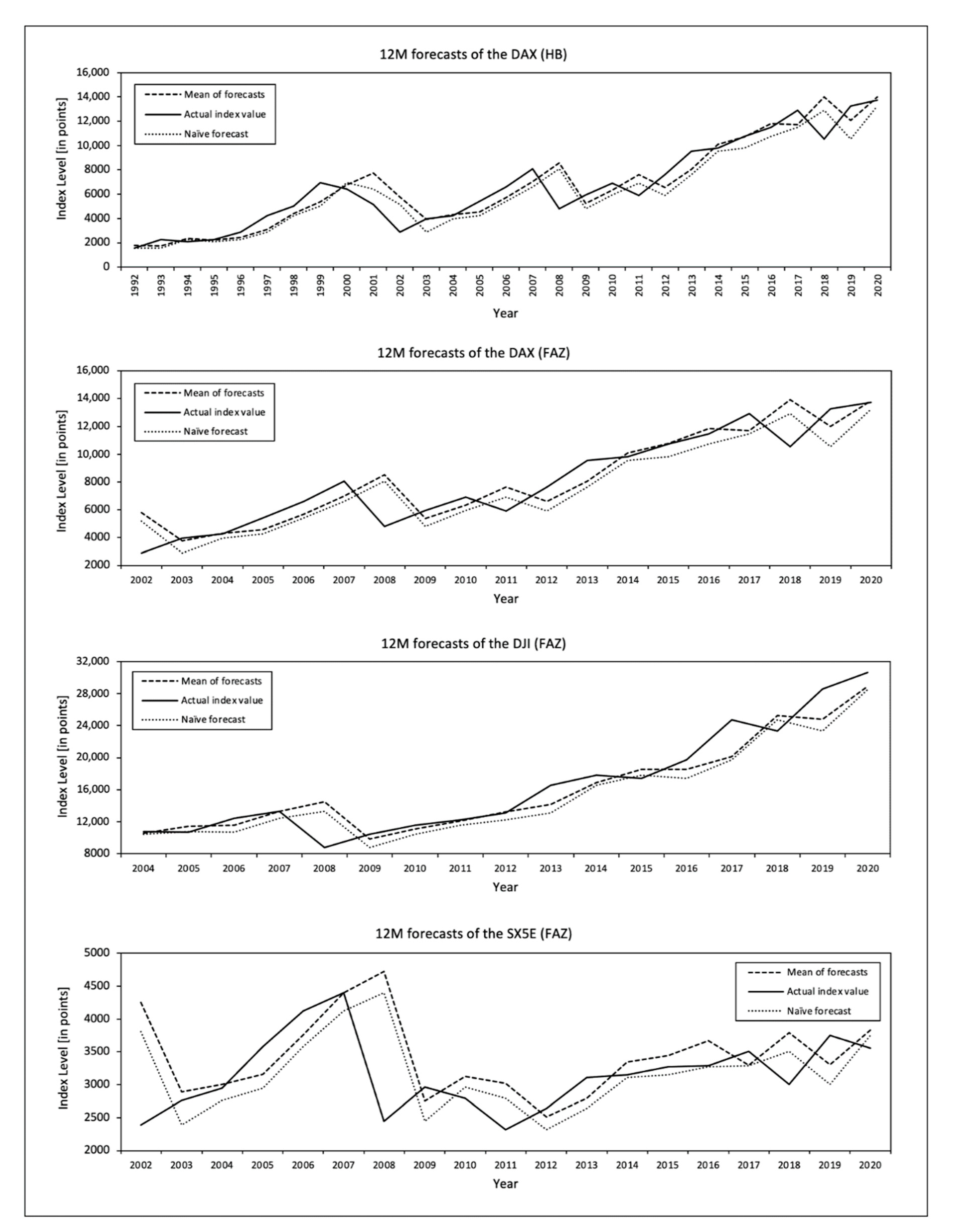
In Table 2, we also provide descriptive statistics and show both the minimum and maximum predicted percentage index level changes as well as the median and mean value of the predicted percentage index level changes for the examined data. The descriptive statistics on forecast index level changes in Table 2 are shown in percentages to give a clearer picture of the data. The institutes did not forecast percentage index level changes, but rather the respective index levels. For example, M.M. Warburg & Co. predicted the DAX index level at the end of the year 2009 at 3600 points. At the time the forecast was issued, the DAX had an index level of 4810.20 points. Thus, the institute forecast the largest price decline of 25.16%. The WGZ-Bank forecast the maximum percentage increase in the index level of the DAX in 2003. While the DAX had an index level of 2892.63 points at the time the forecast was made, the bank forecast a percentage increase of 72.85% to 5000 points at the end of the year. On average, the institutes forecast an index level increase of the DAX of 8.76% (median 8.08%) in the period considered from 1992 to 2020 (see

Table A1. Detailed Summary Statistics on DAX, DJI, and SX5E forecasts of our data basis.

Source	Subject	Year	N	Min [pts.]	Max [pts.]	Median [pts.]	Mean [pts.]	Actual [pts.]	N	Min [pts.]	Max [pts.]	Median [pts.]	Mean [pts.]	Actual [pts.]
			Forecast horizon 6 months						Forecast horizon 12 months
HB	DAX	1992	NA	NA	NA	NA	NA	NA	21	1600	1900	1780	1764	1545.05
		1993	NA	NA	NA	NA	NA	NA	25	1550	1900	1750	1726	2266.68
		1994	NA	NA	NA	NA	NA	NA	28	1840	2500	2400	2339	2106.58
		1995	NA	NA	NA	NA	NA	NA	33	1950	2500	2200	2225	2253.88
		1996	NA	NA	NA	NA	NA	NA	28	2250	2700	2450	2449	2888.69
		1997	NA	NA	NA	NA	NA	NA	34	2600	3800	3100	3095	4249.69
		1998	NA	NA	NA	NA	NA	NA	33	4000	4800	4413	4413	5002.39
		1999	NA	NA	NA	NA	NA	NA	34	4580	6000	5400	5390	6958.14
		2000	NA	NA	NA	NA	NA	NA	37	6200	7620	6790	6771	6433.61
		2001	NA	NA	NA	NA	NA	NA	33	6100	9000	7800	7722	5160.10
		2002	NA	NA	NA	NA	NA	NA	38	5100	6650	5750	5779	2892.63
		2003	NA	NA	NA	NA	NA	NA	33	3300	5000	3915	3921	3965.16
		2004	NA	NA	NA	NA	NA	NA	34	3500	5000	4300	4318	4256.08
		2005	NA	NA	NA	NA	NA	NA	33	4100	5000	4600	4558	5408.26
		2006	NA	NA	NA	NA	NA	NA	38	5000	6100	5800	5717	6596.92
		2007	NA	NA	NA	NA	NA	NA	37	6000	7500	7078	7027	8067.32
		2008	NA	NA	NA	NA	NA	NA	35	7700	9250	8500	8566	4810.20
		2009	NA	NA	NA	NA	NA	NA	31	3600	6500	5250	5230	5957.43
		2010	NA	NA	NA	NA	NA	NA	38	4500	7500	6345	6339	6914.19
		2011	NA	NA	NA	NA	NA	NA	39	6200	8300	7600	7605	5898.35
		2012	NA	NA	NA	NA	NA	NA	37	5500	7600	6573	6573	7612.39
		2013	NA	NA	NA	NA	NA	NA	35	6900	8890	8029	8024	9552.16
		2014	NA	NA	NA	NA	NA	NA	33	8900	11,000	10,200	10,123	9805.55
		2015	NA	NA	NA	NA	NA	NA	36	9500	11,800	10,753	10,706	10,743.01
		2016	NA	NA	NA	NA	NA	NA	36	9250	13,000	11,850	11,793	11,481.06
		2017	NA	NA	NA	NA	NA	NA	30	11,000	12,300	11,800	11,724	12,917.64
		2018	NA	NA	NA	NA	NA	NA	33	12,300	15,000	14,000	14,009	10,558.96
		2019	NA	NA	NA	NA	NA	NA	31	10,000	13,400	12,000	12,053	13,249.01
		2020	NA	NA	NA	NA	NA	NA	31	12,500	15,000	14,000	13,999	13,718.78
			Forecast horizon 6 months						Forecast horizon 12 months
FAZ	DAX	2002	14	4900	6000	5650	5554	4382.56	19	5100	6650	5750	5808	2892.63
		2003	NA	NA	NA	NA	NA	3220.58	17	3000	4200	3800	3780	3965.16
		2004	14	3600	4500	4200	4184	4052.73	15	3833	4700	4300	4299	4256.08
		2005	15	3900	4600	4400	4330	4586.28	21	4100	4750	4570	4560	5408.26
		2006	17	5000	5950	5700	5616	5683.31	20	5100	6100	5725	5689	6596.92
		2007	14	6200	7100	6612	6623	8007.32	20	6000	7400	7000	6988	8067.32
		2008	14	7250	8700	8066	8081	6418.32	18	7700	9200	8500	8503	4810.20
		2009	17	3200	5700	4900	4725	4808.64	17	3600	6500	5400	5353	5957.43
		2010	19	4800	6800	6000	5875	5965.52	22	5300	7100	6375	6333	6914.19
		2011	19	6300	8000	7300	7289	7376.24	26	6200	8300	7600	7618	5898.35
		2012	14	4800	7000	6105	6009	6416.28	22	5500	7600	6594	6588	7612.39
		2013	14	7000	8200	7659	7618	7959.22	20	7250	8890	8035	8069	9552.16
		2014	16	8500	10,200	9660	9620	9833.07	23	8900	11,000	10,150	10,092	9805.55
		2015	18	8700	11,000	10,300	10,035	10,944.97	23	9500	11,500	10,900	10,773	10,743.01
		2016	17	10,200	12,250	11,400	11,388	9680.09	23	10,800	12,600	11,900	11,859	11,481.06
		2017	19	10,600	12,400	11,500	11,494	12,325.12	24	10,400	12,300	11,800	11,713	12,917.64
		2018	19	12,500	15,000	13,700	13,658	12,306.00	25	12,300	14,500	14,000	13,938	10,558.96
		2019	NA	NA	NA	NA	NA	12,398.80	24	10,000	13,400	12,000	11,986	13,249.01
		2020	22	12,000	14,500	13,625	13,460	12,310.93	23	12,500	14,500	14,000	13,833	13,718.78
			Forecast horizon 6 months						Forecast horizon 12 months
FAZ	DJI	2004	10	9800	11,000	10,422	10,444	10,435.48	10	10,000	11,200	10,500	10,544	10,783.01
		2005	10	10,800	11,200	11,010	11,020	10,274.97	14	11,000	12,000	11,420	11,440	10,717.50
		2006	14	10,000	11,800	11,223	11,196	11,150.22	15	10,300	12,500	11,500	11,575	12,463.15
		2007	12	12,200	14,000	12,800	12,805	13,408.62	14	11,440	14,000	13,400	13,276	13,264.82
		2008	13	12,500	14,500	13,729	13,729	11,350.01	16	13,500	15,300	14,500	14,513	8776.39
		2009	14	6900	10,800	9000	9000	8447.00	16	7000	12,500	9940	9880	10,428.05
		2010	16	8900	12,100	10,600	10,433	9774.02	18	10,000	12,100	11,050	11,118	11,577.51
		2011	14	10,500	13,900	11,904	11,808	12,414.34	16	10,200	13,500	12,064	12,127	12,217.56
		2012	9	10,800	13,500	12,363	12,363	12,880.09	13	12,375	15,000	13,200	13,240	13,104.14
		2013	8	12,100	14,000	13,487	13,381	14,909.60	11	13,000	15,300	14,150	14,150	16,576.66
		2014	12	14,500	16,800	16,500	16,364	16,826.60	14	15,700	17,700	17,000	16,908	17,823.07
		2015	14	14,000	18,800	18,000	17,586	17,619.51	17	16,000	19,400	18,547	18,547	17,425.03
		2016	12	17,500	19,000	18,123	18,245	17,929.99	15	17,000	19,500	18,700	18,568	19,762.60
		2017	16	18,700	21,900	19,949	19,897	21,349.63	17	18,200	21,200	20,103	20,103	24,719.22
		2018	14	22,000	27,200	24,825	24,735	24,271.41	18	22,000	28,500	25,208	25,215	23,327.46
		2019	NA	NA	NA	NA	NA	26,599.96	18	24,000	28,000	26,250	24,782	28,538.44
		2020	15	27,250	29,200	28,500	28,404	25,812.88	17	27,100	30,400	28,909	28,909	30,606.48
			Forecast horizon 6 months						Forecast horizon 12 months
FAZ	SX5E	2002	14	3600	4300	4062	4023	3133.39	17	3710	4600	4300	4251	2386.41
		2003	NA	NA	NA	NA	NA	2419.51	15	2300	3200	2900	2890	2760.66
		2004	13	2500	3300	2879	2879	2811.08	14	2750	3300	3004	3008	2951.01
		2005	15	2800	3200	3050	3030	3181.54	19	3000	3350	3200	3160	3578.93
		2006	17	3350	3800	3700	3671	3648.92	18	3450	3950	3777	3754	4119.94
		2007	14	4000	4750	4208	4215	4489.77	20	3700	4600	4400	4394	4399.72
		2008	14	4200	4900	4508	4515	3352.81	18	4400	5100	4700	4726	2447.62
		2009	15	1600	3000	2500	2469	2401.69	17	1950	3350	2756	2756	2964.96
		2010	17	2400	3300	2910	2896	2573.32	20	2600	3700	3100	3124	2792.82
		2011	17	2400	3400	2950	2905	2848.53	22	2500	3350	3009	3018	2316.55
		2012	14	1700	2600	2300	2279	2264.72	22	2050	2850	2505	2510	2635.93
		2013	15	2162	2800	2626	2626	2602.59	20	2590	3050	2799	2797	3109.00
		2014	15	2750	3400	3250	3208	3228.25	23	3000	3600	3400	3344	3146.43
		2015	17	2800	3550	3300	3245	3424.30	22	3200	3720	3444	3438	3267.52
		2016	16	3145	3750	3550	3543	2864.74	22	3425	3800	3683	3665	3290.52
		2017	18	3000	3500	3271	3261	3441.88	23	3100	3500	3300	3295	3503.96
		2018	18	3450	4050	3748	3746	3395.60	23	3400	4000	3800	3793	3001.42
		2019	NA	NA	NA	NA	NA	3473.69	23	2800	3700	3300	3305	3745.16
		2020	21	3400	4000	3713	3713	3234.07	23	3500	4050	3850	3833	3552.64

HB = Handelsblatt; FAZ = Frankfurter Allgemeine Zeitung; DAX = German Stock Market Index; N = Number of forecasts issued; Min = Minimum; Max = Maximum; pts. = points; NA = not available. FAZ = Frankfurter Allgemeine Zeitung; DJI = Dow Jones Industrial Index; SX5E = Euro Stoxx 50; N = Number of forecasts issued; Min = Minimum; Max = Maximum; pts. = points; NA = not available.

in Appendix A for more detailed descriptive statistics on our data basis). In Figure 1, we provide an overview of the 12-month forecasts examined by showing the mean values of the forecasts, the associated actual index values, and the naïve forecasts.

The forecasts are from private German banks such as Fürst Fugger Privatbank or Bethmann Bank, from German state banks such as Helaba or Bayerische Landesbank, from major German banks such as Deutsche Bank or Commerzbank, and from international banks like Goldman Sachs, J.P. Morgan, or BNP Paribas. For a detailed overview of which institutes published forecasts in which newspaper, see Appendix B and Appendix C.

The methods applied by the individual institutions in order to obtain their forecasts are not disclosed. The forecasts are collected by HB and FAZ through annual quantitative surveys. For example, at the end of 2019, the newspapers collected and published forecasts that were drawn up for the middle and the end of 2020.

To the best of our knowledge, an analysis of the quality of actual ex-ante forecasts for the Euro Stoxx 50 has not yet been the subject of the literature (Table 1). Ex-ante forecasts of the Dow Jones Industrial Index and the DAX have also not been considered since 2005. Since then, technological progress has led to the emergence of numerous new forecasting tools and methods, which are discussed in our literature section. Overall, our data basis consists of 2761 forecasts covering a period of time of up to 28 years per time series. We are therefore convinced that an analysis of this data basis is a useful addition to the existing literature on stock market forecasts.

4. Methods

Fundamentally, we follow Ogburn’s assessment of forecasting: Ogburn (1934) assumes that forecasters suffer from conservatism. Therefore, we examine whether (1) unusual events are forecast too infrequently, (2) the standard deviation of the forecasts is lower than the standard deviation of the actual events, and (3) forecast changes lag behind actual changes. We consider these three aspects in the forecasts as a whole, but also individually for all forecasters who issue forecasts for at least ten years. In addition, we also go beyond Ogburn’s methodology and include some contemporary additions to address the assessment of forecast quality from today’s perspective. As statistical tools to measure the quality of the survey-based forecasts we use Theil’s prediction-realization diagram (Theil 1958), the test for the unbiasedness of the forecasts, and the Diebold–Mariano test for a comparison to the respective naïve forecast.

We draw on the prediction-realization diagram for a qualitative assessment of forecasting errors. For this purpose, we first calculate the forecasted relative changes ($\rho PF)$ and the realized relative actual stock price changes ($\rho PA)$. $A_t$ shows the actual event at the time for which the forecast is applied and $A_{t-h}$ shows the actual event at the time when the forecast was made.

$$\rho PF=\frac{P_t-A_{t-h}}{A_{t-h}} \mathrm{and} \rho PA=\frac{A_t-A_{t-h}}{A_{t-h}}$$

(1)

• $P$ = forecast of the actual event;
• $A$ = actual event;
• $t$ = time;
• $h$ = forecast horizon.

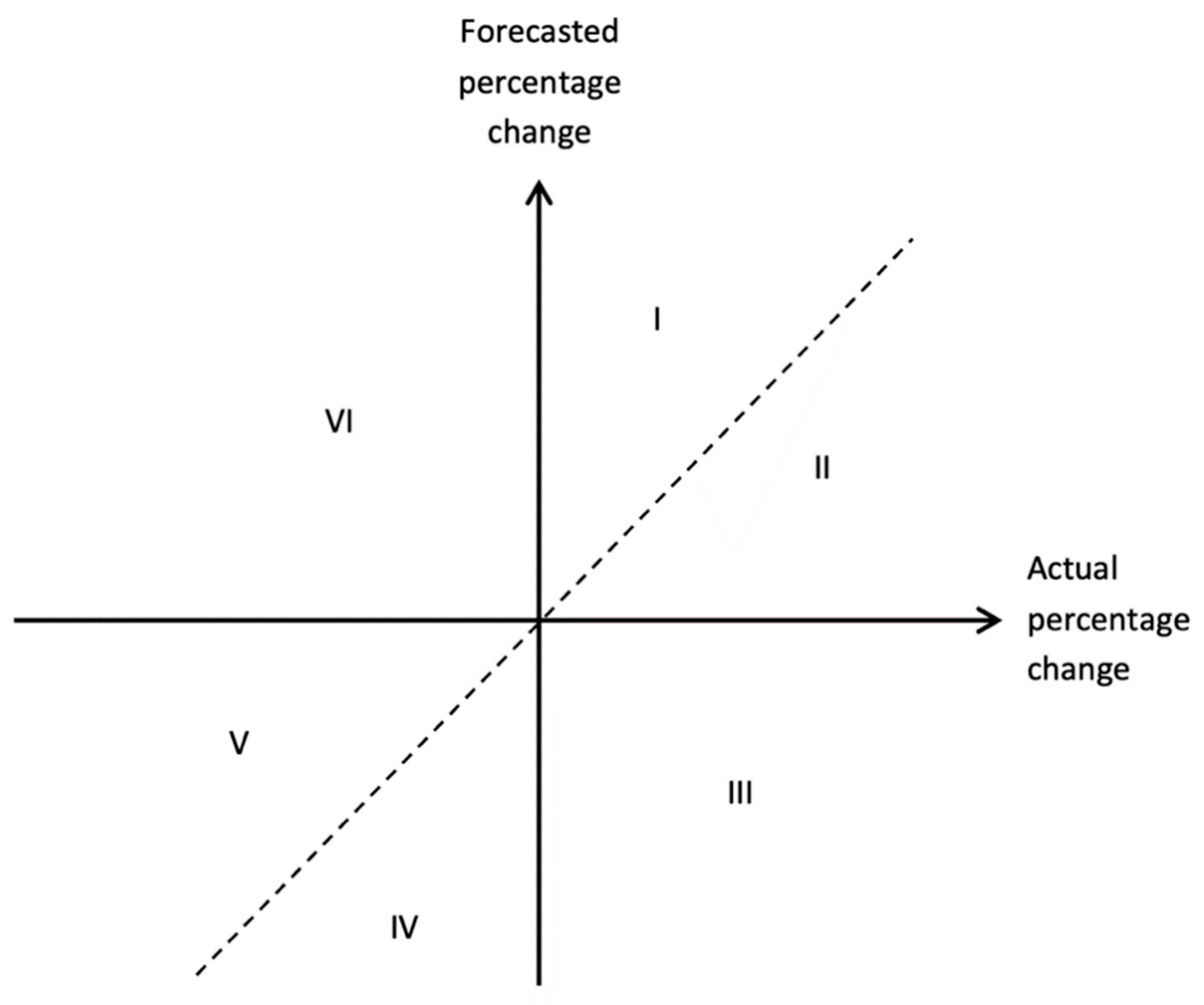
The forecasted percentage changes and the actual percentage changes are plotted and compared in the prediction-realization diagram (Figure 2). The dashed diagonal line in the prediction-realization diagram reflects the area in which the forecasted percentage changes and the actual realized percentage changes coincide (perfect forecasts). A good forecast time series is therefore characterized by the fact that the values are close to the diagonal. Using an OLS regression, we examine whether the slope of the regression line resulting from the forecasts considered is equal to one. When the variability of actual events is systematically underestimated, the slope of the regression lines in the prediction-realization diagram should be lower than one. A flat course of the regression lines (slope < 1) indicates an underestimation of the actual changes.

For all forecasters who have been taking part in forecasting surveys for at least ten years, we determine the slope of the regression lines individually. All of the other forecasts are evaluated within the framework of the total number of forecasts analyzed and within the framework of the consensus forecasts.

Furthermore, we perform the unbiasedness test using the Mincer–Zarnowitz regression (Mincer and Zarnowitz 1969) to examine whether forecasting errors are systematic. The Mincer–Zarnowitz regression takes the following form:

$$A_t=\alpha +\beta P_t+u_t$$

(2)

• $A_t$ = event that actually occurred in time t (dependent variable);
• $\alpha$ = constant;
• $\beta$ = coefficient of the respective forecast;
• $P_t$ = forecast of the actual event in time t;
• $u_t$ = error term in time t.

Based on this equation, forecasts are considered unbiased if α is not significantly different to 0, and β is not significantly different to 1. Likewise, the error term u_t may not be autocorrelated. Forecasts are considered unbiased when, with a low probability of error, the joint hypothesis of α = 0 and β = 1 does not have to be rejected. This is checked by using the Wald test (Wald 1943). A further condition is the absence of autocorrelation in the values of the error term u_t, which is examined with the Wooldridge test (Wooldridge 2002). If, according to these criteria, a forecast time series is unbiased, Granger and Newbold (1974) argue that this by no means signifies that the forecasts are perfect. They merely do not exhibit any systematic errors.

Finally, we compare the forecasts with the naïve forecast. A forecaster who has obtained a notable insight into the future trend of the subject matter should at least be able to make more accurate forecasts than if one were to always assume that nothing at all will change (naïve forecast).

Simple measurements of forecast quality (such as the mean absolute squared error or the mean squared error) enable us to make a comparison with a naïve forecast. However, these simple approaches do not permit an assessment of statistical significance. This deficit is remedied by using the Diebold–Mariano test (Diebold and Mariano 1995). To do so, we calculate the mean squared error for the time series of the expert prognoses and for the time series of the naïve forecasts. The test statistics of the Diebold–Mariano test are defined as follows:

$$DM=\frac{\frac{1}{T}\hspace{0.17em}\sum (V(P_{t\hspace{0.17em}1})\hspace{0.17em}-\hspace{0.17em}V(P_{t2}))}{\sqrt{\widehat{\gamma }\hspace{0.17em}d/T}}$$

(3)

• T = number of observations;
• V = loss function;
• P₁ = naïve forecast;
• P₂ = expert forecast;
• $\sqrt{\widehat{\gamma }\hspace{0.17em}d/T}$ = joint spread of the two loss functions.

The null hypothesis tested in this way is that the naïve forecast (P₁) and the expert forecast (P₂) have the same accuracy. Neither one of the two alternatives thus provides clearly better results. The numerator is the mean deviation between the loss function V of the two forecasting approaches to be compared. Normally a squared loss function is assumed. In other words, the squared errors of the two forecast approaches are compared (P₁ and P₂). The denominator is the joint spread of the two loss functions. This is estimated on the basis of the long-term autocovariances of the loss function. In the case of large samples, this test value is asymptotically normally distributed.

As the methods and variables used by the forecasters in our data basis are not disclosed, we focus on the overall quality of the forecasts in terms of accuracy and unbiasedness. An assessment of the informative value of different forecasting approaches is not in the scope in this study.

5. Results

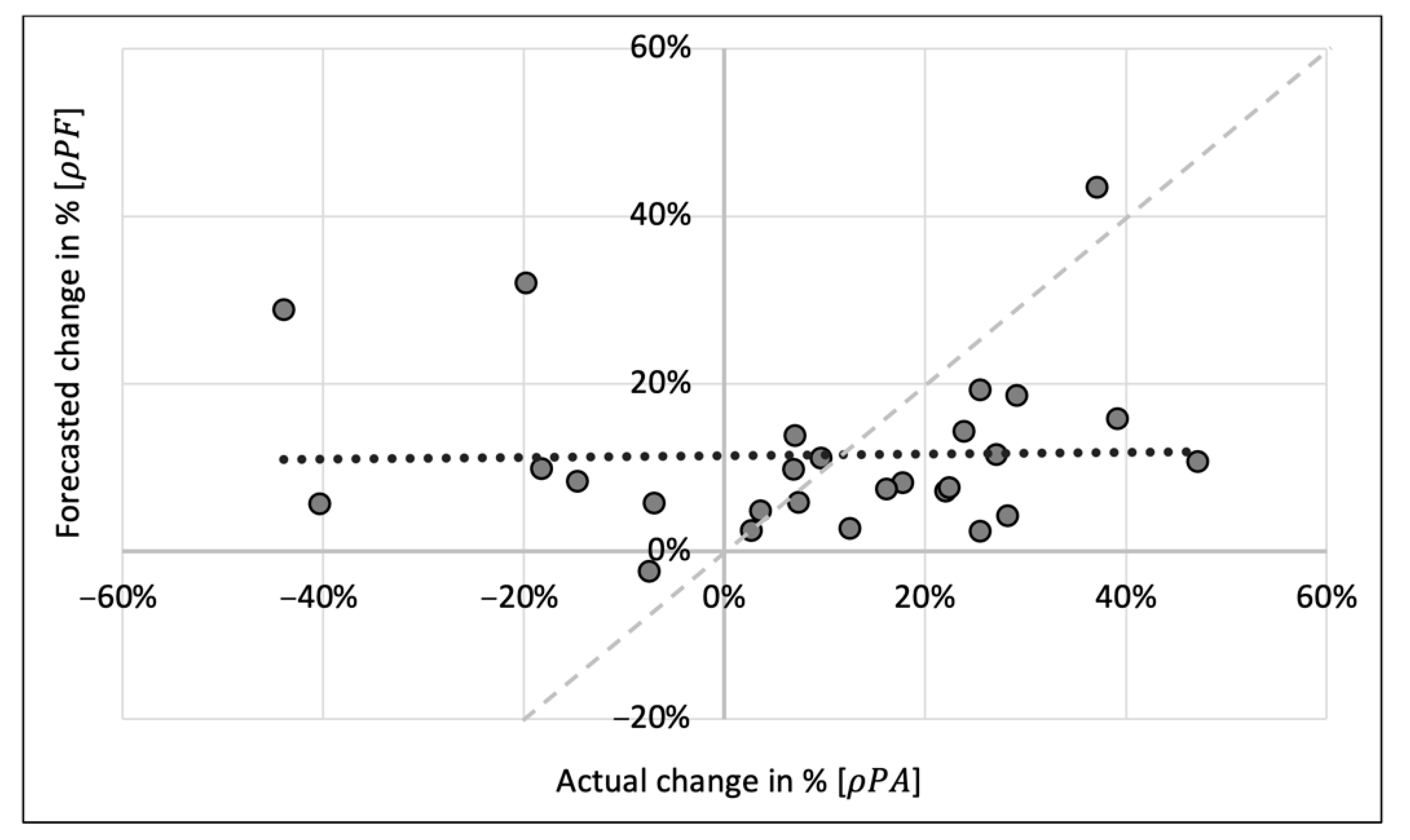
To provide a more detailed insight into our results, we first show the individual forecast quality of two selected German private banks. The graphic representation of the DAX forecasts of the German private bank Berenberg in a prediction-realization diagram indicates that conservative forecasting is at work here (Figure 3).

Berenberg issued a total of 27 DAX forecasts in the observation period (1992–2020). It is recognizable straight away that only one fall in the DAX is forecasted (3rd quadrant), but that the DAX actually does fall in seven out of the 27 years (3rd and 4th quadrant). This means that unusual events (falls in the DAX) are under-represented in the forecasts.

In addition, it can be seen that the dispersion of the actual events (scattering along the $\rho PA$ axis) is greater than the dispersion of the forecasts (scattering along the $\rho PF$ axis). The standard deviation of the actual events is 22.76%. The standard deviation of the forecasts, however, is only 9.98% (

Table 3. The main results of the DAX forecasts from 1992 to 2020 from the Handelsblatt.

Institution	Forecasts Issued	Forecast		Actual		Normal Events over- Represented in the Forecasts	Standard Deviation		SD of the Forecasts < SD of the Actual Events	Regression Line		Slope of the Regression Lines < 1
		DAX Falls	DAX Rises	DAX Falls	DAX Rises		Forecast	Actual		Intercept	Slope
Bank Julius Bär	23	2	21	8	15	Yes	0.062	0.248	Yes	0.088	−0.023	Yes
Bank of America	11	0	11	2	9	Yes	0.066	0.207	Yes	0.117	−0.001	Yes
Bankhaus Lampe	25	1	24	6	19	Yes	0.081	0.234	Yes	0.089	0.097	Yes
Bayerische Landesbank	26	1	25	6	20	Yes	0.067	0.230	Yes	0.080	−0.006	Yes
Berenberg	27	1	26	7	20	Yes	0.100	0.228	Yes	0.114	0.011	Yes
Bethmann Bank	12	2	10	5	7	Yes	0.095	0.284	Yes	0.101	−0.109	Yes
BNP Paribas	18	3	15	4	14	Yes	0.061	0.223	Yes	0.056	0.140	Yes
Commerzbank	28	2	26	7	21	Yes	0.089	0.234	Yes	0.120	−0.064	Yes
Credit Suisse	13	2	11	5	8	Yes	0.072	0.290	Yes	0.106	0.059	Yes
Dekabank	19	1	18	4	15	Yes	0.101	0.227	Yes	0.090	0.154	Yes
Deutsche Bank	25	2	23	7	18	Yes	0.070	0.237	Yes	0.091	−0.043	Yes
Dresdner Bank	15	0	15	5	10	Yes	0.084	0.276	Yes	0.080	0.099	Yes
DZ Bank	29	7	22	8	21	Yes	0.107	0.231	Yes	0.073	0.088	Yes
Haspa	13	0	13	3	10	Yes	0.047	0.202	Yes	0.080	0.045	Yes
Hauck & Aufhäuser	26	5	21	6	20	Yes	0.101	0.235	Yes	0.072	−0.040	Yes
Helaba	28	8	20	7	21	No	0.108	0.234	Yes	0.053	0.092	Yes
HSBC Trinkaus	22	3	19	7	15	Yes	0.085	0.256	Yes	0.080	−0.022	Yes
J.P. Morgan	22	4	18	6	16	Yes	0.100	0.244	Yes	0.084	0.038	Yes
LBB Landesbank Berlin	18	3	15	6	12	Yes	0.140	0.233	Yes	0.088	0.027	Yes
LBBW	21	1	20	6	15	Yes	0.107	0.226	Yes	0.090	0.093	Yes
Lehman Brothers	12	5	7	4	8	No	0.098	0.259	Yes	0.040	0.062	Yes
M.M. Warburg & Co.	29	3	26	8	21	Yes	0.091	0.231	Yes	0.076	−0.016	Yes
Morgan Stanley	14	6	8	4	10	No	0.123	0.285	Yes	0.030	0.136	Yes
National-Bank	15	3	12	3	12	No	0.086	0.202	Yes	0.082	0.028	Yes
NATIXIS	17	1	16	3	14	Yes	0.065	0.231	Yes	0.077	0.057	Yes
NordLB	12	2	10	2	10	No	0.038	0.153	Yes	0.041	−0.089	Yes
Oddo BHF	28	3	25	8	20	Yes	0.104	0.234	Yes	0.090	0.059	Yes
Pictet & Cie.	13	3	10	5	8	Yes	0.114	0.279	Yes	0.092	−0.074	Yes
Postbank	11	0	11	3	8	Yes	0.069	0.225	Yes	0.098	0.087	Yes
Sal. Oppenheim	21	2	19	5	16	Yes	0.093	0.248	Yes	0.067	0.111	Yes
Santander	24	1	23	7	17	Yes	0.093	0.239	Yes	0.116	0.101	Yes
Société Générale	20	4	16	5	15	Yes	0.096	0.228	Yes	0.065	0.043	Yes
SYZ & Co.	10	0	10	2	8	Yes	0.058	0.235	Yes	0.144	−0.042	Yes
UBS	14	3	11	4	10	Yes	0.120	0.242	Yes	0.112	0.007	Yes
Unicredit HypoVereinsbank	28	3	25	8	20	Yes	0.079	0.233	Yes	0.083	0.043	Yes
VP Bank	11	1	10	2	9	Yes	0.042	0.155	Yes	0.084	0.034	Yes
WestLB	21	3	18	7	14	Yes	0.106	0.260	Yes	0.081	0.124	Yes
WGZ Bank	16	1	15	5	11	Yes	0.172	0.211	Yes	0.110	0.301	Yes
Consensus	29	1	28	8	21	Yes	0.065	0.231	Yes	0.085	0.037	Yes
All forecasts	964	117	847	264	700	Yes	0.091	0.230	Yes	0.084	0.034	Yes

DAX = German Stock Market Index; SD = standard deviation.

). The slope in the dotted regression line in the prediction-realization diagram of 0.011 is thus nowhere near the threshold value 1 (dashed diagonal line) (Table 3). The variability of the actual events is dramatically underestimated.

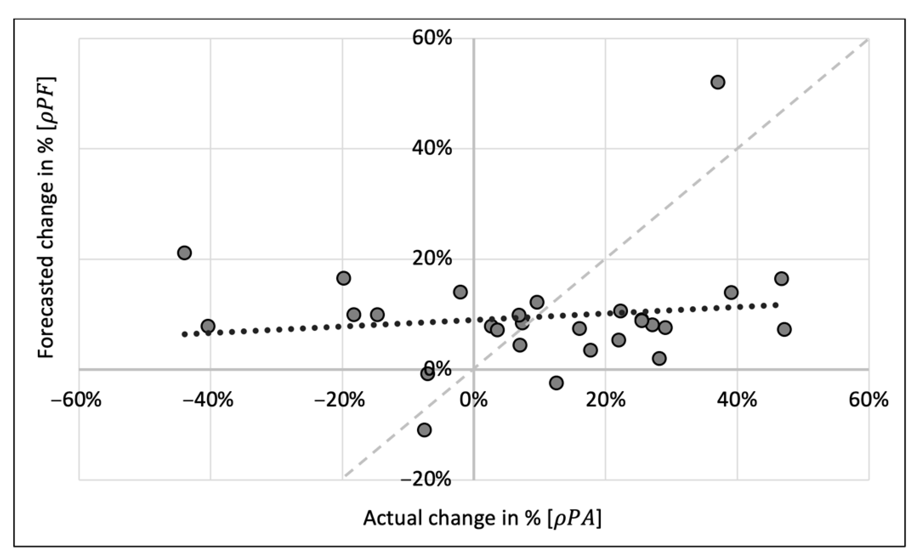
As another example, we consider the prediction-realization diagram of DAX forecasts made by the Franco-German private bank Oddo BHF (Figure 4).

This reveals a picture which is very similar to that of the prediction-realization diagram for Berenberg. In the period 1992–2020, at the end of each year Oddo BHF forecasts the DAX for the coming year. This occurs a total of 28 times. A fall in the DAX is forecasted on three occasions. In reality, however, the DAX falls in eight of the 28 years. This means that unusual events (falls in the DAX) are under-represented in the forecasts.

In addition, it can be seen that the dispersion of the actual events (scattering along the $\rho PA$ axis) is greater than the dispersion of the forecasts (scattering along the $\rho PF$ axis). The standard deviation of the actual events is 23.39%. The standard deviation of the forecasts, however, is only 10.41% (Table 3). The slope of 0.059 in the dotted regression line in the prediction-realization diagram is thus nowhere near the threshold value 1 (dashed diagonal line) (Table 3). The variability of the actual events is dramatically underestimated.

Table 3 depicts the main results of the DAX forecasts from the Handelsblatt newspaper. All of the forecasters who have taken part in the forecasting surveys of the Handelsblatt for at least ten years are analyzed individually. All of the forecasters who issue less than 10 forecasts in the period from 1992 to 2020 are not analyzed individually but are taken into account as part of the overall analysis of all forecasts and within the framework of the consensus forecasts (final lines in Table 3).

The seventh column of Table 3 indicates whether fewer falls in the DAX are forecasted than actually occur. As the DAX is a performance index and exhibits a rising trend over the long term, all falls in the index are interpreted as ‘unusual events’. According to Ogburn (1934), conservative forecasting leads to ‘normal events’ (here: an increase in the DAX) being over-represented in the forecasts, while ‘unusual events’ (here: a decrease in the DAX) are under-represented in the forecasts. This is the case in 33 of the 38 forecasters who are analyzed individually here: a proportion of 86.8%. Unusual events are also under-represented in the consensus forecasts and when the total number of the forecasts is considered as a whole. The detailed data is given in Table 3, where one can see how often a falling DAX was forecast, and how often the DAX really falls. One can also note how often an upward trend was forecast for the DAX, and how often the DAX really rises (Table 3).

The picture is clearer in the case of the standard deviations. According to Ogburn (1934), conservative forecasting leads to standard deviations of the forecasts which are lower than the standard deviations of the actual events. The tenth column of Table 3 considers whether this applies to the DAX forecasts and reveals that this is the case in all 38 of the 38 forecasters analyzed. Also, with regard to the consensus forecasts and when all 964 forecasts are considered, the standard deviation of the forecasts lags behind the standard deviation of the actual events (Table 3).

Ogburn (1934) states that conservative forecasting leads to an underestimation of the variability of reality. In the prediction-realization diagram, this should lead to a slope in the regression lines which is lower than one. The last column of Table 3 illustrates this aspect. It can be seen that in 38 out of 38 cases, the slope in the regression lines is lower than one. The fact that the slopes are usually clearly below the threshold value of one is also revealed in the detailed data on the intercepts and the slopes in the regression lines (Table 3).

The German quality newspaper the Frankfurter Allgemeine Zeitung (FAZ) only started a regular survey of forecasts in 2002. As a result, the share price falls in the years 2000 and 2001 no longer have an effect. It is interesting to see whether this leads to significantly different results in the forecasts. In addition, the Frankfurter Allgemeine Zeitung not only surveys annual forecasts, but also six-month forecasts. It is quite possible that the characteristics of the forecasts with differing forecast horizons vary. Once again, all of the forecasters who have taken part in the forecasting surveys of the FAZ at least ten times are analyzed individually (

Table 4. The main results of the DAX forecasts from 2002 to 2020 from the FAZ.

Institution	Forecasts Issued	Forecast		Actual		Normal Events over- Represented in the Forecasts	Standard Deviation		SD of the Forecasts < SD of the Actual Events	Regression Line		Slope of the Regression Lines < 1
		DAX Falls	DAX Rises	DAX Falls	DAX Rises		Forecast	Actual		Intercept	Slope
Forecast horizon 6 months
Bayern LB	10	5	5	3	7	No	0.047	0.094	Yes	0.028	−0.286	Yes
Deka Bank	16	3	13	5	11	Yes	0.061	0.096	Yes	0.040	−0.002	Yes
DZ Bank	16	6	10	5	11	No	0.065	0.096	Yes	0.009	0.032	Yes
Helaba	14	6	8	5	9	No	0.075	0.102	Yes	0.025	−0.375	Yes
HSH Nordbank	10	7	3	4	6	No	0.095	0.098	Yes	−0.030	−0.039	Yes
HVB-Unicredit Bank	16	4	12	6	10	Yes	0.063	0.104	Yes	0.035	−0.035	Yes
LBBW	17	3	14	6	11	Yes	0.048	0.102	Yes	0.019	0.090	Yes
M.M. Warburg	17	3	14	6	11	Yes	0.122	0.102	No	0.030	−0.039	Yes
Oddo BHF	10	1	9	4	6	Yes	0.041	0.121	Yes	0.049	−0.058	Yes
Postbank	13	6	7	4	9	No	0.071	0.104	Yes	0.008	−0.087	Yes
Santander Asset Mgmt.	13	1	12	3	10	Yes	0.029	0.099	Yes	0.033	0.073	Yes
Société Générale	10	6	4	3	7	No	0.087	0.072	No	−0.023	−0.431	Yes
Consensus	17	2	15	6	11	Yes	0.028	0.102	Yes	0.024	−0.077	Yes
All forecasts	282	83	199	103	179	Yes	0.072	0.095	Yes	0.024	−0.076	Yes
Forecast horizon 12 months
Allianz SE	11	0	11	2	9	Yes	0.044	0.155	Yes	0.072	0.018	Yes
Bayern LB	11	0	11	2	9	Yes	0.036	0.159	Yes	0.069	0.011	Yes
BNP Paribas	12	1	11	3	9	Yes	0.055	0.210	Yes	0.066	0.110	Yes
Commerzbank	18	0	18	4	14	Yes	0.081	0.233	Yes	0.119	0.032	Yes
Deka Bank	18	1	17	3	15	Yes	0.104	0.195	Yes	0.082	0.200	Yes
Deutsche Bank	10	0	10	2	8	Yes	0.047	0.212	Yes	0.104	−0.017	Yes
DWS	13	0	13	3	10	Yes	0.027	0.202	Yes	0.076	0.038	Yes
DZ Bank	18	2	16	4	14	Yes	0.066	0.222	Yes	0.072	0.063	Yes
Helaba	15	6	9	3	12	No	0.121	0.196	Yes	0.025	0.249	Yes
HSBC Trinkaus & Burkhardt	13	2	11	3	10	Yes	0.066	0.262	Yes	0.065	−0.102	Yes
HSH Nordbank	11	2	9	3	8	Yes	0.080	0.213	Yes	0.055	0.192	Yes
HVB-Unicredit Bank	18	1	17	4	14	Yes	0.078	0.228	Yes	0.077	0.077	Yes
J.P. Morgan	12	1	11	3	9	Yes	0.064	0.233	Yes	0.095	0.140	Yes
LBBW	19	0	19	4	15	Yes	0.097	0.227	Yes	0.091	0.093	Yes
M.M. Warburg	19	1	18	4	15	Yes	0.097	0.227	Yes	0.078	−0.018	Yes
Oddo BHF	17	1	16	4	13	Yes	0.045	0.225	Yes	0.093	−0.092	Yes
Postbank	14	0	14	3	11	Yes	0.070	0.208	Yes	0.096	0.048	Yes
Santander Asset Mgmt.	16	0	16	3	13	Yes	0.052	0.195	Yes	0.107	0.048	Yes
Société Générale	11	4	7	2	9	No	0.088	0.155	Yes	0.067	−0.347	Yes
UBS	10	1	9	1	9	No	0.118	0.151	Yes	0.136	0.027	Yes
WestLB	11	2	9	3	8	Yes	0.128	0.282	Yes	0.075	0.204	Yes
Consensus	19	0	19	4	15	Yes	0.061	0.227	Yes	0.087	0.064	Yes
All forecasts	402	31	371	88	314	Yes	0.083	0.215	Yes	0.085	0.054	Yes

DAX = German Stock Market Index; FAZ = Frankfurter Allgemeine Zeitung; SD = standard deviation.

).

The results are in fact somewhat less clear than those for the DAX forecasts from the Handelsblatt. In 24 out of 33 cases (72.7%), normal events (increase in the DAX) are over-represented in the forecasts (seventh column in Table 4). Unusual events are also under-represented in the consensus forecasts and when all 282 six-month and all 402 twelve-month forecasts are considered as a whole.

The result of the standard deviations is quite clear: In 31 out of 33 cases (93.9%), the forecasts lag behind the actual events (tenth column in Table 4). This finding also applies to the consensus forecasts as well as when all 282 six-month and all 402 twelve-month forecasts are considered as a whole.

The fact that the forecasters persistently underestimate the variability of reality is revealed most clearly in the slope of the regression lines in the prediction-realization diagram (last column in Table 4). In 33 out of 33 cases, the slope is below one. This result also applies to the consensus forecasts as well as when all 282 six-month and all 402 twelve-month forecasts are considered as a whole.

The forecasts of the Dow Jones Industrial Index yield only slightly different results. Once again, all of the forecasters who have taken part in the forecasting survey at least ten times are analyzed individually (

Table 5. Main results of the forecasts of the DJI from 2004 to 2020 from the FAZ.

Institution	Forecasts Issued	Forecast		Actual		Normal Events over-Represented in the Forecasts	Standard Deviation		SD of the Forecasts < SD of the Actual Events	Regression Line		Slope of the Regression Lines < 1
		DJI Falls	DJI Rises	DJI Falls	DJI Rises		Forecast	Actual		Intercept	Slope
Forecast horizon 6 months
Deka Bank	15	5	10	8	7	Yes	0.070	0.066	No	0.018	0.171	Yes
Helaba	14	6	8	6	8	No	0.081	0.077	No	0.019	−0.406	Yes
LBBW	16	7	9	8	8	Yes	0.052	0.073	Yes	0.010	0.116	Yes
M.M. Warburg	15	3	12	7	8	Yes	0.061	0.075	Yes	0.034	0.233	Yes
Postbank	12	6	6	5	7	No	0.053	0.079	Yes	0.003	0.035	Yes
Santander Asset Mgmt.	13	1	12	6	7	Yes	0.019	0.081	Yes	0.026	−0.095	Yes
Consensus	16	4	12	8	8	Yes	0.019	0.073	Yes	0.014	0.036	Yes
All forecasts	203	67	136	106	97	Yes	0.061	0.070	Yes	0.014	0.040	Yes
Forecast horizon 12 months
BNP Paribas	10	0	10	3	7	Yes	0.040	0.183	Yes	0.072	−0.059	Yes
Commerzbank	10	0	10	3	7	Yes	0.052	0.169	Yes	0.081	0.120	Yes
Deka Bank	16	6	10	4	12	No	0.099	0.137	Yes	0.051	0.002	Yes
Helaba	15	7	8	3	12	No	0.107	0.149	Yes	0.008	0.193	Yes
HSH Nordbank	11	5	6	3	8	No	0.067	0.163	Yes	0.022	−0.032	Yes
LBBW	17	4	13	4	13	No	0.058	0.142	Yes	0.053	−0.042	Yes
M.M. Warburg	17	1	16	4	13	Yes	0.071	0.142	Yes	0.063	−0.107	Yes
Oddo BHF	15	0	15	3	12	Yes	0.022	0.147	Yes	0.058	0.054	Yes
Postbank	13	0	13	3	10	Yes	0.063	0.160	Yes	0.084	0.012	Yes
Santander Asset Mgmt.	16	0	16	4	12	Yes	0.051	0.146	Yes	0.070	0.093	Yes
Consensus	17	0	17	4	13	Yes	0.033	0.142	Yes	0.055	0.006	Yes
All forecasts	259	33	226	65	194	Yes	0.066	0.140	Yes	0.057	0.029	Yes

DJI = Dow Jones Industrial Index; FAZ = Frankfurter Allgemeine Zeitung; SD = standard deviation.

).

The Dow Jones Industrial Index is a price index, but it exhibits a long-term rising trend, nevertheless. To this extent, one can also presume here that a rise in the index can be considered a normal event, and that a fall in the index represents an unusual event. In ten out of 16 cases (62.5%), normal events (increase of the Dow Jones Industrial Index) are over-represented in the forecasts (seventh column in Table 5). Unusual events are also under-represented in the consensus forecasts and when all 203 six-month and all 259 twelve-month forecasts are considered as a whole.

The result for the standard deviations is more marked. In 14 out of 16 cases (87.5%), the fluctuations in the forecasts lag behind those of the actual events (tenth column in Table 5). This finding also applies to the consensus forecasts as well as when all 203 six-month and all 259 twelve-month forecasts are considered as a whole.

The fact that the forecasters persistently underestimate the variability of reality is revealed most clearly in the slope of the regression lines in the prediction-realization diagram (last column in Table 5). In 16 out of 16 cases, the slope is below one. This is also the same for the consensus forecasts as well as when all 203 six-month and all 259 twelve-month forecasts are viewed as a whole.

The picture drawn by the forecasts of the Euro Stoxx 50 is even more distinct (

Table 6. The main results for the Euro Stoxx 50 forecasts from 2002 to 2020 from the FAZ.

Institution	Forecasts Issued	Forecast		Actual		Normal Events over-Represented in the Forecasts	Standard Deviation		SD of the Forecasts < SD of the Actual Events	Regression Line		Slope of the Regression Lines < 1
		SX5E Falls	SX5E Rises	SX5E Falls	SX5E Rises		Forecast	Actual		Intercept	Slope
Forecast horizon 6 months
Bayern LB	10	4	6	5	5	Yes	0.043	0.078	Yes	0.011	−0.244	Yes
Deka Bank	16	3	13	8	8	Yes	0.063	0.093	Yes	0.049	0.022	Yes
DZ Bank	16	3	13	8	8	Yes	0.064	0.093	Yes	0.030	0.186	Yes
Helaba	14	6	8	8	6	Yes	0.079	0.095	Yes	0.019	−0.406	Yes
HSH Nordbank	10	6	4	6	4	No	0.085	0.099	Yes	−0.030	−0.214	Yes
HVB-Unicredit Bank	16	3	13	8	8	Yes	0.070	0.101	Yes	0.023	−0.085	Yes
LBBW	17	6	11	9	8	Yes	0.053	0.098	Yes	0.028	0.088	Yes
M.M. Warburg	16	2	14	8	8	Yes	0.073	0.101	Yes	0.055	−0.014	Yes
Oddo BHF	10	2	8	5	5	Yes	0.042	0.116	Yes	0.033	−0.009	Yes
Postbank	13	6	7	7	6	Yes	0.060	0.097	Yes	0.004	−0.100	Yes
Santander Asset Mgmt.	13	2	11	6	7	Yes	0.033	0.099	Yes	0.030	0.110	Yes
Consensus	17	5	12	9	8	Yes	0.030	0.098	Yes	0.023	−0.018	Yes
All forecasts	270	82	188	144	126	Yes	0.073	0.094	Yes	0.023	−0.007	Yes
Forecast horizon 12 months
Allianz SE	11	0	11	4	7	Yes	0.042	0.130	Yes	0.071	−0.035	Yes
Bayern LB	11	0	11	3	8	Yes	0.039	0.127	Yes	0.058	−0.044	Yes
BNP Paribas	11	1	10	3	8	Yes	0.044	0.194	Yes	0.076	−0.069	Yes
Commerzbank	18	1	17	5	13	Yes	0.064	0.195	Yes	0.080	0.017	Yes
Deka Bank	18	1	17	5	13	Yes	0.093	0.170	Yes	0.094	0.107	Yes
DWS	12	0	12	5	7	Yes	0.043	0.175	Yes	0.078	−0.019	Yes
DZ Bank	18	1	17	6	12	Yes	0.075	0.193	Yes	0.090	0.096	Yes
Helaba	15	5	10	5	10	No	0.117	0.177	Yes	0.048	0.292	Yes
HSBC Trinkaus&Burkhardt	14	3	11	4	10	Yes	0.082	0.209	Yes	0.065	−0.141	Yes
HSH Nordbank	11	1	10	4	7	Yes	0.071	0.195	Yes	0.076	0.119	Yes
HVB-Unicredit Bank	18	0	18	6	12	Yes	0.064	0.193	Yes	0.070	0.050	Yes
LBBW	19	1	18	6	13	Yes	0.078	0.190	Yes	0.088	0.003	Yes
M.M. Warburg	19	1	18	6	13	Yes	0.083	0.190	Yes	0.074	−0.073	Yes
Oddo BHF	17	1	16	6	11	Yes	0.047	0.192	Yes	0.072	−0.074	Yes
Postbank	14	0	14	4	10	Yes	0.054	0.190	Yes	0.086	0.032	Yes
Santander Asset Mgmt.	16	0	16	5	11	Yes	0.053	0.178	Yes	0.095	0.078	Yes
WestLB	11	1	10	4	7	Yes	0.088	0.231	Yes	0.073	0.127	Yes
Consensus	19	0	19	6	13	Yes	0.044	0.190	Yes	0.083	0.020	Yes
All forecasts	381	29	352	123	258	Yes	0.073	0.179	Yes	0.080	0.017	Yes

SX5E = Euro Stoxx 50; FAZ = Frankfurter Allgemeine Zeitung; SD = standard deviation.

). Here again, all of the forecasters who have taken part in the forecasting survey at least ten times are analyzed individually. All of the other forecasts form part of the consensus forecasts and are also evaluated as part of the total number of forecasts.

Conservatism among forecasters can lead to them forecasting unusual events too rarely. The Euro Stoxx 50 is a price index, but in spite of this it exhibits a long-term upward trend. To this extent, one can also presume here that a rise in the index can be considered a normal event, and that a fall in the index represents an unusual event. In the predictions of 24 of the 26 forecasters analyzed individually (92.3%), unusual events are under-represented (seventh column in Table 6). The consensus forecasts and the overall total of all 270 six-month forecasts and all 381 twelve-month forecasts also show that unusual events are forecast more seldom than they occur in reality.

The standard deviations provide a very clear picture. The standard deviations of the forecasts lag behind the standard deviations of the actual results in 26 out of 26 cases (tenth column in Table 6). This also applies to the consensus forecasts and the overall total of 270 forecasts with a forecast horizon of six months and all 381 forecasts with a forecast horizon of twelve months.

Finally, it can be seen that the slope in the regression lines in the prediction-realization diagrams is significantly below one in 26 out of 26 cases. The forecasters are thus obviously underestimating the variability of reality (last column in Table 6). These findings are also confirmed when the consensus forecasts and the overall total number of forecasts are considered.

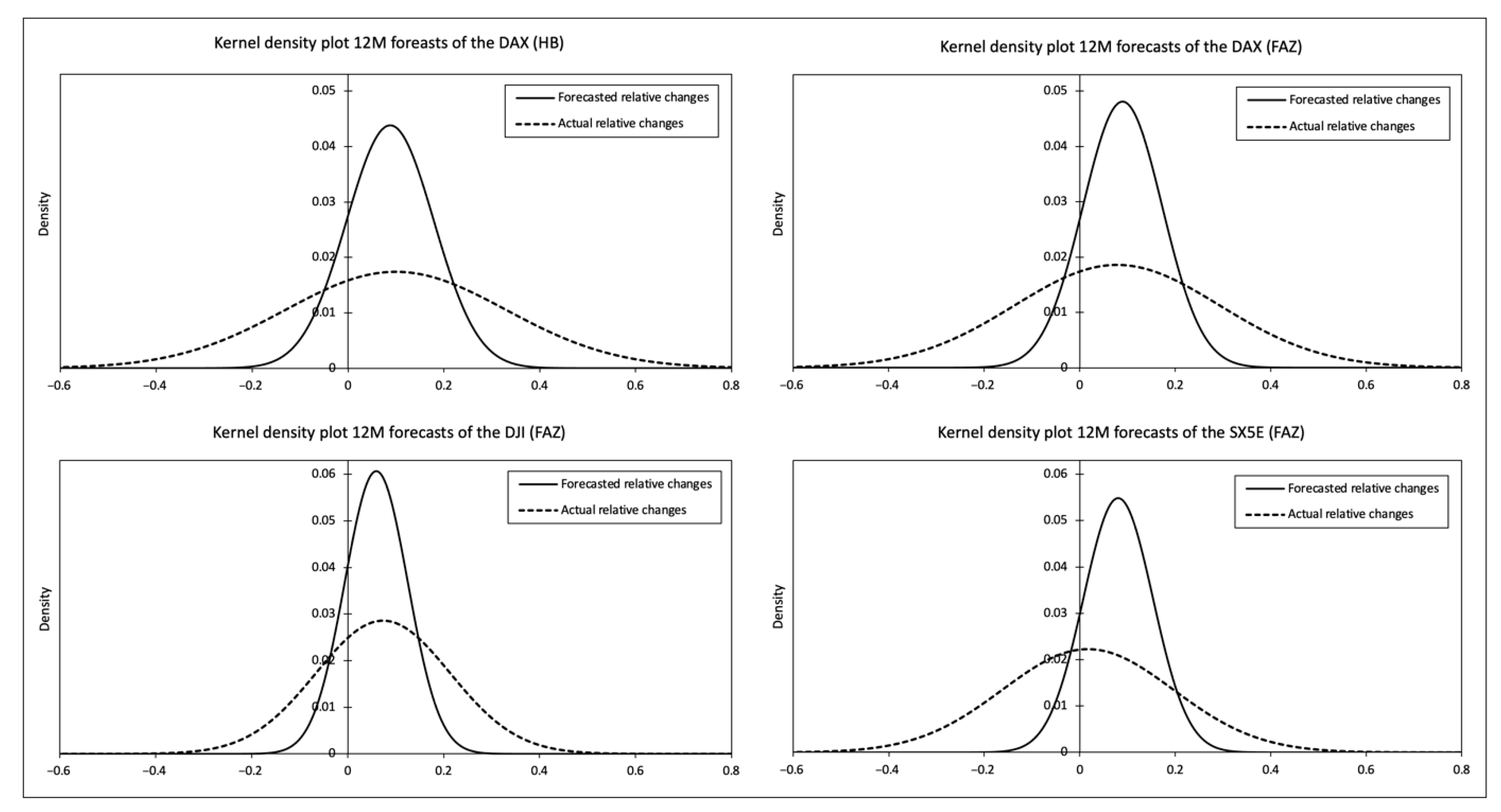
Without exception, it can be observed that the forecasters underestimate the variability of reality. This fact can be clearly seen when looking at the kernel density plots of the forecast relative changes in share prices and the actual relative changes in share prices (Figure 5). The spread of the forecasts is much smaller than the spread of the actual events.

This can be also seen in the fact that the slope in the regression lines in the prediction-realization diagram always remains below the threshold value of one. This leads us to the assessment that this aspect in particular deserves special attention. The unbiasedness test takes the slope of the regression line in the prediction-realization diagram into account as an essential element. Forecasts are viewed as unbiased when the slope in the regression line does not diverge significantly from one, the intercept of the regression line does not deviate significantly from zero, and the residuals are randomly distributed. The decisive advantage of this approach lies in the opportunity to go beyond purely descriptive statistics and to examine the statistical significance of the results.

In all seven cases, it can be seen that given an error probability of ≤1% either the slope of the regression line in the prediction-realization diagram is ≠1 and/or the intercept is ≠ 0. In addition, the residuals are obviously not randomly distributed in six of the seven cases. The forecasts are clearly not unbiased (

Table 7. Unbiasedness test.

Stock Market Index	Source	Forecast Horizon	Number of Observations	Slope	Intercept	F Test p-Value	Wooldridge Test p-Value
DAX	HB	12M	964	0.034	0.084	0.000	0.000
DAX	FAZ	6M	282	−0.075	0.024	0.000	0.000
DAX	FAZ	12M	402	0.054	0.085	0.000	0.006
DJI	FAZ	6M	203	0.040	0.014	0.010	0.098
DJI	FAZ	12M	259	0.029	0.057	0.000	0.623
SX5E	FAZ	6M	270	−0.007	0.023	0.000	0.091
SX5E	FAZ	12M	381	0.017	0.080	0.000	0.042

DAX = German Stock Market Index; DJI = Dow Jones Industrial Index; SX5E = Euro Stoxx 50; HB = Handelsblatt; FAZ = Frankfurter Allgemeine Zeitung; 12M = 12 months; 6M = 6 months.

).

Finally, with the aid of the Diebold–Mariano test we examine whether the quality of the forecasts is significantly superior—from a statistical perspective—to that of naïve forecasts (

Table 8. Comparison of the forecasts with the naïve forecast.

Stock Market Index	Source	Forecast Horizon	Diebold–Mariano Test
			Result	p-Value
DAX	HB	12M	o	0.8143
DAX	FAZ	6M	o	0.1221
DAX	FAZ	12M	o	0.7429
DJI	FAZ	6M	o	0.7053
DJI	FAZ	12M	o	0.3491
SX5E	FAZ	6M	−	0.0000
SX5E	FAZ	12M	−	0.0540

o = no significant result, − = significantly poorer than the naïve forecasts, + = significantly better than the naïve forecast, DAX = German Stock Market Index; DJI = Dow Jones Industrial Index; SX5E = Euro Stoxx 50; HB = Handelsblatt; FAZ = Frankfurter Allgemeine Zeitung; 12M = 12 months; 6M = 6 months.

). The result is that the forecasts of the Euro Stoxx 50 are significantly poorer than the corresponding naïve forecasts, and the quality of the forecasts for the DAX and the Dow Jones Industrial Index does not go significantly beyond that of naïve forecasts.

In

Table 9. The results of hypothesis testing.

Stock Market Index	Source	Forecast Horizon	Hypothesis 1	Hypothesis 2	Hypothesis 3	Hypothesis 4	Hypothesis 5
DAX	HB	12M	+	+	+	+	+
DAX	FAZ	6M	+	+	+	+	+
DAX	FAZ	12M	+	+	+	+	+
DJI	FAZ	6M	+	+	+	+	+
DJI	FAZ	12M	+	+	+	+	+
SX5E	FAZ	6M	+	+	+	+	+
SX5E	FAZ	12M	+	+	+	+	+

+ = Null Hypothesis rejected; DAX = German Stock Market Index; DJI = Dow Jones Industrial Index; SX5E = Euro Stoxx 50; HB = Handelsblatt; FAZ = Frankfurter Allgemeine Zeitung; 12M = 12 months; 6M = 6 months.

the results of the hypothesis testing are summarized. In Hypotheses 1–3, the result which was determined for “all forecasts” in a forecasting area is used. In the case of the DAX forecasts from the Handelsblatt survey, for example, that is the 964 forecasts which are noted in the final line of Table 3. For Hypothesis 4, the results of the unbiasedness test (Table 7) are taken into account, and for Hypothesis 5 the results of the Diebold–Mariano test (Table 8).

In the case of Hypothesis 1 there is a uniform pattern for all areas of forecasting and all forecast horizons. Normal events (index rises) are over-represented in the forecasts. Unusual events (index falls) are under-represented in the forecasts. Null Hypothesis 1 has to be rejected in all seven cases.

In the case of Hypothesis 2 there are no differences between the subjects of the forecasts and the forecast horizons. In all seven cases, Null Hypothesis 2 has to be rejected. The dispersion of the forecasts (measured against the standard deviation) thus lags behind the dispersion of the actual events.

A uniform picture is also shown with regard to Hypothesis 3. In all seven forecasting areas the slope of the regression line in the prediction-realization diagrams is clearly below one. Null Hypothesis 3 has to be rejected in all seven cases. This means that the rates of change of the stock-market indices are significantly underestimated.

In the case of Hypothesis 4 there are also no relevant differences regarding the subjects of the forecasts or the forecast horizons. In all seven areas, the forecasts prove to be biased. These results are highly significant. In all seven cases, Null Hypothesis 4 has to be rejected.

In Hypothesis 5 there is also a concurring result for all seven forecast groups. Null Hypothesis 5 has to be discarded. The precision of the forecasts does not go significantly beyond that of naïve forecasts.

The findings of Ogburn (1934) are thus fully confirmed in the stock market forecasts which we analyzed. It can certainly be stated that these stock-market analysts systematically underestimate the variability of reality and that the success rate of their forecasts does not extend beyond that of naïve forecasts. Their behavior can be described as “sticky” because their forecasts adhere too strongly to long-term trends in the indices to provide meaningful information about current events.

This study expands on existing research as it is the first of its kind to analyze ex-ante forecasts for the SX5E. The picture obtained is similar to that of the stock indices examined previously. The forecasts are mostly biased and not significantly better than naïve forecasts. About 15 years ago, ex-ante forecasts for the DAX and the DJI were last examined (Table 1). In the meantime, technological progress has led to the emergence of numerous promising new forecasting methods, as discussed in our literature review. However, our results indicate that this has not, at least so far, contributed to a significant increase in the quality of the forecast.

Our findings allow different conclusions to be drawn with regard to the efficient market hypothesis (Fama 1970). On the one hand, the Diebold–Mariano test shows that the forecast quality is poor. This is compatible with the efficient market hypothesis, since no excess returns can be achieved on the basis of the forecasts. On the other hand, the efficient market hypothesis assumes that economic subjects are fully informed. The permanent underestimation of the variability of reality that the prediction-realization diagram reveals should therefore not occur. The acting subjects do not seem to take notice of the discrepancy between their own actions and reality, since no correction of the behavior is made in the subsequent forecasts.

The forecasters systematically underestimate the variability of reality. Against the background of Mandelbrot’s fractal theory, it seems reasonable to conclude that forecasters—as long as they think in terms of “trending” and “mean reversion”—systematically underestimate the Hurst exponent (Mandelbrot 2004) of stock market developments.

Overall, the forecast quality for all three indices is not sufficient to enable an active investment strategy on the basis of the forecasts that is likely to be successful. Moreover, since unusual events (e.g., a sudden drop in an otherwise rising trendline) are seldom successfully forecasted, an active investment strategy based on the forecasts harbors risks that can cause severe financial damage to investors. Thus, we advise private and professional investors to consider a passive investment strategy instead when deciding how to invest their assets.

The path which has to be followed to obtain better stock market forecasts thus becomes clear: analysts have to be more courageous. They need to react to new trends with more flexibility. They have to leave their comfort zone more frequently and stand by assessments which are not necessarily approved of by the majority of their peers. That alone will presumably not suffice to generate reliable stock market forecasts: they will also need to work hard on the quality of their approaches to forecasting. To this end, a variety of interesting approaches are already discussed in the literature, e.g., economic forecasts based on newspaper texts or news from online media and attention to news events (Milas et al. 2021; Kalamara et al. 2020; Ben-Rephael et al. 2017). If analysts want to significantly improve the reliability of their forecasts, there is no alternative but to change their overly cautious, highly conservative, and thus inflexible attitudes.

Finally, our study also has some limitations. First of all, it should be mentioned that we are looking at forecasts for entire stock indices. Even if the forecasters do not manage to successfully predict the development of a stock index, this does not mean that the entire stock market is per se unsuitable for an active investment strategy. It is still conceivable that stocks of individual companies in the index can be predicted successfully. In this case, an active investment strategy based on the forecasts for individual stocks could be very promising. Second, forecasting future events with a six- to twelve-month horizon is a major hurdle. As the forecast quality tends to increase as the horizon decreases (Dua 1988), it is conceivable that, for example, monthly forecasts for the same indices would lead to significantly better results. Last but not least, we analyze the entire time series from beginning to end for each forecaster. Even though this leads to a large sample size, which enables a clearer picture of the forecast quality overall, differences in the forecast quality over time may remain undetected. This could be the case in particular for the forecasts published in Handelsblatt, which extend over a period of 29 years.

Our results provide initial indications that patterns discovered almost 90 years ago that massively deteriorate forecast quality can still be found in stock market forecasts today. We therefore encourage future research efforts to examine whether our results prevail in additional datasets. Furthermore, we believe that deeper analysis of the rationale for conservative forecasting and an assessment of its financial impact on investors are promising areas of research that would deepen our understanding of ex-ante stock market forecasts.

6. Summary

We examine forecasts for the German Stock Market Index (DAX), the Dow Jones Industrial Index (DJI), and the Euro Stoxx 50 (SX5E) which were published in the period 1992 to 2020 in the German business newspaper Handelsblatt (HB) and the quality broadsheet the Frankfurter Allgemeine Zeitung (FAZ). These forecasts have a horizon of six and twelve months. The forecasts are from German and international banks such as Deutsche Bank, Goldman Sachs, J.P. Morgan, or BNP Paribas.

We take up the thoughts of Ogburn (1934), who, on the basis of a small empirical survey, became convinced that forecasters consistently underestimate the variability of the future, and that their forecasting is of a conservative nature. However, we also go beyond this and use some contemporary measures (prediction-realization diagram, test of unbiasedness, Diebold–Mariano test) to test ex-ante forecasts for their success at the time of validity.

Conservative forecasting behavior leads to unusual events being under-represented in forecasts, to the dispersion of the forecasts (as measured by their standard deviation) lagging behind the dispersion of the actual events, and to the extent of the forecasted changes being smaller than the actual changes. The latter aspect is reflected in a flat course of the regression line in the prediction-realization diagram (slope < 1) and thus also leads to failure in the unbiasedness test.

We analyze a total of 2,761 forecasts which are divided up into seven groups according to the subject of the forecast (DAX, DJI, SX5E), the forecast horizon (6 and 12 months), and the source (FAZ, HB). The findings are that in all seven groups (a) unusual events are under-represented in the forecasts, (b) the dispersion of the forecasts lags behind that of actual events, (c) the slope in the regression lines in the prediction-realization diagram is <1, (d) the forecasts are biased to a highly significant degree, and (e) that the quality of the forecasts is not significantly better than that of naïve forecasts.

It is more than surprising how closely these stock market forecasts for the years 1992 to 2020 correspond to the characteristics which Ogburn described back in the 1930s. The stock market analysts prove to be too conservative, inflexible, and cautious. If they want to improve the reliability of their forecasts, they should change their conservative and inflexible forecasting behavior and consider promising new approaches and technologies in their forecasting process. For private and professional investors, building active investment strategies based on the insufficient stock market forecasts examined can involve enormous financial risks and is therefore not recommended.

References

- Andres, Peter, and Markus Spiwoks. 1999. Forecast Quality Matrix: A Methodological Survey of Judging Forecast Quality of Capital Market Forecasts. Journal of Economics and Statistics 219: 513–42. [Google Scholar]
- Arthur, W. Brian, John H. Holland, Blake LeBaron, Richard Palmer, and Paul Tayler. 1997. Asset pricing under endogenous expectations in an artificial stock market. In The Economy as an Evolving Complex System II. Edited by W. Brian Arthur, Steven N. Durlauf and David A. Lane. Reading: Addison-Wesley. [Google Scholar]
- Atmaz, Adem, Stefano Cassella, Huseyin Gulen, and Fangcheng Ruan. 2021. Contrarians, Extrapolators, and Stock Market Momentum and Reversal. Available online: https://0-dx-doi-org.brum.beds.ac.uk/10.2139/ssrn.3722540 (accessed on 28 November 2021).
- Atsalakis, George S., and Kimon P. Valavanis. 2009. Forecasting stock market short-term trends using a neuro-fuzzy based methodology. Expert systems with Applications 36: 10696–707. [Google Scholar] [CrossRef]
- Bacchetta, Philippe, Elmar Mertens, and Eric Van Wincoop. 2009. Predictability in financial markets: What do survey expectations tell us? Journal of International Money and Finance 28: 406–26. [Google Scholar] [CrossRef] [Green Version]
- Baghestani, Hamid, Mohammad Arzaghi, and Ilker Kaya. 2015. On the Accuracy of Blue Chip Forecasts of Interest Rates and Country Risk Premiums. Applied Economics 47: 113–22. [Google Scholar] [CrossRef]
- Bahrami, Afsaneh, Abul Shamsuddin, and Katherine Uylangco. 2018. Out-of-sample stock return predictability in emerging markets. Accounting & Finance 58: 727–50. [Google Scholar]
- Ben-Rephael, Azi, Zhi Da, and Ryan D. Israelsen. 2017. It Depends on Where You Search: Institutional Investor Attention and Underreaction to News. Review of Financial Studies 30: 3009–47. [Google Scholar] [CrossRef]
- Benke, Holger. 2006. Was leisten Kapitalmarktprognosen?, Die Sicht eines Stiftungsmanagers. Zeitschrift für das Gesamte Kreditwesen 59: 902–6. [Google Scholar]
- Bertella, Mario A., Felipe R. Pires, Ling Feng, and Harry Eugene Stanley. 2014. Confidence and the Stock Market: An Agent-Based Approach. PLoS ONE 9: e83488. [Google Scholar] [CrossRef] [Green Version]
- Cassella, Stefano, and Huseyin Gulen. 2019. Belief-based Equity Market Sentiment. Available online: https://0-dx-doi-org.brum.beds.ac.uk/10.2139/ssrn.3123083 (accessed on 28 November 2021).
- Cassella, Stefano, and Huseyin Gulen. 2018. Extrapolation Bias and the Predictability of Stock Returns by Price-Scaled Variables. The Review of Financial Studies 31: 4345–97. [Google Scholar] [CrossRef]
- Chen, Shu-Heng, and Ya-Chi Huang. 2008. Risk preference, forecasting accuracy and survival dynamics: Simulations based on a multi-asset agent-based artificial stock market. Journal of Economic Behavior & Organization 67: 702–17. [Google Scholar]
- Chen, Yi-ting, and Kendro Vincent. 2016. The Role of Momentum, Sentiment, and Economic Fundamentals in Forecasting Bear Stock Market. Journal of Forecasting 35: 504–27. [Google Scholar] [CrossRef]
- Cowles, Alfred. 1933. Can stock market forecasters forecast? Econometrica: Journal of the Econometric Society 1: 309–24. [Google Scholar] [CrossRef] [Green Version]
- De Bondt, Werner P. 1993. Betting on trends: Intuitive forecasts of financial risk and return. International Journal of Forecasting 9: 355–71. [Google Scholar] [CrossRef]
- Diebold, Francis X., and Robert S. Mariano. 1995. Comparing Predictive Accuracy. Journal of Business and Economic Statistics 13: 253–63. [Google Scholar]
- Dimson, Elroy, and Paul Marsh. 1984. An analysis of brokers’ and analysts’ unpublished forecasts of UK stock returns. The Journal of Finance 39: 1257–92. [Google Scholar] [CrossRef]
- Dua, Pami. 1988. Multiperiod forecasts of interest rates. Journal of Business & Economic Statistics 6: 381–84. [Google Scholar]
- Fama, Eugene. 1970. Efficient Capital Markets: A Review of Theory and Empirical Work. The Journal of Finance 25: 383–417. [Google Scholar] [CrossRef]
- Fassas, Athanasios, Stephanos Papadamou, and Dimitrios Kenourgios. 2021. Evaluating survey-based forecasts of interest rates and macroeconomic variables. Journal of Economic Studies. [Google Scholar] [CrossRef]
- Filiz, Ibrahim, Jan René Judek, Marco Lorenz, and Markus Spiwoks. 2021. Interest rate forecasts in Latin America. Journal of Economic Studies. [Google Scholar] [CrossRef]
- Filiz, Ibrahim, Thomas Nahmer, Markus Spiwoks, and Kilian Bizer. 2019. The accuracy of interest rate forecasts in the Asia-Pacific region: Opportunities for portfolio management. Applied Economics 51: 6309–32. [Google Scholar] [CrossRef]
- Fraser, Patricia, and Ronald MacDonald. 1993. The efficiency of CAC stock price forecasts: A survey based perspective. Revue Économique 44: 991–1000. [Google Scholar]
- Friend, Irwin, and Douglas Vickers. 1965. Portfolio selection and investment performance. The Journal of Finance 20: 391–415. [Google Scholar] [CrossRef]
- Fujiwara, Ippei, Hibiki Ichiue, Yoshiyuki Nakazono, and Yosuke Shigemi. 2013. Financial markets forecasts revisited: Are they rational, stubborn or jumpy? Economics Letters 118: 526–30. [Google Scholar] [CrossRef]
- Goyal, Amit, Ivo Welch, and Athanasse Zafirov. 2021. A Comprehensive Look at the Empirical Performance of Equity Premium Prediction II. Available online: https://0-dx-doi-org.brum.beds.ac.uk/10.2139/ssrn.3929119 (accessed on 28 November 2021).
- Granger, Clive W., and Paul Newbold. 1974. Spurious regressions in econometrics. Journal of Econometrics 2: 111–20. [Google Scholar] [CrossRef] [Green Version]
- Greenwood, Robin, and Andrei Shleifer. 2014. Expectations of Returns and Expected Returns. The Review of Financial Studies 27: 714–46. [Google Scholar] [CrossRef] [Green Version]
- Guo, Hui. 2006. On the out-of-sample predictability of stock market returns. The Journal of Business 79: 645–70. [Google Scholar] [CrossRef]
- Hein, Oliver, Michael Schwind, and Markus Spiwoks. 2012. Network Centrality and Stock Market Volatility: The Impact of Communication Topologies on Prices. Journal of Finance and Investment Analysis 1: 199–232. [Google Scholar]
- Kalamara, Eleni, Arthur Turrell, Chris Redl, George Kapetanios, and Sujit Kapadia. 2020. Making Text Count: Economic Forecasting Using Newspaper Text. Bank of England Research Paper Series 865: 1–49. [Google Scholar] [CrossRef]
- Kandasamy, Narayanan, Sarah N. Garfinkel, Lionel Page, Ben Hardy, Hugo D. Critchley, Mark Gurnell, and John M. Coates. 2016. Interoceptive Ability Predicts Survival on a London Trading Floor. Scientific Reports 6: 32986. [Google Scholar] [CrossRef]
- Kazak, Ekaterina, and Winfried Pohlmeier. 2019. Testing out-of-sample portfolio performance. International Journal of Forecasting 35: 540–54. [Google Scholar] [CrossRef] [Green Version]
- Krichene, Hazem, and Mhamed-Ali El-Aroui. 2018. Artificial stock markets with different maturity levels: Simulation of information asymmetry and herd behavior using agent-based and network models. Journal of Economic Interaction and Coordination 13: 511–35. [Google Scholar] [CrossRef]
- Kunze, Frederik, Markus Spiwoks, Kilian Bizer, and Torsten Windels. 2018. The usefulness of oil price forecasts—Evidence from survey prediction. Managerial and Decision Economics 39: 427–46. [Google Scholar] [CrossRef]
- Kunze, Frederik, Christoph Wegener, Kilian Bizer, and Markus Spiwoks. 2017. Forecasting European interest rates in times of financial crisis—What insights do we get from international survey forecasts? Journal of International Financial Markets, Institutions and Money 48: 192–205. [Google Scholar] [CrossRef]
- Lakonishok, Josef. 1980. Stock market return expectations: Some general properties. The Journal of Finance 35: 921–31. [Google Scholar] [CrossRef]
- Lofthouse, Stephen. 1996. Why Active Investment Management is Popular: The Psychology of Extraordinary Beliefs. Journal of Interdisciplinary Economics 7: 41–61. [Google Scholar] [CrossRef]
- Mallikarjuna, Mejari, and R. Prabhakara Rao. 2019. Evaluation of forecasting methods from selected stock market returns. Financial Innovation 5: 1–16. [Google Scholar] [CrossRef] [Green Version]
- Mandelbrot, Benoit. 2004. The (Mis)Behavior of Markets—A Fractal View of Risk, Ruin and Reward. New York: Basic Books, pp. 186–95. [Google Scholar]
- Maxwell, Michael, and Gary van Vuuren. 2019. Active investment strategies under tracking error constraints. International Advances in Economic Research 25: 309–22. [Google Scholar] [CrossRef]
- Miah, Fazlul, Ahmed Ali Khalifa, and Shawkat Hammoudeh. 2016. Further evidence on the rationality of interest rate expectations: A comprehensive study of developed and emerging economies. Economic Modelling 54: 574–90. [Google Scholar] [CrossRef]
- Milas, Costas, Theodore Panagiotidis, and Theologos Dergiades. 2021. Does It Matter Where You Search? Twitter versus Traditional News Media. Journal of Money, Credit and Banking 153: 1757–95. [Google Scholar] [CrossRef]
- Mincer, Jacob A., and Victor Zarnowitz. 1969. The Evaluation of Economic Forecasts. In Economic Forecasts and Expectation. Edited by Jacob Mincer. New York: Columbia University Press, pp. 3–46. [Google Scholar]
- Neely, Christopher J., David E. Rapach, Jun Tu, and Guofu Zhou. 2014. Forecasting the equity risk premium: The role of technical indicators. Management Science 60: 1772–91. [Google Scholar] [CrossRef] [Green Version]
- Nyberg, Henri. 2013. Predicting bear and bull stock markets with dynamic binary time series models. Journal of Banking & Finance 37: 3351–63. [Google Scholar]
- Ogburn, William F. 1934. Studies in Prediction and the Distortion of Reality. Social Forces 13: 224–29. [Google Scholar] [CrossRef]
- Oliver, Nelson, and Mehmet Pasaogullari. 2015. Interest Rate Forecasts in Conventional and Unconventional Monetary Policy Periods. Economic commentary 5: 1–4. [Google Scholar] [CrossRef]
- Ortiz-Teran, Elena, Tomas Ortiz, Agustin Turrero, and Joaquin Lopez-Pascual. 2019. Neural implications of investment banking experience in decision-making under risk and ambiguity. Journal of Neuroscience, Psychology, and Economics 12: 34–44. [Google Scholar] [CrossRef]
- Pierdzioch, Christian. 2015. A note on the directional accuracy of interest-rate forecasts. Applied Economics Letters 22: 1073–77. [Google Scholar] [CrossRef]
- Ponta, Linda, and Silvano Cincotti. 2018. Traders’ Networks of Interactions and Structural Properties of Financial Markets: An Agent-Based Approach. Hindawi Complexity 2018: 1–9. [Google Scholar] [CrossRef] [Green Version]
- Rajab, Sharifa, and Vinod Sharma. 2019. An interpretable neuro-fuzzy approach to stock price forecasting. Soft Computing 23: 921–36. [Google Scholar] [CrossRef]
- Ramnath, Sundaresh, Steve Rock, and Philip Shane. 2008. The Financial Analyst Forecasting Literature: A Taxonomy with Suggestions for Further Research. International Journal of Forecasting 24: 34–75. [Google Scholar] [CrossRef]
- Spiwoks, Markus, and Oliver Hein. 2007. Die Währungs-, Anleihen- und Aktienmarktprognosen des Zentrums für Europäische Wirtschaftsforschung. AStA Wirtschafts- und Sozialstatistisches Archiv 1: 43–52. [Google Scholar] [CrossRef]
- Spiwoks, Markus. 2004. The Usefulness of ZEW Stock Market Forecasts for Active Portfolio Management Strategies. Journal of Economics and Statistics 224: 557–78. [Google Scholar]
- Spiwoks, Markus, Zulia Gubaydullina, and Oliver Hein. 2015. Trapped in the Here and Now - New Insights into Financial Market Analyst Behavior. Journal of Applied Finance and Banking 5: 29–50. [Google Scholar]
- Theil, Henri. 1958. Economic Forecasts and Policy. Amsterdam: North Holland Publishing Company. [Google Scholar]
- Theissen, Erik. 2007. An analysis of private investors’ stock market return forecasts. Applied Financial Economics 17: 35–43. [Google Scholar] [CrossRef]
- Wald, Abraham. 1943. Tests of Statistical Hypotheses Concerning Several Parameters When the Number of Observations is Large. Transactions of the American Mathematical Society 54: 426–82. [Google Scholar] [CrossRef]
- Welch, Ivo, and Amit Goyal. 2008. A comprehensive look at the empirical performance of equity premium prediction. The Review of Financial Studies 21: 1455–508. [Google Scholar] [CrossRef]
- Werner, Natalie S., Katharina Jung, Stefan Duschek, and Rainer Schandry. 2009. Enhanced cardiac perception is associated with benefits in decision-making. Psychophysiology 46: 1123–29. [Google Scholar] [CrossRef] [PubMed]
- Wooldridge, J. M. 2002. Econometric Analysis of Cross Section and Panel Data. Cambridge: MIT Press. [Google Scholar]
- Yang, Xinhui, Jie Zhang, and Qing Ye. 2020. Tick size and market quality: Simulations based on agent-based artificial stock markets. Intelligent Systems in Accounting, Finance and Management 27: 125–41. [Google Scholar] [CrossRef]
Figure 1.
Means of 12M forecasts, actual index values, and naïve forecasts of the DAX, DJI, and SX5E.
Figure 2.
Prediction-realization diagram following Theil (1958). I. The percentage increase of the stock market index is overestimated. II. The percentage increase of the stock market index is underestimated. III. The stock market index rises, although a fall is forecasted. IV. The percentage decrease of the stock market index is overestimated. V. The percentage decrease of the stock market index is underestimated. VI. The stock market index falls, although a rise is forecasted.
Figure 3.
Prediction-realization diagram of the DAX forecasts of Berenberg. Dotted line = regression line; dashed line = perfect forecasts according to the prediction-realization diagram.
Figure 4.
Prediction-realization diagram of the DAX forecasts of Oddo BHF. Dotted line = regression line; dashed line = perfect forecasts according to the prediction-realization diagram.
Figure 5.
Kernel density plots of the forecast and actual changes of stock-market indices. HB = Handelsblatt; FAZ = Frankfurter Allgemeine Zeitung; DAX = German Stock Market Index; DJI = Dow Jones Industrial Index; SX5E = Euro Stoxx 50; 12M = Forecast horizon of 12 months.