Stacking Subsidies in Factor Markets: Evidence from Market Experiments

Abstract

Government policies employ different support programs such as subsidies to reduce risks, increase efficiency in markets, and enhance societal welfare. In markets such as ethanol markets, where multiple agents receive subsidy, it is often difficult to determine whether recipients of these support programs will transfer some of their payments to other agents in the market. In this study, we use laboratory market experiments to understand subsidy incidence in markets where both buyers and sellers receive subsidies, and there are few buyers relative to sellers. Our results show that when subsidizing both sides of the market, framing effects matter, and when markets are buyer concentrated, subsidy distributions generally tend to favor buyers. With a per-unit subsidy of 20 tokens to both sides and an equal number of buyers and sellers in the market, we find that buyers increase their earnings by 13.4% while seller earnings decrease by 16.1%. On a per-schedule basis, buyer earnings in the concentrated market are similar to what we observed in the competitive market.

1. Introduction

Subsidies are major instruments used to reduce risks and production costs for producers, make commodities affordable to buyers or consumers, and encourage new supply sources. Policies involving subsidies often have intended goals to address market failures or respond to social and distributional objectives. For example, subsidies are used to increase electricity access or expand fishing activity in developing countries (Komives et al. 2007; Kumar et al. 2020). The benefit of these subsidies is captured by the recipients and others who may be directly or indirectly involved in the market. For instance, in the energy sector, subsidy benefits may be distributed to other sectors in the form of low-cost transportation or payments to other factors used to produce or supply energy. In agricultural markets, subsidies for farmers are captured by landlords through rental price adjustments (Goodwin et al. 2012). Therefore, market interactions allow other economic agents (buyers or sellers) to benefit from these subsidy payments.

Generally, one group of economic agents may receive subsidies in a particular market. However, there are situations where multiple agents may receive subsidies in the same market. This is a common practice in ethanol markets, where subsidies are given to corn growers to produce corn and ethanol plant owners to produce biofuels. Hence, both sellers (corn growers) and buyers (ethanol plant owners) in this market receive subsidies. This practice of giving subsidies to multiple agents in different roles in the same market is termed “stacking subsidies” (Demmel 2008). Stacking subsidies create an interesting situation to understand how economic agents in these markets distribute their subsidy payments. In addition, given that both sides of the market receive subsidies, there is a need to assess how these payments impact market outcomes. This is because understanding the impact of these payments on market outcomes can be essential for policy reforms since most support programs are intended to address market failures or distributional goals.

Therefore, this study examines the impacts of stacking subsidies in a market characterized by private negotiation with an asymmetric number of buyers relative to sellers, using controlled laboratory experiments. We contribute to the existing literature on subsidy incidence in three ways. First, we show how stacking subsidies affect market prices, quantities, and earnings. Second, we provide an insight into how framing subsidy payments as a shift in cost or redemption value versus an additional payment from a government policy impacts the market. Third, we show how market structures influence the transfer of subsidy payments from recipients to other economic agents using different numbers of buyers and sellers in the experiments. Our results show that buyers generally benefit more than sellers when both receive a subsidy in the market. This could be due to the fact that risk-averse sellers may wish to prevent negotiating over large stocks of goods during the last bargaining rounds. Hence, buyers get the opportunity to negotiate for lower prices during the last few bargaining rounds, thereby extracting more surplus from sellers. This could be further exacerbated by matching risk in which economic agents make concessions during bargaining to reduce the risk they could be matched with an agent who has already made trades and may have less desire to make additional trades (Menkhaus et al. 2007). This risk is increased for sellers when they only have the opportunity to match with two buyers rather than four. With a per-unit subsidy of 20 tokens paid to each side of the market, buyer earnings increased by 13.4% in the four buyers and four sellers market treatment as more units were traded and prices converged to levels similar to the no subsidy market treatment. On the other hand, seller earnings decreased by 16.1 percent due to the relatively low prices negotiated. In the buyer-concentrated market, buyers and sellers negotiated higher prices when they both received a per-unit subsidy of 20 tokens. However, units traded in this market are relatively low compared to the same treatment with four buyers and four sellers. Interestingly, buyers benefitted more than sellers in this treatment. The outcome from this treatment shows that, even though buyers negotiated for high prices, they benefitted from the subsidy payment by reducing their purchases. On a per-schedule basis, the results show that buyers benefitted more from the subsidy payment in the competitive market treatment than in the buyer-concentrated market.

The remainder of this paper is organized as follows: The next section presents our literature review which addresses the theoretical and empirical considerations and behavioral issues of subsidy incidence. This is followed by the structure of agricultural and energy markets in Section 3. We then present the experimental design and data and econometric model in Section 4 and Section 5, respectively. In Section 6, we present the graphical results, while Section 7 reports the econometric results. Lastly, we discuss the results in Section 8 and conclude this paper in Section 9.

2. Literature Review

2.1. Subsidy Incidence: Theoretical Consideration

Subsidy incidence is the transfer of payments from subsidy recipients to other economic agents through a market exchange (Rahman et al. 2019). Theoretically, subsidy incidence predictions are founded on tax incidence (Ruffle 2005; Nagler et al. 2013).1 Both subsidies and taxes cause a change in market prices, quantities, and total surpluses. Therefore, subsidies can be considered as negative taxes (Nechyba 2011) and understood in the same way as positive taxes. This means that theories on taxes can be applied to study subsidies. Ruffle (2005) argues that tax incidence equivalence theory extends naturally to subsidies. Hence, the relative benefit of a subsidy is independent of who receives the subsidy. Therefore, the distribution of subsidy benefits will depend on the elasticity of demand and supply for the product in question. In a market where demand is inelastic compared to supply, the benefits of the subsidy will accrue to consumers or buyers. When demand is elastic relative to supply, producers or sellers benefit more from the subsidy. Besides, when demand is perfectly inelastic, consumers receive all the benefits from the subsidy. This is because the entire subsidy is passed onto the consumer through a lower price. When demand is perfectly elastic, the subsidy will increase the quantity on the market rather than lower the market price. Therefore, producers tend to benefit from the subsidy since they are able to supply more.

2.2. Empirical Analyses of Subsidy Incidence

There are many studies on subsidy incidence in agricultural markets since subsidies are a major source of income for farmers in developed countries. Agricultural subsidies are one of farmers’ largest income support programs (Kirwan 2009). Between 2017 and 2020, subsidy payments to US farmers increased from approximately $4 billion to $20 billion (Schechinger 2021). This shows that subsidies are essential in reducing the production cost or improving incomes of farmers in developed countries. However, all the benefits of these payments are unlikely to be captured by farmers. For example, in the US, farmers who rent land capture 75 percent of government subsidy, leaving 25 percent for landowners (Kirwan 2009). Tenants generally pay higher rents due to agricultural support payments (Goodwin et al. 2012). The inelastic nature of agricultural lands often ensures that landlords are able to capture some of the benefits from these payments (Kirwan 2009). In addition, factors such as imperfect competition, fairness, personal relationships, and social norms also influence the transfer of subsidy payments from the recipients to other agents (Patton et al. 2008; Kirwan 2009; Nagler et al. 2013).

Other studies show that the rate of subsidy incidence is dependent on the type of subsidy. Patton et al. (2008) find that the rate of subsidy incidence for coupled payments varies from decoupled payments.2 They estimate the incidence to be between $0.40 and $1.00 per acre for coupled programs and argue that decoupled payments are fully reflected in rental rates (Patton et al. 2008). This is similar to Goodwin et al. (2003a, 2012) finding that different government payments have different effects on land values. This shows that the transfer of subsidy payment among agents could be different depending on the structure and design of the payment (Qiu et al. 2010). Thus, predictions or general expectations regarding the effects of subsidy benefits are usually much more complex than the per-unit production subsidies or price supports described in textbooks (Goodwin et al. 2003b).

Although traditional economic theory models provide a guide to understanding subsidy incidence, these models are not always effective in predicting real people’s behavior. People are not always perfectly self-interested, as assumed by neoclassical economists; individuals care about the welfare of others and fairness (Andreoni and Miller 2002). For this reason, the standard neoclassical economic assumptions of human behavior, i.e., individuals are rational, have unlimited willpower, and are purely self-interested, may be a useful starting point for any empirical analysis of subsidy incidence but may be inaccurate and unrealistic (Alm 2010).

2.3. Behavioral Issues on Tax and Subsidy Incidence

Behavioral theories are relevant for understanding tax and subsidy effects (Rasul et al. 2012). Some of these theories include framing theory, which states the individuals’ choices are influenced by how information is presented to them. Therefore, framing effects may occur when individuals make and frequently maintain substantively inconsistent choices depending upon the manner in which the choices are described or framed (Zelinsky 2005). According to Rasul et al. (2012), simply labeling something as a tax or subsidy can affect how people respond to it. Hence, framing might have profound consequences for tax and subsidy policy since it may imply that the distortionary effects of taxes or subsidies on individual behavior are a function of the taxes or subsidies and how they are described (Gamage et al. 2010). Therefore, the idea of framing is relevant when examining subsidy or payment incidence across various income transfer policies.

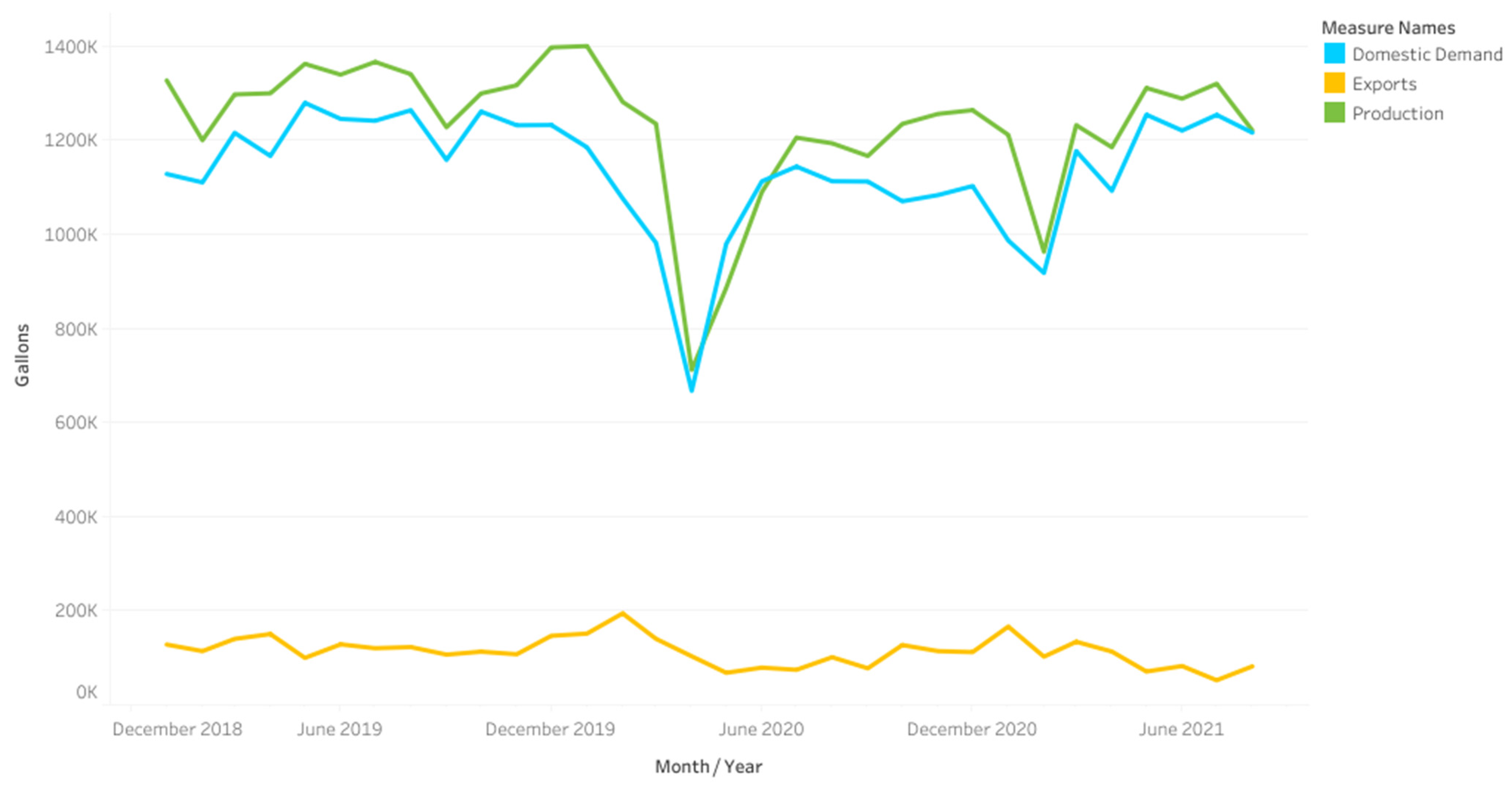
2.4. Demand and Supply in Ethanol Market

Ethanol is ethyl alcohol produced from fermentation and distillation of sugar or starch. In the US, ethanol is made from corn and accounts for approximately 70% of the energy value of gasoline (Hurt et al. 2006). Approximately 205 ethanol plants across the US produce roughly 15.8 billion gallons per year (US Grains Council 2021). This estimated amount exceeds the amount required by US consumers and industry (US Grains Council 2021). Historical data from December 2018 to June 2021 show that the US supply of ethanol exceeded domestic demand for most of this period (Figure 1). This indicates that there is excess production in the US ethanol market. Therefore, sellers may get rid of this surplus by exporting to other countries or reducing the price for local buyers.

3. Structure of Agriculture and Energy Markets

The interconnected characteristics of markets, such as the number of buyers and sellers, the level and forms of competition, the extent of product differentiation, and ease of entry into and exit from the market, define the structure of markets. Markets are grouped into perfectly competitive and imperfect markets based on the level of competition between buyers and sellers. When analyzing any policy, it is important to consider the type of market environment since it affects market outcomes through its impact on motivations, opportunities, and decisions of economic actors participating in the market (Fischer 1997). For instance, in a market with few sellers relative to buyers, sellers can influence prices by selling more or less. At the same time, if there are few buyers relative to sellers, buyers can influence prices by purchasing more or less of the commodity. Therefore, the extent and characteristics of competition in markets affect choice behavior among actors (Fischer 1997). Moreover, trading institutions and methods of delivery may impact market outcomes. Menkhaus et al. (2003) find that market outcomes vary significantly between markets where the trading institution is a double auction, English auction, or private negotiation. Additionally, they find that whether the good is produced prior to trading (called advance production) or produced after a trade (forward delivery) impacts observed market outcomes.

In this study, we analyze subsidy incidence in markets when forward delivery contracts are negotiated privately between parties, and there are relatively few buyers compared to sellers in the market. This form of trading institution and delivery method, as well as the concentration of buyers relative to sellers, is observed in various agricultural and energy market environments (Menkhaus et al. 2003; Menkhaus et al. 2007; Goodhue and Russo 2012; Isola 2012). Therefore, we construct laboratory experiments that parallel relevant features of the actual agricultural and energy market environment and control certain unobserved factors that might impact the ability to empirically analyze subsidy incidence. Unlike previous research conducted on subsidy incidence, we consider a situation where both sides of the market are subsidized, i.e., both buyers and sellers in the market receive subsidies. This allows us to examine the impacts of government policies that subsidize both production and consumption of energy at the same time.3

Based on the theory that subsidy payments will cause a change in market outcomes such as prices and quantities, and behavioral theory of framing associated with tax and subsidy incidence, we developed three hypothesis to drive our analysis:

Hypothesis 1 (H1).

Ho: Subsidizing both sides of the market does not affect market outcomes or incidence.

Hypothesis 2 (H2).

Ho: Framing income transfer payments as subsidy payments does not affect market outcomes or incidence of payments.

Hypothesis 3 (H3).

Ho: Asymmetry of buyers relative to sellers does not impact subsidy incidence or market outcome.

4. Experimental Design

The experiment consisted of a minimum of twenty trading periods, and each trading period contained three one-minute bargaining rounds. Participants were recruited from undergraduate and graduate business and economics programs.4 A recruitment e-mail was sent to students in agricultural and applied economics, economics, or College of Business degree programs informing them of upcoming experimental sessions and how to register for potential participation. An individual was selected to be a participant if he or she has not previously participated in the experiment and had appropriately responded to the recruitment e-mail. Once individuals were registered for participation, they were provided with information about the date and time of the experiment session they were in. Second, an email was sent to the registered individuals as reminder and confirmation of their participation. Finally, on the day of the experiment, all individuals are asked to confirm their details and sign a consent form before starting the experiment. We used different participants for each experimental session to address issues caused by using the same participants across multiple replications (Charness et al. 2012).

Before the experimental session began, instructions concerning market rules, design, profit, earnings calculations, and description of computer screens they would see were presented to participants via a PowerPoint presentation (see Appendix A for example PowerPoint instructions and screenshots used). After instructions were presented, participants were given the opportunity to ask questions. Once participants indicated they were ready to begin the experiment, participants logged into the computerized market which randomly assigned their role as buyer or seller. Participants remained in the same role (buyer or seller) throughout the experimental session. Once participants were assigned their respective roles, a practice session was conducted. The practice session utilized different redemption and unit cost values than the real experiment. We made sure all participants were comfortable with procedures in the practice session and were given the opportunity for additional practice sessions if they were not comfortable. The actual experiment began after each participant indicated they were comfortable with moving into the real experiment and had no further questions. The participants were randomly matched as buyers and sellers during each bargaining round for each trading period. This was done to prevent the formation of reputations among participants (Menkhaus et al. 2007). In addition, participants were requested to refrain from talking and using their phones during the experimental session (Nagler et al. 2013). This enabled us to ensure anonymity and independence in the market.

During the experiment, buyers and sellers enter bids or offers via a computer network for a maximum of one minute per each of three bargaining rounds in a trading period. Buyers can increase their bids without waiting for sellers to respond, while sellers can also decrease their offers without waiting for buyers. The commodity traded in this market is referred to as a “unit”. Matched buyers and sellers negotiate for trade price per unit. Prices and earnings in the market are denoted by an artificial currency called tokens, where 1 token is equivalent to $0.01. Trade occurs in the market when both buyers and sellers agree on a price. Participants were not informed about when the experiment would end in order to avoid any strategic behavior in the final trading period (Nagler et al. 2013). However, they were told a random stop was in place, and the probability of ending the experiment was 1 in 5, while the probability of continuing to the next trading period was 4 in 5 after the 20th trading period. Each participant received a cash payment based on his or her earnings, in addition to a participation fee of $10 once the experimental session ended.

Given our research required multiple treatments and had a limited budget we used a minimum of three replications per treatment. After three replications for each treatment were completed, price and trade quantities were graphed and visually appraised to ensure potential treatment means were not being inappropriately influenced by potential outlier replications. If a replication were deemed as being very different visually compared to the other two replications, an additional two replications were completed to ensure the general tendency related to treatment effects was captured in the replications. All data from all completed replications were used for the analysis. The replications for a base treatment of no subsidy was conducted for a previous research project and had nine replications.

Table 1. Treatments conducted in the experiment.

Treatments	Number of Buyers		Number of Sellers		Number of Replications
1	4	Buyers with no subsidy	4	Sellers with no subsidy	9 Replications
2	4	Buyers with subsidy	4	Sellers with subsidy	5 Replications
3	4	Buyers shift RV	4	Sellers shift cost	3 Replications
4	2	Buyers with no subsidy	4	Sellers with no subsidy	3 Replications
5	2	Buyers with subsidy	4	Sellers with subsidy	3 Replications
6	2	Buyers shift RV	4	Sellers shift cost	5 Replications

shows the various treatments conducted in the experiment.

The base treatment consists of four buyers and four sellers, with no subsidy to buyers and sellers (Table 1). This treatment helps to predict the equilibrium price and quantity in the market when there are no subsidies. This no-subsidy treatment also allows for comparing how the market might be impacted under a subsidy policy (Nagler et al. 2013). The second treatment has four buyers and four sellers, with each buyer and seller receiving a subsidy (Table 1). The purpose of this treatment is to investigate the nature of subsidy incidence when both buyers and sellers receive subsidies, and the number of market participants is symmetric. In the third treatment, we shift both redemption value and cost curves by 20 tokens per unit for four buyers and four sellers, respectively. The redemption value is the maximum amount of money buyers are willing to pay for the unit, while the cost is the marginal cost for producing each unit. Our third treatment helps us to test for framing issues in the market, i.e., do market participants behave differently when the payment is described as a subsidy versus an equivalent shift in redemption and cost schedules.

We concentrate the market by reducing the number of buyers from four to two, with each buyer having a double redemption schedule for the remaining treatments. Doubling the redemption schedule of the two buyers ensured predicted equilibrium from supply and demand schedules were the same for the relevant subsidy treatment which did not have concentrated buyers. As previously mentioned, agricultural and energy markets may have one or few big buyers relative to many sellers. Thus, the double schedules in these treatments help us to represent a concentrated market structure and also maintain the predicted equilibrium in the market. The treatments with asymmetric numbers of buyers are conducted to understand how such market structure issues may impact subsidy incidence. Therefore, our fourth treatment has two buyers and four sellers with no subsidy given to either buyers or sellers. This provides an understanding of how an asymmetric number of buyers relative to sellers impacts markets outcomes in the absence of subsidies. The fifth treatment has the same number of buyers and sellers as our fourth treatment, but both buyers and sellers receive a 20 token per-unit subsidy. The fifth treatment allows us to assess the subsidy impacts when there are asymmetric buyers relative to sellers in the market. For the final treatment, we shift both redemption value and cost schedules by 20 tokens per unit for the two buyers and four sellers in order to investigate potential framing issues in the concentrated market.

5. Data and Econometric Model

We collected data on quantities traded, trade prices, buyer earnings, seller earnings, and total earnings for each experimental session. The quantity traded is the total number of units sold in each trading period, while the trade price is the average price for each trading period. Buyers’ earnings for a traded unit equals the difference between what the buyers pay for the unit and the given redemption value for that unit. The reported data for buyer earnings reflect the average earnings received by buyers for each trading period across the traded units. The amount sellers earn per unit is the difference between the negotiated unit price and the unit cost. Thus, seller earnings are the average earnings received by each seller across the units traded for each trading period. Total earnings are the total profits extracted in the market for each trading period, which is the sum of buyers’ and sellers’ earnings; it provides a measure of total welfare and can be used as a measure of efficiency when compared to the total predicted surplus that is available.

We analyzed the data both graphically and statistically. The statistical analyses were done using a convergence model. To test our hypotheses, we focus on central tendencies across treatments. We construct a balanced panel using data from trading periods 1 through 20. The average of the data across each replication for each treatment is used to minimize individual influences in experimental sessions.5 The convergence model describes the starting points and convergence of the asymptotes of market outcomes for the treatments. The parameter estimates for the asymptotes are used to conduct tests for statistical differences in variables of interest across treatments (Nagler et al. 2013). We used the following convergence model based on Ashenfelter et al. (1992) and modified by Menkhaus et al. (2007):

$$Z_{it}=B_0\left[\frac{\left[t-1\right]}{t}\right]+B_1\left(\frac{1}{t}\right)+{{\displaystyle \sum }}_{j=1}^{i-1}{\alpha }_j{B}_j\left[\frac{\left(t-1\right)}{t}\right]+{{\displaystyle \sum }}_{j=1}^{i-1}{\beta }_j{D}_j\left(\frac{1}{t}\right)+u_{it}$$

(1)

where $Z_{it}$ is the variable of interest such as average price or units traded for each of the t trading periods 1, … 20 in treatment i; $B_0$ is the predicted asymptote of the dependent variables for the base and $B_1$ is the starting level of the dependent variable for the base treatment; ${\alpha }_j$ and $B_j$, respectively, are adjustments to the asymptote and starting level for each of the j treatments in relation to the base; $D_j$ is a dummy variable separating j treatments, and $u_{it}$ is an error term (Bastian et al. 2008).6

We test for differences in the converged price, trade, and earnings across treatments using a t-test in the convergence model. Because the underlying assumption of the t-test is that the data are normally distributed (Neter et al. 1985), we checked for normality by using the Shapiro–Wilk test on the error terms. Following Brown (1997), we also checked for the severity of skewness if the Shapiro–Wilk test indicates normality is potentially violated. Brown (1997) suggests that as long as the data are not severely skewed, the t-test is robust. When normality is violated, and the error terms indicate severe skewness, we average the last five trading periods across the replications and conduct a non-parametric (Wilcoxon) test to compare treatment means. The averages from the last five trading periods across the replications provide a good estimate of the convergence level and has been used in previous literature as a standard (Nagler et al. 2013).

6. Results

6.1. Prices

Figure 2 summarizes the average prices for each treatment. In our base treatment, with four buyers, four sellers, and no subsidy, the average price starts from 70 tokens and fluctuates approximately 75 tokens across the trading periods. This average is below the predicted equilibrium price of 80 tokens. With a per-unit subsidy of 20 tokens paid to both buyers and sellers (4B4S), prices generally fall below the base treatment after the 10th trading period (Figure 2). Prices converge to approximately 71 tokens in this treatment. However, when we frame subsidy payments as a shift in both unit costs and redemption values (revised schedules) by 20 tokens, the average price reached approximately 78 tokens even though the predicted equilibrium is the same for this treatment as the subsidy treatment. This suggests that individuals respond to how the subsidy is framed.

When the market is concentrated to two buyers and four sellers, with no subsidy, average prices are generally below the 4B4S no subsidy treatment but converge to similar levels in the last two trading periods (Figure 2). The average price level in this treatment ranges between 67–74 tokens. This seems consistent with our priori expectation that, as the number of buyers becomes asymmetric relative to sellers, prices will generally be depressed below the 4B4S base treatment. When both buyers and sellers receive subsidies of 20 tokens per unit, prices rise above the no subsidy case and average between 76 and 83 tokens (Figure 2). When both unit cost and redemption value (revised schedules) are shifted by 20 tokens in the market, prices again increase over the subsidy case and converge to 85 tokens in the final trading period.

6.2. Trades

For the base treatment, trades averaged and converged to approximately 14 units (Figure 3). However, with a per-unit subsidy of 20 units to each side of the market, average trades per period are approximately 19 to 20 units. This is expected because subsidies effectively reduce unit costs of sellers, thereby shifting out their individual supply curve. Buyers’ demand curves are also shifted out given the effective increase in their redemption schedules. Interestingly, the highest trade levels occur in the 4B4S treatment, where both buyer and seller schedules are increased by 20 tokens per unit. Trades generally averaged approximately 21 tokens. Again, this tends to suggest that there may be a framing effect associated with the income transfer being presented as subsidies.

In the buyer-concentrated treatments (2B4S), we observe that trade levels are relatively lower than the 4B4S treatments. With no subsidy payment, trades averaged approximately 11 units and finished slightly higher in the last trading period (Figure 3). Compared with the base treatment (4B4S) with no subsidy, trade levels decreased in this treatment. However, with the subsidy payment to buyers and sellers (2B4S), trades averaged between 15 and 16 units and finished at approximately 17 units in the final trading period. The revised schedules treatment (2B4S) generated the highest trades, averaging approximately 18 to 19 units per trading period.

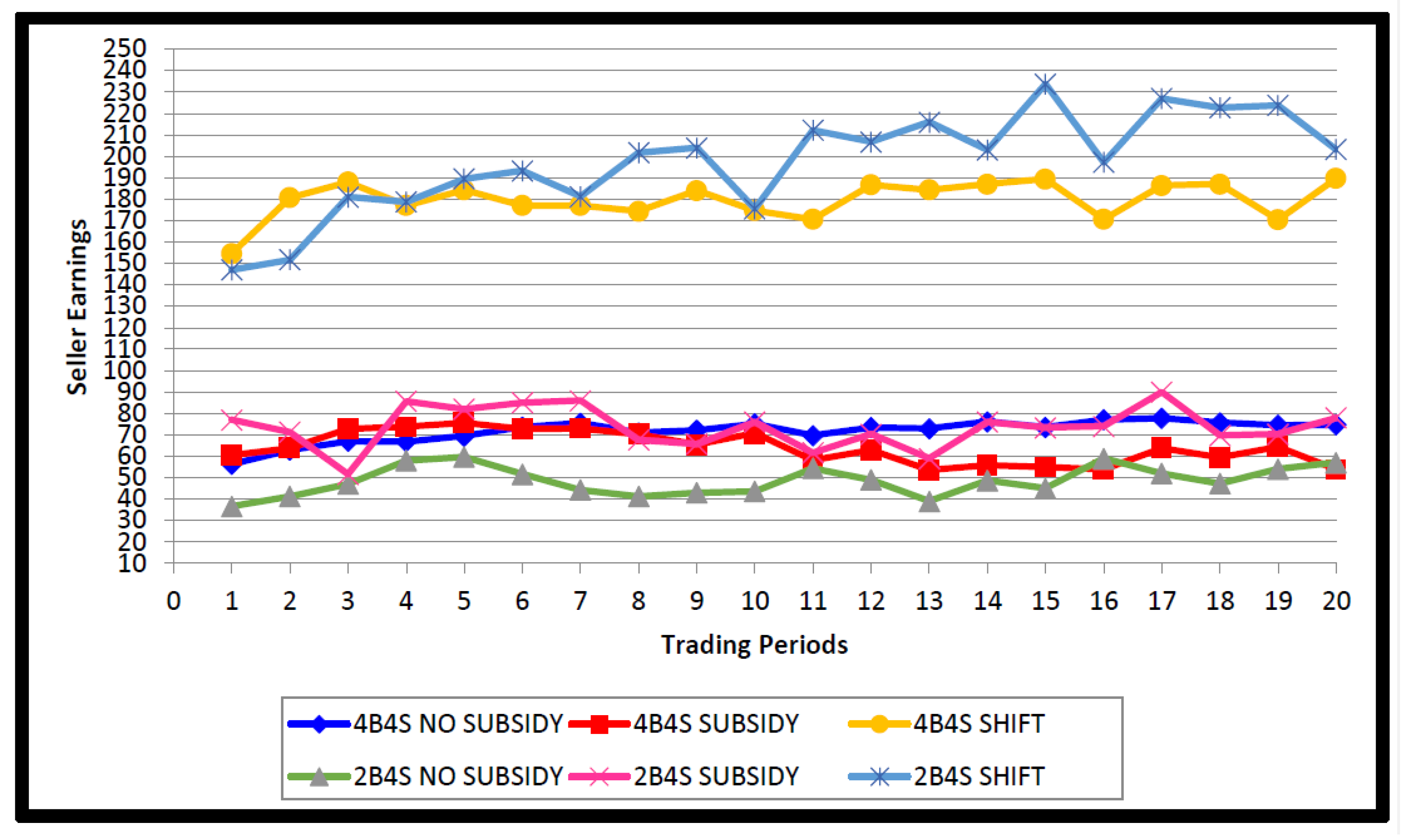
6.3. Seller Earnings

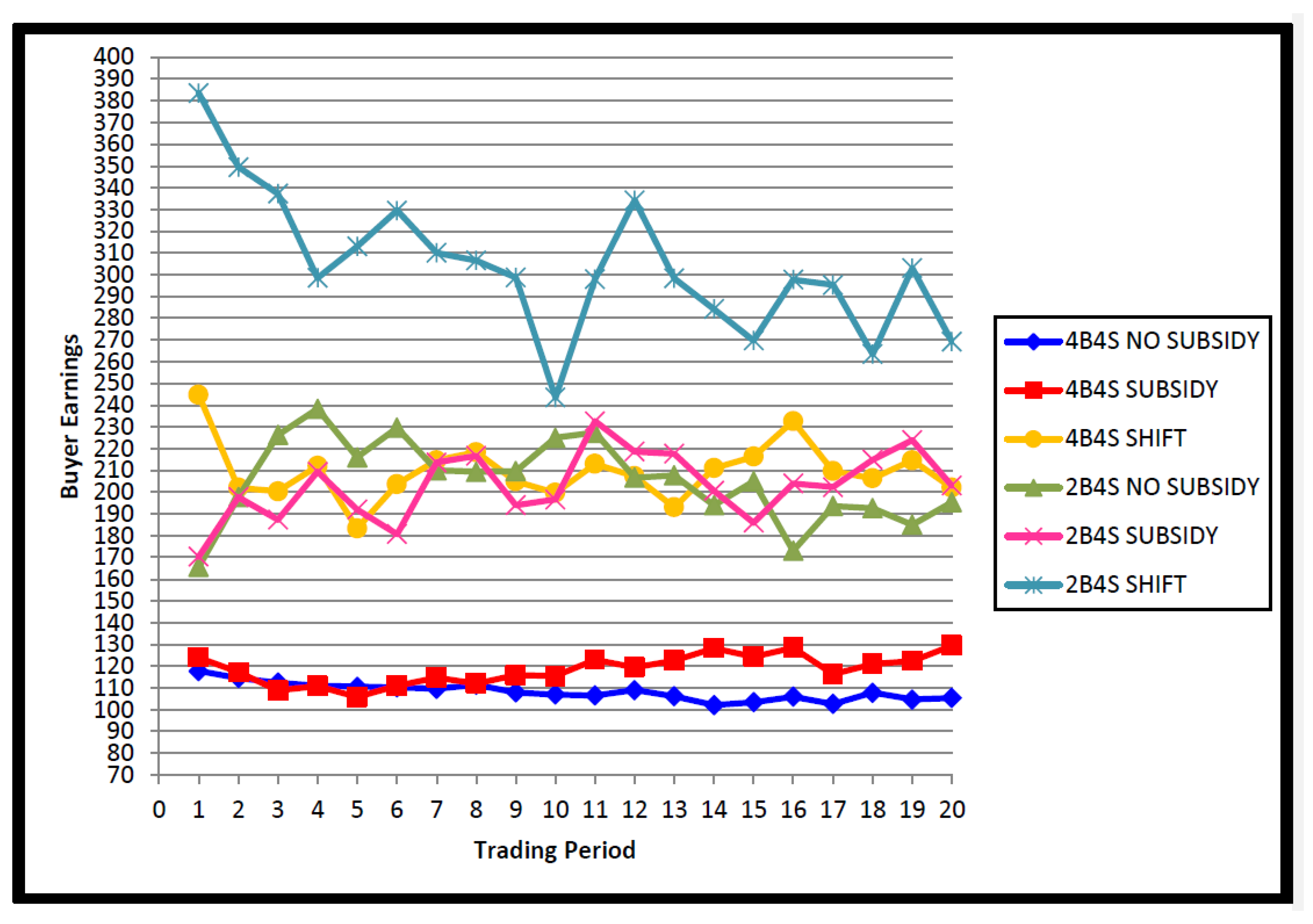
Seller earnings (unsubsidized) equal the sum of the difference in negotiated price and unit cost for the units traded during a trading period (averaged across replications). Seller earnings are generally low in the 2B4S no subsidy treatment, averaging approximately 40 to 50 tokens (Figure 4). However, in the 4B4S no subsidy treatment, seller earnings averaged approximately 75 tokens after the 15th trading period. With a per-unit subsidy of 20 tokens, seller earnings decreased in the 4B4S treatment but increased in the 2B4S treatment (Figure 4). The decrease in earnings reflects the low trade prices in the 4B4S treatment. Seller earnings increased drastically to approximately 180–200 tokens when both cost and redemption schedules were shifted. This is due to the higher prices and quantities traded in the market. Hence, the type of subsidy payment or incentive framing does matter.

6.4. Buyer Earnings

Buyer earnings equal the sum of the difference in redemption value and negotiated price for the units traded during a trading period (averaged across replications). Buyer earnings are low in the 4B4S no subsidy and subsidy stacking treatments (Figure 5). This reflects the lower trade levels we observed. When we compare buyers to sellers, we observe that buyers generally benefit more from the subsidy stacking treatments than sellers. For our revised schedules treatments, buyer earnings are high in the 2B4S case reflecting more surpluses available and more trades even though prices were high in this treatment. Buyer earnings are generally high in the concentrated market treatments as compared to the symmetric market treatments. This is likely due to the fact that buyers are trading two schedules in our concentrated treatments.

When subsidies are stacked in the concentrated market, buyer earnings are generally similar to the no subsidy case. Comparatively, buyer earnings are generally higher than seller earnings across the treatments; buyers tended to be better off in the concentrated market relative to the four buyers and four sellers (4B4S) market treatments. However, on a per-schedule basis (i.e., 2B4S earnings divided by 2), buyer earnings are similar to the 4B4S treatment.

6.5. Total Earnings

Total market earnings is the total amount of surplus or profit made in the market by trading. It measures the level of efficiency in the market. In our base treatment (4B4S), with no subsidy, total market earnings averaged approximately 700 tokens per trading period (Figure 6). This is well below the predicted surplus of 800 tokens in the market. When both buyers and sellers receive the subsidy, total earnings are relatively unchanged, averaging approximately 700 tokens (Figure 6). In the revised schedules treatment, market surplus averages much higher. The predicted surplus for these treatments is 1680 tokens. The 4B4S revised schedule treatment is the most efficient, with the average surplus extracted averaging close to 1600 tokens. In our buyer-concentrated market (2B4S), the revised schedules treatment generated the highest surplus but lower than the 4B4S treatment averaging near the 1400 token level. This represents approximately 83% of the total predicted surplus of 1680 tokens compared to over 90% in the 4B4S treatment. Market surplus extracted from the no subsidy and per-unit subsidy treatments in the buyer-concentrated market averaged approximately 600 and 700 tokens, respectively. Total earnings in the per-unit subsidy treatment (2B4S) are similar to what we observed in the 4B4S no subsidy and subsidy treatments (Figure 6).

7. Estimates from the Convergence Model

7.1. Prices

Prices in the 4B4S no subsidy treatment converged at 74.81 tokens (

Table 2. Estimated convergence levels and treatment parameters for market outcomes.

Treatments	Price	Trades	Total	Buyer	Seller	Relative
	(Tokens)	Levels	Earnings	Earnings	Earnings	Earnings
4 Buyers and
4 Sellers
No Subsidy	74.81	13.93	725.16	104.72	75.69	−29.34i
						(−29.29) a–c,f
Subsidy	73.38 a	19.57 *,a	731.97 a	118.76 *,a	63.53 *,a,c	−55.41i *
	77.28 *,b,c	20.93 *,b	1555.55 *,b	203.33 *,b,c	183.54 *,b	(−64.44) b–e
Shift R.V./Cost						−20.30 i
						(−32.26) c
2 Buyers and
4 Sellers	71.53 *,a	11.71 *,c	632.01 *,c	211.54 *,c,d	51.28 *,a	−159.42 i,*
No subsidy
				[105.77]		(−134.07) d,e
Subsidy	79.48 *,c	15.85 *,d	718.37 a	209.94 *,d,b	73.80 c	−136.76i *
				[104.97]		(−133.27) e,f
Shift R.V./Cost	83.78 *,d	18.45 *,e	1338.44 *,d	303.42 *,e	182.94 *,b	−120.49 i,*
				[151.71]		(−117.20) f,b

* Indicates that the convergence level for the treatment is significantly different from the base treatment, 95% confidence level. ^a–f Same letters indicate no significant difference between the convergence levels, 95% confidence level. [ ] Indicates converged earnings estimate divided by two for a per schedule estimate. ⁱ Violates normality. ( ) Indicates the means of last five trading periods.

). This is 5.19 tokens below the predicted market equilibrium of 80 tokens. This could be due to matching risk and bargaining advantage for buyers relative to sellers in the private negotiation market (Menkhaus et al. 2003). With a per-unit subsidy of 20 tokens to both sides of the market, prices converged at 73.38 tokens, not significantly different from the no subsidy treatment. When both buyer and seller schedules are revised, negotiated prices converged at 77.28 tokens (Table 2). Compared to the per-unit subsidy treatment, we observed that prices, in addition to trades and earnings, are high when we frame the payment as a shift in schedules. Therefore, our results confirm that the way payments are framed can affect market outcomes. We, therefore, reject our null hypothesis (Ho 2), which suggests that framing the subsidy payment as a government payment versus a shift in the unit redemption and cost schedules does affect market outcomes. Hence, framing matters in subsidy incidence.

For the concentrated markets, prices in the 2B4S treatment converged at 71.53 tokens when no subsidy was paid to buyers and sellers. This is the lowest price observed in all the treatments. However, this is expected because buyers tend to have a bargaining advantage over sellers in a buyer-concentrated market. Statistically, the prices in our 2B4S treatment with no subsidy are not different from what we observed in the 4B4S no subsidy and per-unit subsidy treatments (Table 2). Interestingly, with a per-unit subsidy and bargaining advantage for buyers, buyers negotiated for high prices in the subsidy treatment. The convergence model estimated the price to be 79.48 tokens (Table 2). When we compare this outcome to buyer and seller earnings, we observe that buyers benefited more than sellers irrespective of the high prices negotiated. However, buyer earnings are not significantly different from the no subsidy treatment. With revised schedules for buyers and sellers, the estimated market price for the 2B4S is 83.78 tokens. As observed in Figure 2, this is the highest negotiated price in all six treatments. The results from the experiment indicate that subsidizing both sides of the market at the same time tend to affect market outcomes, i.e., earnings, trades, and prices (Table 2). Therefore, we reject our null hypothesis (Ho 1), which states that subsidizing both sides of the market does not affect market outcomes. It is interesting to note that adding subsidies or income transfers via shifting schedules seems to counteract the effect of concentrating the market.

7.2. Trades

Trades in all the treatments are statistically different from each other. In the base treatment, trades converged at 13.93 units and increased to 19.57 units when buyers and sellers received the subsidy (4B4S) (Table 2). When we revised both buyers’ and sellers schedules, trade levels converged at 20.93 units per period, significantly higher than the base (Table 2). As expected, lower levels of trades are observed in the buyer-concentrated market than the 4B4S treatment with no subsidy (Table 2), as buyers should have a bargaining advantage. This is in conjunction with lower observed prices. With no subsidy payment, trade levels per period converged at 11.71 units. This is lower than the predicted equilibrium quantity of 16–20 units, and significantly lower than the 4B4S base. We believe this contributed to the low seller earnings observed in this treatment (Table 2). The per-unit subsidy payment impacted the concentrated market by increasing trade levels to 15.85 units. Trades observed in the revised schedule treatment are estimated to be 18.45 units. Overall, comparing across treatments in the concentrated market relative to the symmetric market, quantities traded are lower, reflecting buyer asymmetry and increased matching risk. The lower trades observed in the buyer-concentrated market contribute to the higher earnings for buyers since they purchased less units while trading on double unit schedules and keeping some of the subsidies. However, on a per-schedule basis, buyer earnings are similar to what we observed in the subsidy and no subsidy treatments in the 4B4S market structure.

7.3. Total Earnings

Total market surplus extracted from the revised schedule treatment (4B4S) converged at 1555.55 tokens (Table 2). This is consistent with our observation in Figure 4, where the last five trading periods averaged approximately 1550 tokens. This estimate represents the highest surplus extracted in all the six treatments (Figure 5). The per-unit subsidy treatment in the 4B4S market structure generated a surplus of 731.97 tokens, while the no subsidy treatment converged at 725.16 tokens (Table 2). Though market surplus in the no subsidy treatment is more than the subsidy treatment, the estimates are not statistically different. This is also consistent with what we observed in Figure 5. In our 2B4S market structure, the market surplus converged at 1338.44 tokens for the revised schedule treatment. This is 341.56 tokens lower than the predicated market surplus of 1680 tokens in the market. The total market surplus observed in the no subsidy treatment converged at 632.01 tokens, which is the lowest among all the treatments (Table 2 and Figure 6). The per-unit subsidy treatment converged at 718.37 tokens, not significantly different from the base treatment (4B4S no subsidy) and the per-unit subsidy treatment (Table 2).

7.4. Seller Earnings

The convergence estimates for seller earnings (unsubsidized) are 75.69 tokens and 63.53 tokens for the 4B4S no subsidy and per-unit subsidy treatment, respectively (Table 2). This is consistent with what we observed in the graph (Figure 4) and indicates that sellers were worse off with the subsidy payment as sellers essentially bargain for lower prices and allow buyers to bargain away some of the subsidy; their unsubsidized earnings decreased by 16.1 percent as a result of the subsidy. Thus, buyers were able to extract approximately 61 percent of the subsidy given to sellers. The estimate for the revised schedules treatment is 183.54 tokens. In the 2B4S market structure, seller earnings are very low when no subsidy is paid to buyers and sellers. The convergence model estimates seller earnings with no subsidy at 51.28 tokens compared to 75.69 tokens in the 4B4S case. However, when the subsidy is paid to buyers and sellers, seller earnings (unsubsidized) increased to 73.80 tokens, i.e., a 43.9 percent increase in earnings. Seller earnings estimated by the convergence model for the revised schedules treatment for 2B4S is 183.94 tokens (Table 2). This is almost the same as the estimate in the 4B4S revised schedule treatment. Statistically, there is no difference between these estimates (Table 2). Additionally, seller earnings are not statistically different between the 4B4S and 2B4S subsidy treatments. However, with no subsidy payment, seller earnings are significantly different in both markets (Table 2).

7.5. Buyer Earnings

Buyer earnings in the 4B4S no subsidy treatment converged at 104.72 tokens per period. This increased to 118.72 (not including the subsidy payment) tokens in the subsidy treatment. Compared to sellers’ earnings, buyers’ earnings increased by approximately 13.4 percent, while seller earnings decreased by 16.1 percent when we subsidized both sides of the market. Buyer earnings in the revised schedules treatment converged at 203.33 tokens per trading period, representing an increase of approximately 94 percent in buyer earnings. When we concentrated the market to 2B4S, buyer earnings converged at 211.54 tokens and 209.94 tokens for the no subsidy and per-unit subsidy treatments, respectively (Table 2). These estimates are not statistically different from each other. When we shifted the costs and redemption values by 20 tokens, buyers earned more than sellers. Buyer earnings converged at 303.42 tokens (Table 2), statistically different from all the other treatments. This indicates that framing affects the distribution of subsidy benefits. On a per-schedule basis, we observed that buyer earnings in our 2B4S no subsidy treatment converged at 105.77 tokens, similar to the base (4B4S no subsidy). However, with a per-unit subsidy of 20 tokens, buyer earnings (per-schedule basis) decreased slightly in our 2B4S market compared to the 4B4S subsidy treatment (Table 2). When we revised the schedules in our 2B4S market, buyer earnings on a per-schedule basis converged at 151.71 tokens, less than what we observed in the 4B4S case (Table 2).

7.6. Relative Earnings

Relative earnings are calculated as seller minus buyer earnings. This measures the earning advantage in the market; negative earnings indicate buyer advantage, and positive indicate seller advantage in the market (Nagler et al. 2013). The results generally show that buyers are better off across all treatments than sellers as the relative earnings are all negative (Table 2). In the base treatment (4B4S), with no subsidy payment, relative market earnings indicate average buyer advantage of 29.34 tokens over seller (Table 2). With a per-unit subsidy of 20 tokens, buyer advantage increases further to 55.41 tokens (without the subsidy payment), indicating an increase of approximately 89 percent. This occurs as sellers receiving the subsidy negotiate away much of the potential income from the subsidy. However, this advantage falls when schedules are revised by 20 tokens for both buyers and sellers. Buyer advantage falls to 20.30 tokens (without subsidy payment).

As expected, buyer advantage is higher in the 2B4S treatments than the 4B4S treatments. The no subsidy treatment indicates a 159.42 tokens advantage for buyers. Interestingly, this advantage falls when buyers and sellers receive the per-unit subsidy. The estimated relative earnings are 136.76 tokens (Table 2), which is approximately 23 tokens less than what we observed in the no subsidy treatment. Relative earnings in the revised schedules treatment also show a decrease in buyer advantage of approximately 40 tokens compared to the no subsidy treatment. However, as mentioned earlier, buyer advantage is higher in the 2B4S market than in the 4B4S market structure. Our results, therefore, show that asymmetry buyers relative to sellers does influence market outcomes. Hence, we reject our null hypothesis (Ho 3) that asymmetry of buyers relative to sellers does not impact subsidy incidence or market outcome.

8. Discussion

In general, the results above show that buyers tend to do better in all treatments than sellers (Table 2). This is likely a function of the private negotiation trading institution and consistent with past research findings (Menkhaus et al. 2003). When we concentrate the market to two buyers and four sellers, buyers generally increase their earnings compared to the same treatments with an equal number of buyers and sellers. This could be due to the fact that in addition to the subsidy payment, buyers have a bargaining advantage relative to sellers as a result of their size in the market as well as increased matching risk for sellers, i.e., the ability of sellers to match with a buyer to trade is cut in half for each bargaining round in a trading period. On the other hand, when we consider buyer earnings on a per-schedule basis, buyers tend to do better in the equal number of buyers and sellers market than the concentrated market.

In addition, in spite of the high prices negotiated in the concentrated market, the number of trades is reduced so as to enable buyers to increase their earnings. We believe that buyers increase their earnings in the concentrated market by reducing their purchases to compensate for the higher negotiated prices in the market. This may be partially due to the double schedules that buyers face in our experimental design. Buyers have two units they can trade at each redemption value, so margins are highest on the earlier units in their schedule. Thus, buyers can attract units with higher prices and make a relatively good surplus on units earlier in their double schedules.

The high prices in our schedule shift treatments suggest that there is a framing effect in both market structures compared to the subsidy treatments. This result confirms the suggestion of a potential framing effect posited by Nagler et al. (2013). However, our result is in contrast to Rahman et al. (2019), who found no framing effect regarding subsidy incidence in a privately negotiated laboratory market. While market structures and base supply and demand schedules are the same across those two papers, a difference in delivery methods does exist. Rahman et al. (2019) test subsidy incidence in a privately negotiated market with advance production or spot delivery. Overall, this evidence would suggest that in market environments dominated by private negotiation, delivery method may well impact the potential for a framing effect associated with policies using subsidies.

In terms of market surplus, the results show that relatively more surplus is extracted when the market is highly competitive than when concentrated (Table 2). Additionally, these results indicate that if the policy goal is to increase the level of production and consumption of a commodity, then support programs present in the type of market environment modeled here will be more efficient when designed in a way that will shift the cost and demand curves for buyers and sellers rather than framed as a direct subsidy payment.7 Furthermore, this is true whether the market structure is concentrated or not. In summary, our results show that when subsidizing both sides of the market, framing effects may matter. When markets are buyer concentrated, subsidy distributions generally tend to favor buyers. This general conclusion is relatively consistent with simulation results by Saitone et al. (2008) examining ethanol subsidization. They conclude distribution of the subsidy tended to favor upstream and downstream oligopsonists compared to corn producers in the corn supply chain. However, their results did not include simultaneous subsidies received by corn producers. It is interesting that when subsidizing both sides of the market, i.e., subsidy stacking, our results suggest that the impacts of concentration are potentially reduced.

9. Conclusions

Government policies employ different programs such as subsidies to increase efficiency in markets and enhance societal welfare. Oftentimes, multiple agents in different market roles may receive some type of income transfer in agricultural and energy-related markets. For example, ethanol producers have benefitted from subsidies and blend mandates, while corn producers may receive subsidies through various policy mechanisms. People who are involved in market transactions with the beneficiary may receive part of the subsidy. This phenomenon is referred to as subsidy incidence. In this study, we investigate subsidy incidence when both buyers and sellers receive a subsidy in a market environment dominated by private negotiation and forward delivery with a structure where there are few buyers relative to sellers.

We design a laboratory market to mimic the structure found in various agricultural and energy markets, such as biofuel markets, and collect data on market transactions for the analysis. Two separate markets structures are designed for the experiment. The first market structure has an equal number of buyers and sellers, while the second market has few buyers relative to sellers. We conducted six treatments for approximately twenty trading periods, and each trading period consisted of three bargaining periods. The first treatment is the base treatment, which consists of four buyers and four sellers in which none of the participants receive a subsidy. The second treatment has four buyers and four sellers, with each buyer and seller receiving a per-unit subsidy of 20 tokens. In the third treatment, we shift both redemption value and cost curves by 20 tokens for the four buyers and four sellers, respectively, to see if there is a difference in outcomes when participants receive the income transfer as subsidies versus as a shift in the supply and demand curves in the market. We repeat these conditions for treatments four, five, and six, except the number of buyers is reduced from four to two, each having double redemption schedules.

The results from the experiment indicate that buyers generally benefit more than sellers when both receive a subsidy in the market environment modeled. With a per-unit subsidy of 20 tokens paid to each side of the market, buyer earnings increased by 13.4 percent in the four buyers and four sellers treatment as more units were traded and prices converged to levels similar to the no subsidy treatment. On the other hand, seller earnings decreased by 16.1 percent due to the relatively low prices negotiated. In the buyer-concentrated market, buyers and sellers negotiated for higher prices when they both received a per-unit subsidy of 20 tokens. However, units traded in this market are relatively low compared to the same treatment with four buyers and four sellers. On a per-schedule basis, our results show that buyers benefitted more from the subsidy payment in the 4B4S market than in the 2B4S market structure. When we revised buyer and seller schedules by 20 tokens per unit, prices and quantities traded increased as well as earnings for both buyers and sellers in each market. In the 4B4S market structure, prices increased by 3.2 percent and trades 50.6 percent. For our 2B4S market structure, prices increased by 17 percent and 57.6 percent for units traded. Compared with all other treatments, prices, trades, and earnings are highest in the revised schedules treatments.

Our results imply that the way support programs are designed can have an impact on how markets will operate, and both structure and delivery method found in the market environment may affect subsidy influences. Moreover, how the support program is structured may result in different outcomes. Based on our findings, we recommend that, when market environments are dominated by private negotiation and forward contracting, support programs that are meant to encourage production and consumption at the same time should be designed to shift the supply and demand curves of buyers and sellers, respectively, rather than giving a direct subsidy to firms. By shifting the supply and demand curves, our results show that the support program will increase quantities and move prices toward a competitive level, thereby reducing the distortions often created by direct subsidy payments.

References

1. Alm, James. 2010. Testing Behavioral Public Economics Theories in the Laboratory. National Tax Journal 63: 635–58. [Google Scholar] [CrossRef] [Green Version]
2. Andreoni, J., and John Miller. 2002. Giving According to GARP: An Experimental Test of the Consistency of Preferences for Altruism. Econometrica 70: 737–53. [Google Scholar] [CrossRef] [Green Version]
3. Ashenfelter, Orley C., Janet Currie, Henry S. Farber, and Matthew Spiegel. 1992. An Experimental Comparison of Dispute Rates in Alternative Arbitration Systems. Econometrica 60: 1407–33. [Google Scholar] [CrossRef]
4. Bastian, Christopher T. 2019. Evolution toward Private Negotiation as a Dominant Institution in Agribusiness Supply Chains: Implications, Challenges, and Opportunities. Journal of Agricultural and Resource Economics 44: 457–73. [Google Scholar]
5. Bastian, Christopher T., Dale J. Menkhaus, Amy M. Nagler, and Nicole S. Ballenger. 2008. Ex Ante Evaluation of Alternative Agricultural Policies in Laboratory Posted Bid Markets. American Journal of Agricultural Economics 90: 1208–15. [Google Scholar] [CrossRef]
6. Brown, James Dean. 1997. Questions and Answers about Language Testing Statistics: Skewness and Kurtosis. Shiken: JALT Testing & Evaluation SIG Newsletter 1: 20–23. [Google Scholar]
7. Charness, Gary, Uri Gneezy, and Michael A. Kuhn. 2012. Experimental Methods: Between-subject and Within-subject Design. Journal of Economic Behavior & Organization 81: 1–8. [Google Scholar]
8. Cook, Benjamin R. 2010. Essays on Carbon Policy and Enhanced Oil Recovery. Ph.D. dissertation, Economics Department, University of Wyoming, Laramie, WY, USA. [Google Scholar]
9. De Gorter, Harry, and David R. Just. 2010. The Social Costs and Benefits of Biofuels: The Intersection of Environmental, Energy and Agricultural Policy. Applied Economic Perspectives and Policy 31: 4–32. [Google Scholar] [CrossRef] [Green Version]
10. Demmel, Laura. 2008. State Policies in the North Central Region Promotion Ethanol. Available online: https://digitalcommons.unl.edu/cgi/viewcontent.cgi?article=1001&context=ageconundergrad (accessed on 1 October 2021).
11. Fischer, Charles C. 1997. What Can Economics Learn from Marketing’s Market Structure Analysis? Business Quest. Journal of Applied Topics in Business and Economics. Available online: http://www.westga.edu/~bquest/1997 (accessed on 1 October 2021).
12. Fréchette, Guillaume R. 2015. Chapter 7: Experimental Economics across Subject Populations. In The Handbook of Experimental Economics, 2nd ed. Edited by Alvin E. Roth and John H. Kagel. Princeton: Princeton University Press. [Google Scholar]
13. Friedman, Sunder, Daniel Friedman, and Shyam Sunder. 1994. Experimental Methods: A Primer for Economists. New York: Cambridge University Press. [Google Scholar]
14. Gamage, David, Andrew T. Hayashi, and Brent K. Nakamura. 2010. Experimental Evidence of Tax Framing Effects on the Work/Leisure Decision. SSRN Working Paper. Rochester: Social Science Research Network. [Google Scholar]
15. Goodhue, Rachael E., and Carlo Russo. 2012. Modeling Processor Market Power and the Incidence of Agricultural Policy: A Nonparametric Approach. In The Intended and Unintended Effects of US Agricultural and Biotechnology Policies. Edited by Joshua S. Graff Zivin and Jeffrey M. Perloff. Chicago: University of Chicago Press. [Google Scholar]
16. Goodwin, Barry K., Ashok K. Mishra, and François N. Ortalo-Magné. 2003a. Explaining Regional Difference in the Capitalization of Policy Benefits into Agricultural Land Values. In Government Policy and Farmland Markets—The Maintenance of Farmer Wealth. Edited by Charles Moss and Andrew Schmitz. Ames: Iowa State Press, pp. 3–14. [Google Scholar]
17. Goodwin, Barry K., Ashok K. Mishra, and François N. Ortalo-Magné. 2003b. What’s Wrong with Our Models of Agricultural Land Values? American Journal of Agricultural Economics 85: 744–52. [Google Scholar] [CrossRef]
18. Goodwin, Barry K., Ashok K. Mishra, and François Ortalo-Magné. 2012. The Buck Stops Where? The Distribution of Agricultural Subsidies. In The Intended and Unintended Effects of S.US Agricultural and Biotechnology Policies. Edited by Joshua S. Graff Zivin and Jeffrey M. Perloff. Chicago: University of Chicago Press, pp. 15–50. [Google Scholar]
19. Hurt, C., W. Tyner, and O. Doering. 2006. Economics of Ethanol. Extension Publication No. 339. West Lafayette: Purdue University. [Google Scholar]
20. Isola, Wakeel A. 2012. An Analysis of Electricity Market Structure and Its Implications for Energy Sector Reforms and Management in Nigeria. Global Advanced Research Journal of Management and Business Studies 5: 141–49. [Google Scholar]
21. Kirwan, Barrett E. 2009. The Incidence of US Agricultural Subsidies on Farmland Rental Rates. Journal of Political Economy 117: 138–64. [Google Scholar] [CrossRef] [Green Version]
22. Komives, Kristin, Jon Halpern, Vivien Foster, Quentin Wodon, and Roohi Abdullah. 2007. Utility Subsidies as Social Transfers: An Empirical Evaluation of Targeting Performance. Development Policy Review 25: 659–79. [Google Scholar] [CrossRef]
23. Kumar, Radika, Ronald Ravinesh Kumar, Peter Josef Stauvermann, and Pallavi Arora. 2020. Effect of Fisheries Subsidies Negotiations on Fish Production and Interest Rate. Journal of Risk and Financial Management 13: 297. [Google Scholar] [CrossRef]
24. Menkhaus, Dale J., Owen R. Phillips, and Chris T. Bastian. 2003. Impacts of Alternative Trading Institutions and Methods of Delivery on Laboratory Market Outcomes. American Journal of Agricultural Economics 85: 1323–29. [Google Scholar] [CrossRef]
25. Menkhaus, Dale J., Owen R. Phillips, Christopher T. Bastian, and Lance B. Gittings. 2007. The Matching Problem (and Inventories) in Private Negotiation. American Journal of Agricultural Economics 89: 1073–84. [Google Scholar] [CrossRef]
26. Nagler, Amy M., Dale J. Menkhaus, Christopher T. Bastian, Mariah D. Ehmke, and Kalyn T. Coatney. 2013. Subsidy Incidence in Factor Markets: An Experiment al Approach. Journal of Agricultural and Applied Economics 45: 17–33. [Google Scholar] [CrossRef] [Green Version]
27. Nechyba, Thomas. 2011. Microeconomics: An Intuitive Approach with Calculus, 1st ed. Mason: Cengage Learning. [Google Scholar]
28. Neter, John, William Wasserman, and Michael H. Kutner. 1985. Applied Linear Statistical Models: Regression, Analysis of Variance, and Experimental Design, 2nd ed. Homewood: Richard D. Irwin, Inc. [Google Scholar]
29. Parks, Richard W. 1967. Efficient Estimation of a System of Regression Equations when Disturbances are Both Serially and Contemporaneously Correlated. Journal of the American Statistical Association 62: 500–9. [Google Scholar] [CrossRef]
30. Patton, Myles, Philip Kostov, Seamus McErlean, and Joan Moss. 2008. Assessing the Influence of Direct Payments on the Rental Value of Agricultural Land. Food Policy 33: 397–405. [Google Scholar] [CrossRef]
31. Qiu, Feng, Jean-Philippe Gervais, and Barry K. Goodwin. 2010. An Empirical Investigation of the Agricultural Subsidy Incidence on Farmland Rental Rates. Paper Presented at Selected Paper Prepared for Presentation at the Agricultural & Applied Economics Association 2010 AAEA, CAES, & WAEA Joint Annual Meeting, Denver, CO, USA, July 25–27. [Google Scholar]
32. Rahman, Mohammad Maksudur, Christopher T. Bastian, Chian Jones Ritten, and Owen R. Phillips. 2019. Subsidy Incidence in Privately Negotiated Spot Markets: Experimental Evidence. Journal of Agricultural and Applied Economics 51: 219–34. [Google Scholar] [CrossRef] [Green Version]
33. Rasul, Imran, Andrew Leicester, and Peter Levell. 2012. Tax and Benefit Policy: Insights from Behavioral Economics. London: The Institute for Fiscal Studies. [Google Scholar]
34. Ruffle, Bradley J. 2005. Tax and Subsidy Incidence Equivalence Theories: Experimental Evidence from Competitive Markets. Journal of Public Economics 89: 1519–42. [Google Scholar] [CrossRef]
35. Saitone, Tina L., Richard J. Sexton, and Steven E. Sexton. 2008. Market Power in the Corn Sector: How Does It Affect the Impacts of the Ethanol Subsidy? Journal of Agricultural and Resource Economics 33: 169–94. [Google Scholar]
36. SAS. 2008. SAS/ETS 9.2 User’s Guide. Cary: SAS Institute Inc, Available online: http://support.sas.com/documentation/cdl/en/etsug/60372/PDF/default/etsug.pdf (accessed on 2 July 2013).
37. Schechinger, Anne. 2021. Under Trump, Farm Subsidies Soared and the Rich Got Richer Biden and Congress Must Reform a Wasteful and Unfair System. Available online: https://www.ewg.org/interactive-maps/2021-farm-subsidies-ballooned-under-trump (accessed on 1 October 2021).
38. US Grains Council. 2021. Ethanol Production and Exports. Available online: https://grains.org/buying-selling/ethanol-2/ethanol/ (accessed on 1 October 2021).
39. Zelinsky, Edward A. 2005. Do Tax Expenditures Create Framing Effects? Volunteer Firefighters, Property Tax Exemptions, and the Paradox of Tax Expenditure Analysis. Virginia Tax Review 24: 797–834. [Google Scholar]
Figure 1. US supply and demand of ethanol (Source: Renewable Fuels Associations Monthly Ethanol Supply & Demand).
Jrfm 14 00608 g001
Figure 2. Average prices per trading period by treatment.
Jrfm 14 00608 g002
Figure 3. Average quantities traded per trading period by treatment.
Jrfm 14 00608 g003
Figure 4. Average seller earnings per trading period by treatment.
Jrfm 14 00608 g004
Figure 5. Average buyer earnings per trading period by treatment.
Jrfm 14 00608 g005
Figure 6. Average total earnings per trading period by treatment.
Jrfm 14 00608 g006