
A Bayesian Semiparametric Realized Stochastic Volatility Model


Sobey School of Business, Saint Mary’s University, Halifax, NS B3H 3C3, Canada
J. Risk Financial Manag. 2021, 14(12), 617; https://0-doi-org.brum.beds.ac.uk/10.3390/jrfm14120617
Submission received: 2 November 2021
/
Revised: 13 December 2021
/
Accepted: 15 December 2021
/
Published: 19 December 2021
(This article belongs to the Special Issue Financial Markets, Financial Volatility and Beyond)
Abstract
:This paper proposes a semiparametric realized stochastic volatility model by integrating the parametric stochastic volatility model utilizing realized volatility information and the Bayesian nonparametric framework. The flexible framework offered by Bayesian nonparametric mixtures not only improves the fitting of asymmetric and leptokurtic densities of asset returns and logarithmic realized volatility but also enables flexible adjustments for estimation bias in realized volatility. Applications to equity data show that the proposed model offers superior density forecasts for returns and improved estimates of parameters and latent volatility compared with existing alternatives.
1. Introduction
Asset volatility plays a crucial role in many financial problems such as derivative pricing, risk management, and portfolio allocation. The generalized autoregressive conditional heteroscedasticity (GARCH) model introduced by Bollerslev (1986) and stochastic volatility (SV) model formalized by Taylor (1986) are standard econometric tools for estimating and forecasting financial asset volatility. Recent developments in financial econometrics benefit volatility modeling in several aspects. For one thing, the availability of high-frequency data provides realized measures of ex-post volatility, which are data on historical volatility. For another, econometric techniques such as the Bayesian nonparametric mixture enable modeling data in more flexible ways. This paper proposes an extended SV model that utilizes information from both returns and realized volatility (RV) under a flexible Bayesian nonparametric framework. Compared with existing models, the proposed models significantly improve density forecasts of returns and volatility measures.
To better accommodate asymmetric and heavy-tailed features of asset returns, many works have extended the SV model by relaxing the Gaussian distributional assumption. Non-Gaussian innovation distributions used in the SV framework include the Student’s t (Chib et al. 2002; Sandmann and Koopman 1998), normal inverse Gaussian (Barndorff-Nielsen 1997), finite Gaussian mixture (Kim et al. 1998; Mahieu and Schotman 1998) and generalized hyperbolic skew Student’s t (Nakajima and Omori 2012). Recent advances in Bayesian nonparametrics enable modeling data without distributional assumptions. Jensen and Maheu (2010) extends the SV model to its semiparametric version with a nonparametric mixture innovation distribution. Other versions of semiparametric SV models include those in Yu (2012); Delatola and Griffin (2013); Jensen and Maheu (2014) and Virbickaitė and Lopes (2019).
For two decades, estimation of ex-post volatility using high-frequency data has been a very active research topic in financial econometrics. Andersen et al. (2001) and Barndorff-Nielsen and Shephard (2002) show that the RV estimator defined as the summation of squared intraday returns is consistent for ex-post daily volatility in an ideal scenario. In practice, price observations are contaminated with market microstructure noise, which leads to biased RV measures. Zhang et al. (2005) suggest that the average of subsampled RV measures outperforms RV and introduce a two-scales volatility estimator. Barndorff-Nielsen et al. (2008) propose a kernel-based approach for volatility estimation. Other estimators include the realized power variation (Barndorff-Nielsen and Shephard 2004), range-based volatility estimator (Christensen and Podolskij 2007), pre-averaged RV (Jacod et al. 2009) and quasi-maximum likelihood estimator (Xiu 2010). High-frequency volatility estimators quantify latent volatility nonparametrically and provide data on volatility. Maheu and McCurdy (2011) show that jointly modelling returns and RV leads to significant improvements in return density forecasts. Takahashi et al. (2009) propose a realized SV (RSV) model that simultaneously analyzes returns and RV measures. Shirota et al. (2014) and Asai et al. (2017) extend the RSV model to allow for leverage, long memory or asymmetry. Other joint return-RV models include the realized GARCH (Hansen et al. 2012), high-frequency-based volatility (HEAVY) model (Shephard and Sheppard 2010) and Markov switching model with RV (Liu and Maheu 2018).
Compared with return data, ex-post volatility estimates offer more accurate volatility measures but are subjective to estimation bias caused by the market microstructure noise. Takahashi et al. (2009) equip the RSV model with a constant correction term to adjust the estimation bias. Nevertheless, later works such as Bandi et al. (2013) note that the bias in RV could be time-varying due to the variation in market microstructure noise. In addition, most works, including Takahashi et al. (2009), assume that logarithmic RV (logRV) follows a Gaussian distribution. However, Corsi et al. (2008) shows that the volatility of RV is time-varying, and residuals in several logRV models are not normally distributed. Huang et al. (2019) study the option implied volatility and find the volatility of volatility varies over time.
This paper extends the RSV model to its semiparametric version by relaxing assumptions about innovation distributions and RV estimation bias. Such an extension provides two benefits. First, the non-Gaussian features of both return and logRV are better accommodated under the Bayesian nonparametric framework with no distributional assumptions. Following Jensen and Maheu (2010), I incorporate the RSV model with the Dirichlet process mixture (DPM), which is a Bayesian nonparametric mixture model allowing a nonfixed number of clusters. Second, I assume that the RV estimation bias is time-varying. Instead of adjusting the RV bias via a constant parameter, the proposed model adopts a varying correction term to filter out the bias, which facilitates the extraction of volatility information from RV data. I consider three versions of semiparametric RSV models, in which return and logRV processes are influenced by a common DPM, are governed by two independent DPMs, or only the return innovation terms follow a DPM.
The proposed model is evaluated against existing SV models including RSV, SV-DPM, and standard SV and GARCH models with normal or Student’s t innovations. Empirical applications to three U.S. equities (Disney (DIS), IBM, SPDR S&P 500 ETF (SPY)) and one South Korea stock (SK Hynix (SKHY)) disclose the benefit of the proposed extension of the RSV model. The semiparametric RSV model captures stronger volatility persistence and results in a less noisy log volatility process compared with the RSV model. The nonparametric mixture well characterizes skewed and heavy-tailed densities for both returns and logRV, as shown in predictive density plots. In contrast to the semiparametric SV model without RV, the semiparametric RSV model fits the return density using a mixture with fewer clusters. In out-of-sample forecasting, the proposed model significantly improves return density forecasts compared with benchmark models. Incorporating the RSV model with Bayesian nonparametric mixtures also benefits the forecast of logRV densities. Both in-sample and out-of-sample results are robust to the choice of assets, subsample periods, and RV measures.
The remainder of the paper is organized as follows. Section 2 provides a brief summary of ex-post volatility estimation and discusses the data. Section 3 illustrates the proposed models, benchmarks, Bayesian inference, and model comparison. Full sample estimates and out-of-sample forecasting results are reported in Section 4. Section 5 concludes the paper, followed by an Appendix A.
2. Ex-Post Volatility Estimation and Data
2.1. Ex-Post Volatility Estimation
Consider the following stochastic process for logarithmic price :
where is a drift term, stands for the instantaneous volatility, and is a Brownian motion. The integrated variance is the true variance measure of the return over the period and is defined as
Andersen et al. (2001) and Barndorff-Nielsen and Shephard (2002) show that the RV defined as the sum of squared intraperiod returns is a consistent estimator of in an ideal setting without market microstructure noise.
Due to the bid-ask bounce, discrete price changes and measurement error, price observations are contaminated with errors. Let denote the log price observed at time1 on day t, where and represent the frictionless log price and error term, respectively. The intraday return over seconds is given as
The presence of microstructure noise induces autocorrelation in the return series and leads to biased RV. One simple way to reduce the estimation bias is to form RV using low-frequency data such as or 600 s. Such an approach leads to a less biased but noisy volatility estimator. Zhang et al. (2005) suggest that an improved estimator with reduced estimation noise can be obtained by averaging sparsely sampled RV estimators from different subsamples. Each subsample contains returns with the same but different starting times. The subsampled RV (SRV) with K subsampling groups is defined as
where is the return from the subsample that shifts the time period by and is the number of intraday returns on day t.
Another popular ex-post volatility estimator robust to microstructure noise is the realized kernel (RK) proposed by Barndorff-Nielsen et al. (2008). Barndorff-Nielsen et al. (2009) recommend the nonnegative RK, which guarantees RK estimates to be positive, for practical application. The nonnegative RK is defined as
where stands for the kernel weight function and is a realized autocovariance term. H is the bandwidth controlling the number of terms used in constructing . Barndorff-Nielsen et al. (2008) suggest that the optimal choice of H is and the preferred kernel function is the Parzen kernel2. stands for the variance of microstructure noise and can be estimated as following Bandi and Russell (2008)3. is the integrated quarticity, which can be approximated by the square of 10-min . For the Parzen kernel, .
2.2. Data Source and Motivation
The tick-by-tick transactions of DIS, IBM, and SPY from 2 January 2004 to 31 December 2020 and SKHY from 2 January 2009 to 31 December 2020 are obtained from Tick Data4. The data are cleared following the procedure used in Barndorff-Nielsen et al. (2009) and converted to continuously compounded returns. Both the 600-s SRV with 20 subsampling groups and 30-s nonnegative RK are employed to estimate the ex-post volatility.
Equities are actively traded during trading hours, but after-market transactions are very sparse. The RV based on high-frequency data over trading hours measures the variance of open-to-close return, rather than close-to-close return. Following Hansen and Lunde (2005), I construct the daily volatility measure by combining RV over trading hours with squared overnight return , where is defined as the log difference between the closing price on day and the opening price on day t. The RV corresponding to close-to-close daily return is measured as
To simplify the notation, I drop the subscript “cc” and use in the remaining sections.
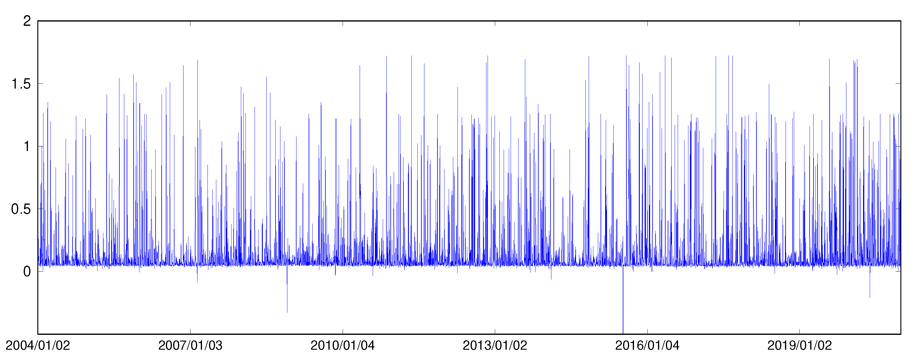
Figure 1 plots daily returns and logarithmic realized volatility measures of DIS. Table 1 provides summary statistics for daily returns, two versions of RV and logRV measures of DIS, IBM, SPY and SKHY. As evident from the nonzero skewness values and large values of kurtosis, all four return series exhibit asymmetric and leptokurtic features. The skewness of all logRV series deviate from zero and their kurtosis5 values are all greater than 6.5, which clearly departs from a normality assumption. The summary statistics of logRV data are consistent with findings reported in Corsi et al. (2008).
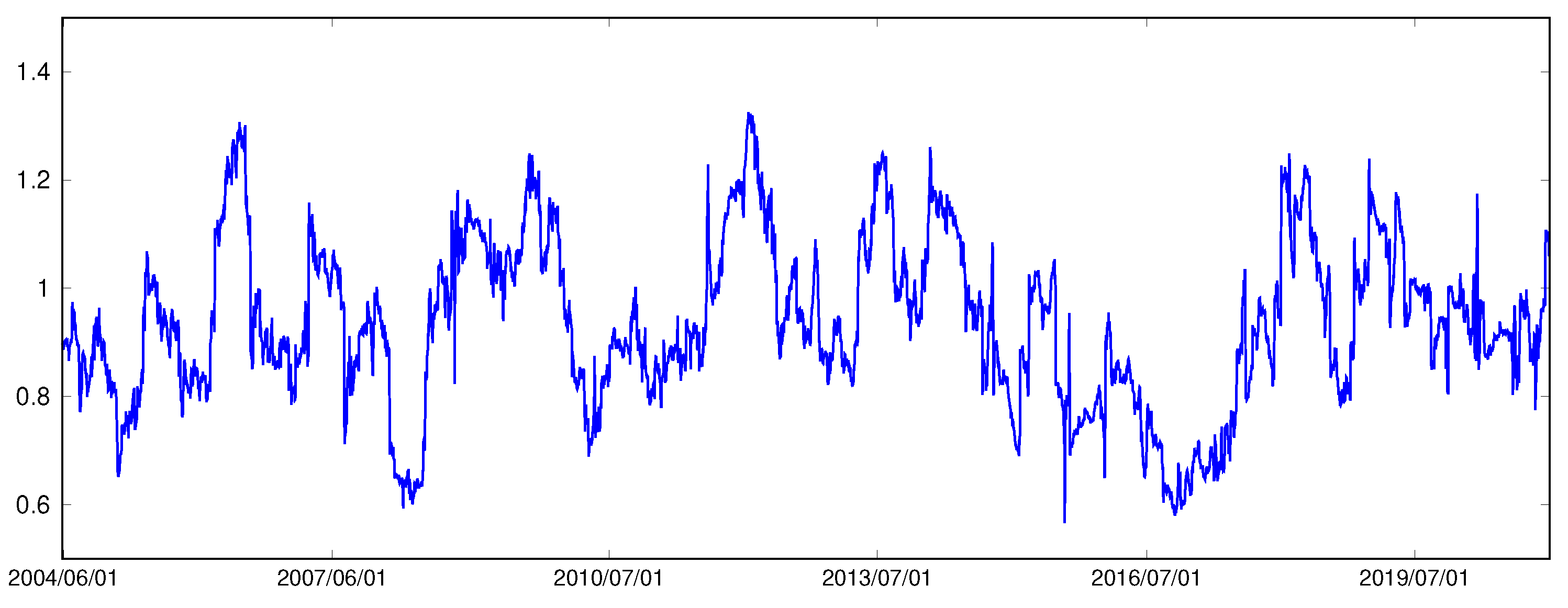
Volatility estimators such as SRV and RK are not bias-free, especially in finite samples. Table 1 shows that the two RV measures overestimate the return variance on average for DIS and IBM, but provide underestimations of SPY and SKHY return variance. However, the above results are based on the full sample and may not be true for subsamples. Figure 2 shows the ratios between the sample variance of returns and the sample mean of RV measures in 100-day rolling windows based on DIS. The ratio fluctuates between 0.57 and 1.33. Similarly, the ratio varies from 0.68 to 1.65 in the SPY case. The varying ratios suggest that the gap between return variance and RV average is not a constant and that RV estimation bias could be time-varying or state-dependent.
3. Models
3.1. Semiparametric Realized Stochastic Volatility Models
Following Jensen and Maheu (2010), I adopt the flexible distributional framework offered by the DPM and integrate it with the RSV model. The Gaussian innovation distributions for returns and logRV in the RSV model are replaced with nonparametric mixtures. In addition, the RV bias correction term is assumed to follow the DPM to more flexibly adjust the RV estimation bias. DPM is a nonparametric version of the finite mixture model. Unlike the conventional mixture, which requires a predetermined number of distributions, DPM allows the number of clusters to be nonfixed and learned endogenously from the data. Such a flexible framework is achieved with the use of the Dirichlet process (DP) formally introduced by Ferguson (1973). The DP is an infinite-dimensional generalization of the Dirichlet distribution and can be seen as a distribution of distributions. Let G represent a discrete distribution for mixture parameters. Imposing as a prior for G makes the number of clusters and the corresponding weights in G random. in is the concentration parameter that influences the likelihood of creating new clusters. The larger the value of is, the more mixtures the DPM contains. is the base function for DP and serves as the center of G.
Expressing the DP prior as the stick-breaking form by Sethuraman (1994), the RSV model incorporated with DPM (RSV-DPM) is given as
The return and logRV are linked by the latent log volatility , which follows the parametric autoregressive process defined by Equation (9). Parameters , , and are all state-dependent and follow the distribution G, whose prior is . As in Jensen and Maheu (2010), a mixture with state-dependent mean and volatility scalar is applied to fit the return innovation distribution. Parameters and in Equation (8) correspond to the RV estimation bias and logRV variance, respectively. Allowing and to be nonfixed not only accommodates the non-Gaussian features of logRV, but also allows flexible adjustment for RV bias. To maintain parsimony, I assume that all state-dependent parameters are governed by the underlying state variable . is the state probability vector whose elements are generated from the stick-breaking process in Equation (11). The DP prior’s base function is defined as , , and , where IG stands for an inverse-gamma distribution. The prior for is and . A hierarchical prior is placed on to add more flexibility.
I further consider an alternative semiparametric RSV model termed RSV-DPM-ind, which assigns two independent DPMs to return and logRV processes and analyzes logRV as follows.
Equations (7), (9)–(12) and (13)–(16) constitute the RSV-DPM-ind model. Underlying state variables and govern return and logRV, respectively. Parameters and follow the distribution H, whose prior is with base function and . The model settings for return and latent log volatility processes are the same as the RSV-DPM model, except that the DPM with prior only governs and .
In addition, a semiparametric RSV model with DPM influencing only the return process is included for the purpose of model comparison. Termed RSV-DPM-ret, the model is constituted by Equations (7) to (12) but with fixed parameters and in the logRV equation.
The first-order autoregressive latent volatility process can be generalized to include more lagged terms, factor capturing volatility-feedback effect, or additional predictors. For example, Huang et al. (2019) find that the option implied volatility (IV) benefits the prediction of future RV. Equation (9) could contain IV as an additional explanatory variable. In addition, motivated by Corsi et al. (2008), the realized quarticity (RQ), which measures the volatility of RV, can be potentially incorporated in Equation (8) to improve the characterization of the logRV residual error. All of those are left for future studies.
3.2. Benchmark Models
Several volatility models are considered as benchmarks. The first benchmark is the RSV model, which analyzes return and logRV in the following parametric way.
Combining Equations (9), (17) and (18) completes the RSV model. To evaluate the proposed models with existing semiparametric SV models, we consider the SV-DPM designed by Jensen and Maheu (2010). Equations (7), (9)–(12) constitute the SV-DPM model, which does not take the RV information into account. The conventional SV model formed by Equations (9) and (17) and the SV model with Student’s t-distributed innovation term6 are included. Finally, the GARCH model and GARCH with Student’s t-distributed innovation (GARCH-t) are included as benchmarks. The GARCH model is given as
3.3. Bayesian Inference
The semiparametric RSV models are estimated using the Markov chain Monte Carlo (MCMC) technique. Taking the RSV-DPM model as an example, the parameter set includes , , and latent volatility series . The slice sampling technique introduced by Walker (2007) and further developed by Kalli et al. (2011) is applied to facilitate model estimation in infinite state space. Conditional on a set of auxiliary variables , the infinite number of clusters is randomly truncated to a finite number K, which facilitates the use of Gibbs sampling or Metropolis-Hasting algorithms to estimate model parameters.
Let , and . After augmenting and , the joint posterior is proportional to
Each MCMC iteration contains the following sampling steps.
- 1.
- Sample model parameters and conditional on .Given conjugate priors, the conditional posterior distributions of , , , , , and can be easily derived. See the Appendix A for details. Model parameters are estimated by iteratively using Gibbs samplers as follows.
- (a).
- for .
- (b).
- for .
- (c).
- for .
- (d).
- for .
- (e).
- .
- (f).
- .
- 2.
- Sample latent volatility for .Latent volatility variables are sampled using the Metropolis-Hasting algorithm with a single move sampler. The conditional posterior of is given asThe proposal distribution for is derived from the conditional posterior following the approach in Kim et al. (1998). We leave the details to the Appendix A. A proposed value is accepted with probability .
- 3.
- Sample state variable for from
- 4.
- Sample auxiliary variable for .
- (a).
- Calculate for , where is sampled from
- (b).
- Sampling for from .
- (c).
- Find the smallest K such that .
- 5.
- Sample based on K.Following the method proposed by Escobar and West (1994), is sampled from the Gamma mixture below.where and .
The estimation of the RSV-DPM-ind model is essentially the same as that of the RSV-DPM model but two sets of DPM-related parameters need to be estimated. The RSV-DPM-ret model shares the same estimation steps as RSV-DPM, except that and are sampled conditional on .
Posterior statistics can be calculated conditional on MCMC draws after dropping results in a burn-in period. For example, the posterior mean of based on G MCMC outputs is given as
where is the draw of . Similarly, the smoothed log volatility can be estimated as
3.4. Prediction
Since volatility is not observable but the return is, the density forecast of returns is a natural way to evaluate the predictive power of volatility models. The predictive likelihood for returns provides the measure of the density forecast and is defined as
For all semiparametric SV models, based on G MCMC outputs, can be obtained by integrating out parameter uncertainties as
where , and and are determined based on the predicted state . If , set and . If , and .
The log predictive likelihood () of model over the out-of-sample period from to T is
The model with a higher is preferred. In model comparison, it is convenient to compute the log predictive Bayes factor (). The between models and equals . A value greater than 5 suggests that strongly dominates . The subsample performance of density forecasts can be investigated using cumulative defined as follows.
For SV models incorporating RV measures, the predictive likelihood of logRV can be calculated similarly to evaluate the prediction of volatility measures.
Taking the RSV-DPM model as an example, can be consistently estimated based on posterior outputs as
where , . For state-dependent parameters, and if . and if .
4. Empirical Applications
This section reports the results of applying the proposed and benchmark models to the four data series discussed in Section 2. Model estimation is based on 5000 MCMC results, after 5000 burnin and the code is written in C programming language. The out-of-sample period starts on 2 January 2009, and contains 3021 days. We consider both SRV and RK discussed in Section 2 as volatility measures. The priors applied to the semiparametric RSV models are , , , for , for or 1, and . The benchmark models have the same priors for parameters , , , , and .
4.1. Parameter Estimates
Table 2 reports posterior estimates for the RSV-DPM, RSV-DPM-ind, RSV and SV-DPM models. Among the three models incorporating RV measures, the two semiparametric RSV models capture stronger volatility persistence than the conventional RSV model. The posterior means of in the RSV-DPM model for DIS, IBM, SPY, and SKHY are all higher than 0.96, while the RSV model reports values of 0.861, 0.887, 0.940, and 0.933 in the four cases. The variance estimates of log volatility in the proposed models are lower than those in the benchmark RSV model. For example, in the DIS application, the posterior mean of in RSV-DPM is 0.0325, but the RSV model estimates as 0.1922. To mitigate the gap between return variance and RV, the RSV model uses a positive bias correction term for DIS and IBM and a negative for SPY and SKHY. The sign of is consistent with the relationship between return variance and RV averages observed in Table 1. The semiparametric RSV models, in contrast, adjust the estimation bias more flexibly via a time-varying correction term. Figure 3 plots from RSV-DPM model7 in the DIS case. is on average positive but varies substantially from large values to even negative values. In addition, the proposed models report lower posterior standard deviations of and than the RSV model, which suggests that the Bayesian nonparametric extension improves the precision of latent volatility parameter estimation. The results are based on ex-post volatility measured by SRV, and using RK leads to similar results.
A comparison of the estimation results of the three semiparametric models shows that the RSV-DPM-ind model requires fewer mixtures to fit the asymmetric and leptokurtic properties of returns, whereas the SV-DPM model has to rely on additional mixtures. For example, the mixture for return distributions in the RSV-DPM-ind model contains on average 3.05, 2.89, 1.88 and 2.15 Gaussian distributions in the four applications, whereas the average numbers of clusters in the SV-DPM model are 5.51, 3.56, 8.34, and 3.59.
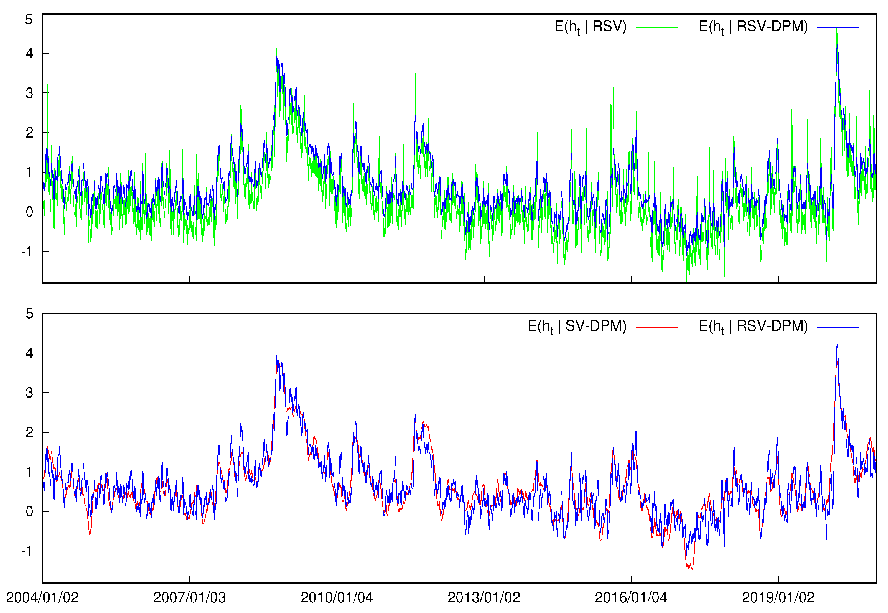
As shown in the top panel of Figure 4, the latent volatility estimates of the RSV model is noisier than that of the RSV-DPM model, which is consistent with the weaker volatility persistence and higher logRV volatility shown in Table 2. Such a result indicates that without non-Gaussian innovation terms, volatility fluctuates more to accommodate the return distribution, which sacrifices the time-dependent nature of volatility. The bottom panel of Figure 4 shows that the RSV-DPM model captures similar time-series volatility dynamics as the SV-DPM model.
4.2. Density Forecasts
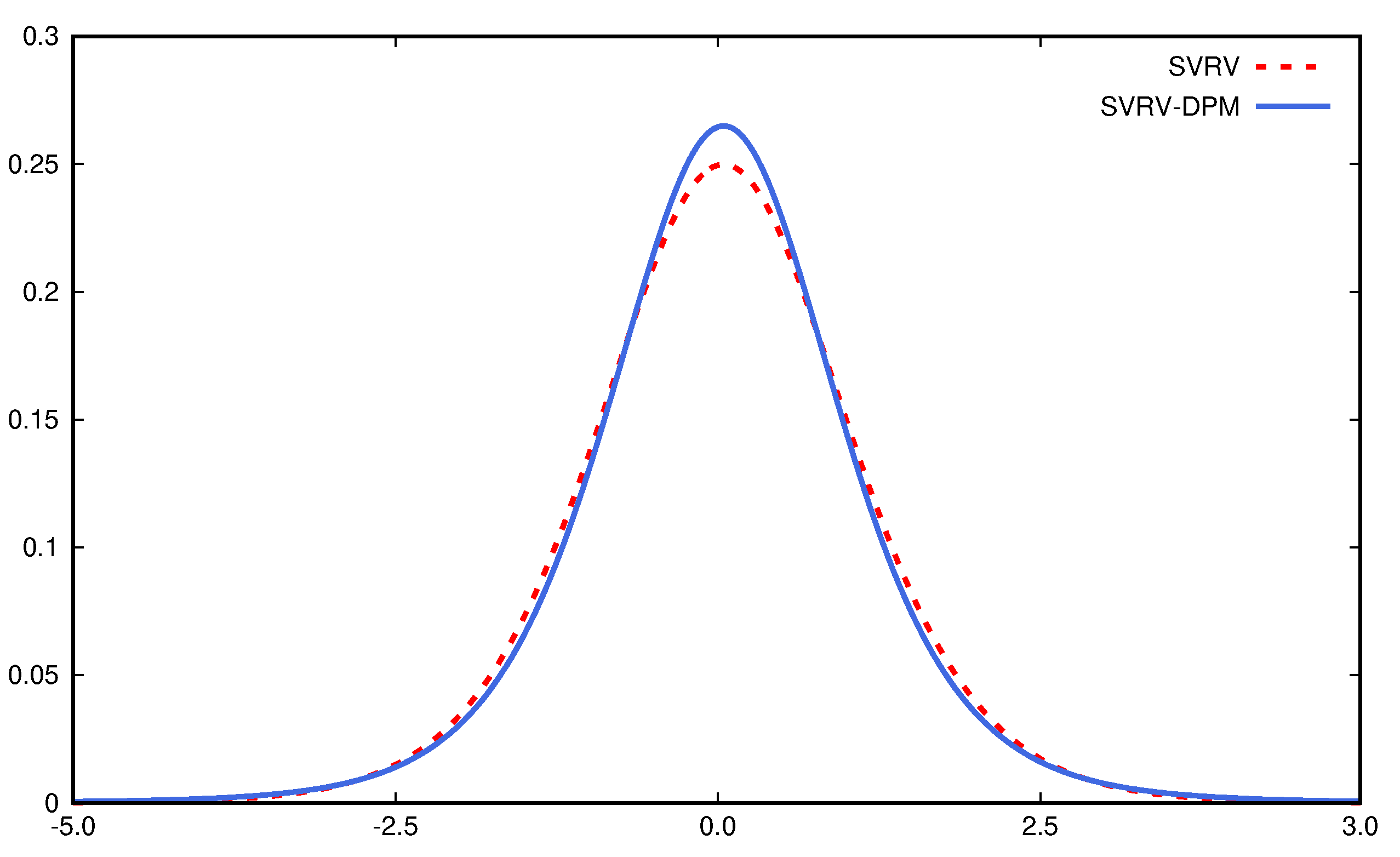
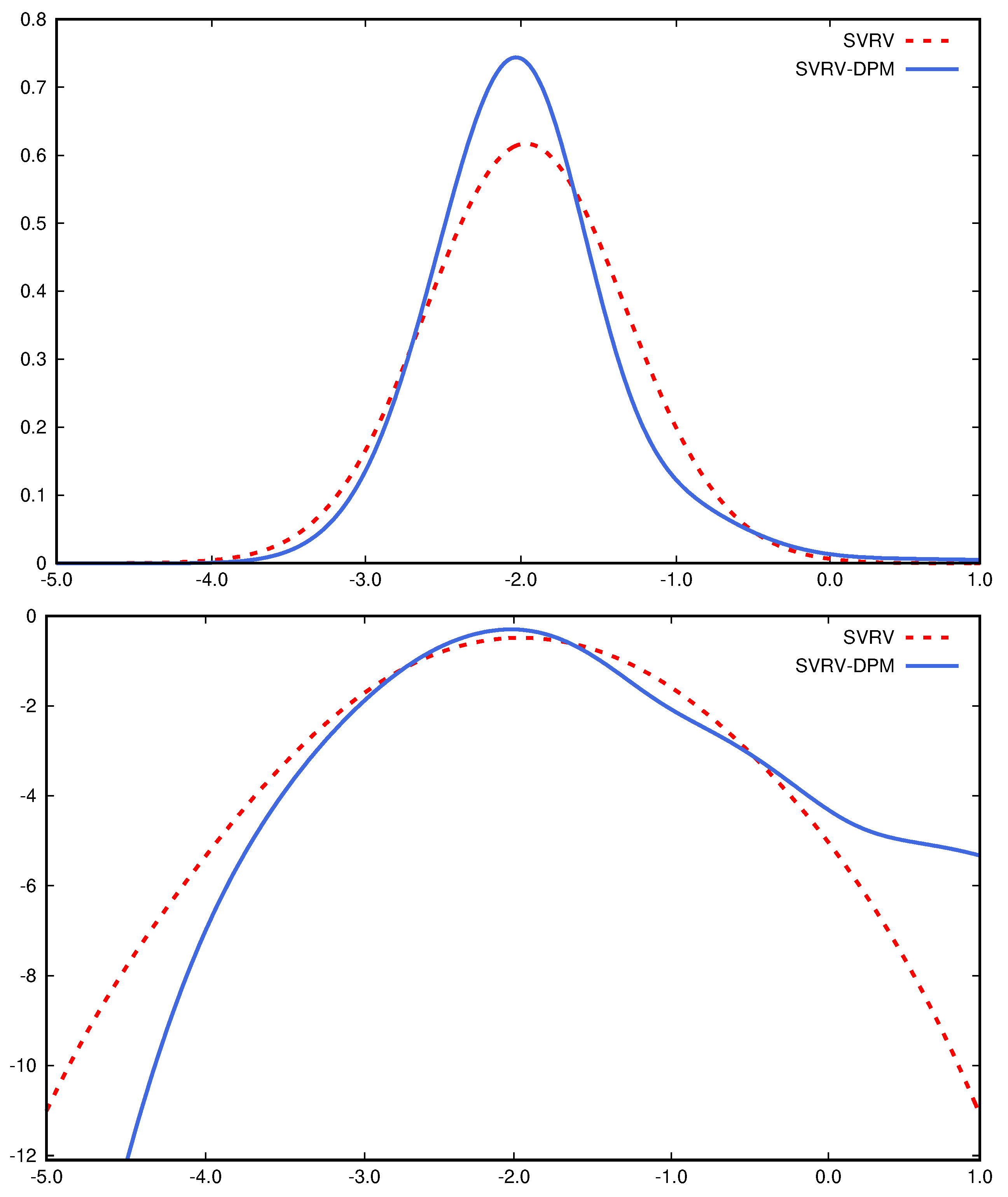
The top panel of Figure 5 plots the predictive return density of DIS on 31 December 2020, from the RSV and RSV-DPM models. The bottom panel of Figure 5 provides the log predictive density of returns to more clearly visualize the tail pattern. The predictive return density under the RSV-DPM model is asymmetric and heavy-tailed, in contrast to the Gaussian density under the RSV model. The predictive density of logRV and its log density can be found in Figure 6. The RSV-DPM model fits logRV using a skewed density with a heavy right tail, which is not achievable with the Gaussian assumption in the benchmark RSV model.
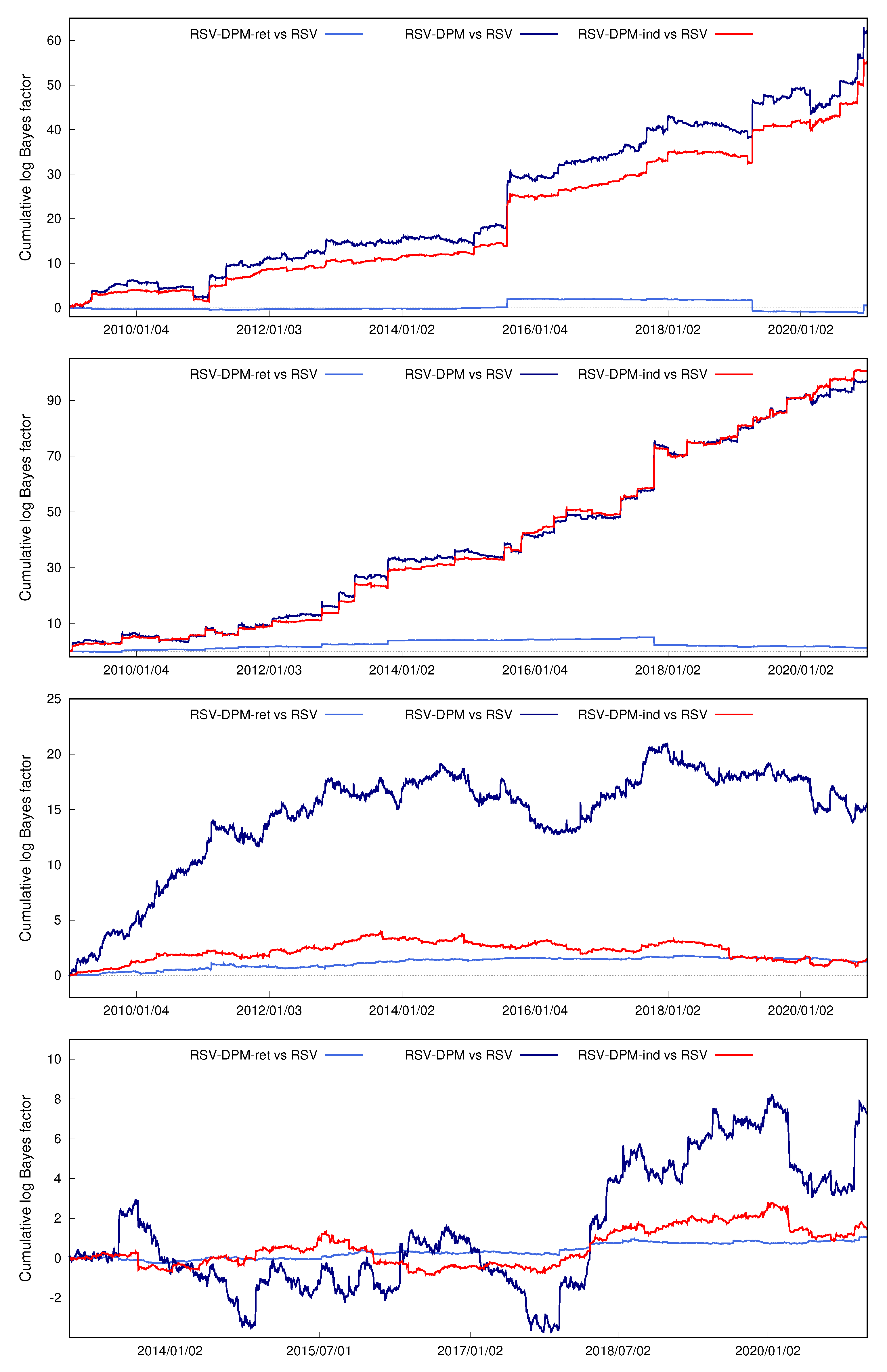
Table 3 reports the log predictive likelihoods of returns at three forecast horizons and log predictive Bayes factors against the SV model. In all four asset cases, either the semiparametric SV or RSV model outperforms the basic SV model in terms of return density forecasting. While the parametric RSV model fails to provide better density forecasts of DIS and IBM returns than the SV-DPM model, the semiparametric versions of the RSV model improve return density forecasts significantly in all four asset cases, compared with the benchmarks. For example, based on SRV measures, the log predictive Bayes factors of RSV-DPM relative to RSV are 60.8, 96.5, 16.8, and 7.3 in DIS, IBM, SPY, and SKHY applications, respectively. Density forecasts of DIS, SPY, and SKHY returns suggest that RSV-DPM is the top-performing model, and the IBM result favors the RSV-DPM-ind model slightly more. The log predictive Bayes factors between the RSV-DPM and RSV model in DIS and IBM cases are larger than those in the other two cases, which suggests the proposed extension offers more improvement when logRV data is more skewed and has heavier tails. The RSV-DPM-ret model, which only extends the return innovation distribution to DPM, provides very small forecast improvements compared with the benchmark RSV model. The results among the three semiparametric RSV models show that the relaxation of assumptions about logRV distribution and RV bias are the main drivers for improving return density forecasts. The upward slope cumulative log predictive Bayes factors shown in Figure 7 confirm that the RSV-DPM model consistently offers density forecast improvement over the RSV model in subsample periods. Table 3 also shows that the proposed models have improved density forecasts of returns over five and ten days in most of the cases considered and the ranking of models is robust to the choice of RV measures.
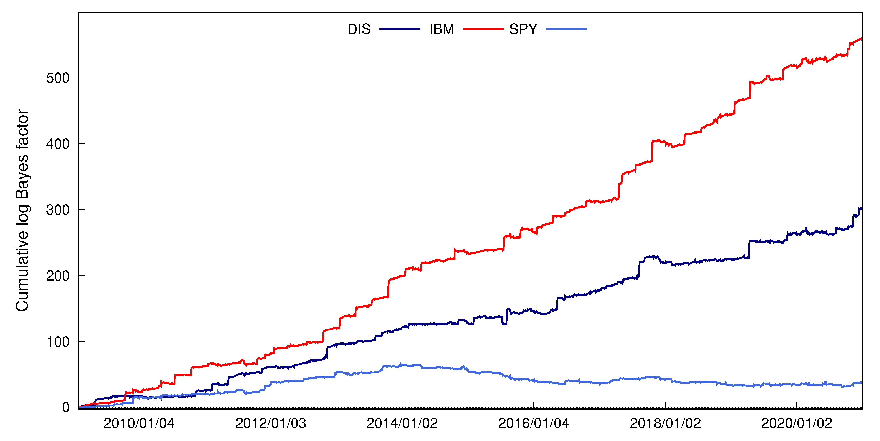
Table 4 summarizes the results of the density forecast of logRV in the four asset applications. The RSV-DPM and RSV-DPM-ind models offer more accurate logRV density forecasts than the benchmark RSV model. The one-period ahead log predictive likelihoods of both RSV-DPM and RSV-DPM-ind are 300, 500, 30 and 90 units higher than the RSV model in the DIS, IBM, SPY and SKHY cases, respectively. The cumulative log predictive Bayes factors shown in Figure 8 confirm that the logRV density forecast results are robust to subsamples. The RSV-DPM-ind model, which assumes returns and logRV is governed by two independent DPMs, offers the best one-period ahead density forecast of logRV. The more parsimonious RSV-DPM model yields better density forecasts of logRVs over longer periods.
5. Conclusions
This paper contributes to the SV modeling literature by integrating the RSV model with a Bayesian nonparametric framework. Such an extension benefits the volatility modeling in two aspects. First, the Bayesian nonparametric mixture better fits the empirical distributions of returns and logRVs, compared with Gaussian densities. Second, the information from high-frequency volatility measures can be better utilized by allowing more flexible RV bias adjustment.
Applications to DIS, IBM, SPY, and SKHY data compare the proposed model with benchmarks including RSV, SV-DPM, SV-t, SV, and GARCH. The semiparametric RSV model offers a significant improvement on density forecast of return and logRV, especially for asset data with more severe asymmetric and leptokurtic features. Compared with the parametric RSV model, the proposed model yields less noisy and more persistent latent volatility series.
The forecasting improvements mainly originate from the generalization of the logRV framework. The empirical results of this paper are consistent with Corsi et al. (2008) that non-Gaussian densities better characterize logRV. Another suggestion from this study is that RV estimation bias may not remain constant and it is beneficial to filter out the time-varying bias flexibly. One potential future research direction is to adopt a time-dependent mixture, so that the volatility of logRV and bias adjustment parameter is related to past values and allowed to cluster. Another area of potential research is to explore if the information from realized quarticity could be incorporated to improve the characterization of the volatility of logRV.
Funding
This research received no external funding.
Institutional Review Board Statement
Not applicable.
Informed Consent Statement
Not applicable.
Data Availability Statement
The data presented in this study are obtained from Tick Data (https://www.tickdata.com/ accessed on 15 August 2021).
Conflicts of Interest
The author declares no conflict of interest.
Appendix A
The estimation for parameters in the RSV-DPM model contains the following steps.
- 1.
- for .Given prior , the conditional posterior of is given aswhere
- 2.
- .Given prior , the conditional posterior of is given aswhere .
- 3.
- Given prior , the conditional posterior of is given aswhere
- 4.
- Given prior , the conditional posterior of is given as
- 5.
- Let , and , where . Given prior , the conditional posterior of is given aswhere
- 6.
- Given prior , the conditional posterior of is given as
- 7.
- for .The conditional posterior of is given aswhereandKim et al. (1998) show thatwhereand is the proposal distribution for drawing . A new value is accepted with probability .
| 1 | Under the previous-tick scheme, is the price observed the nearest before time . |
| 2 | The Parzen kernel function is given as
|
| 3 | is calculated using high-frequency returns such as every q trades, and is the number of nonzero returns. I set . |
| 4 | https://www.tickdata.com/, accessed on 15 August 2021. |
| 5 | The kurtosis measure is calculated using formula . |
| 6 | The innovation term , where is the degree of freedom. |
| 7 | To better visualize the bias correction difference in RSV-DPM and RSV models, we set the scaling parameter to be 1 to make two models have the same setting in return variance. |
References
- Andersen, Torben G., Tim Bollerslev, Francis X. Diebold, and Heiko Ebens. 2001. The distribution of realized stock return volatility. Journal of Financial Economics 61: 43–76. [Google Scholar] [CrossRef]
- Asai, Manabu, Chia-Lin Chang, and Michael McAleer. 2017. Realized stochastic volatility with general asymmetry and long memory. Journal of Econometrics 199: 202–12. [Google Scholar] [CrossRef] [Green Version]
- Bandi, Federico M., and Jeffrey R. Russell. 2008. Microstructure noise, realized variance, and optimal sampling. The Review of Economic Studies 75: 339–69. [Google Scholar] [CrossRef]
- Bandi, Federico M., Jeffrey R. Russell, and Chen Yang. 2013. Realized volatility forecasting in the presence of time-varying noise. Journal of Business & Economic Statistics 31: 331–45. [Google Scholar]
- Barndorff-Nielsen, Ole E. 1997. Normal inverse gaussian distributions and stochastic volatility modelling. Scandinavian Journal of Statistics 24: 1–13. [Google Scholar] [CrossRef]
- Barndorff-Nielsen, Ole E., and Neil Shephard. 2002. Estimating quadratic variation using realized variance. Journal of Applied Econometrics 17: 457–77. [Google Scholar] [CrossRef] [Green Version]
- Barndorff-Nielsen, Ole E., and Neil Shephard. 2004. Power and Bipower Variation with Stochastic Volatility and Jumps. Journal of Financial Econometrics 2: 1–37. [Google Scholar] [CrossRef] [Green Version]
- Barndorff-Nielsen, Ole E., Peter Reinhard Hansen, Asger Lunde, and Neil Shephard. 2008. Designing realized kernels to measure the ex post variation of equity prices in the presence of noise. Econometrica 76: 1481–536. [Google Scholar]
- Barndorff-Nielsen, Ole E., Peter Reinhard Hansen, Asger Lunde, and Neil Shephard. 2009. Realized kernels in practice: Trades and quotes. Econometrics Journal 12: C1–C32. [Google Scholar] [CrossRef]
- Bollerslev, Tim. 1986. Generalized autoregressive conditional heteroskedasticity. Journal of Econometrics 31: 307–27. [Google Scholar] [CrossRef] [Green Version]
- Chib, Siddhartha, Federico Nardari, and Neil Shephard. 2002. Markov chain monte carlo methods for stochastic volatility models. Journal of Econometrics 108: 281–316. [Google Scholar] [CrossRef]
- Christensen, Kim, and Mark Podolskij. 2007. Realized range-based estimation of integrated variance. Journal of Econometrics 141: 323–49. [Google Scholar] [CrossRef]
- Corsi, Fulvio, Stefan Mittnik, Christian Pigorsch, and Uta Pigorsch. 2008. The volatility of realized volatility. Econometric Reviews 27: 46–78. [Google Scholar] [CrossRef]
- Delatola, Eleni-Ioanna, and Jim E. Griffin. 2013. A bayesian semiparametric model for volatility with a leverage effect. Computational Statistics & Data Analysis 60: 97–110. [Google Scholar]
- Escobar, Michael D., and Mike West. 1994. Bayesian Density Estimation and Inference Using Mixtures. Journal of the American Statistical Association 90: 577–88. [Google Scholar] [CrossRef]
- Ferguson, Thomas S. 1973. A Bayesian analysis of some nonparametric problems. The Annals of Statistics 1: 209–30. [Google Scholar] [CrossRef]
- Hansen, Peter Reinhard, and Asger Lunde. 2005. A Realized Variance for the Whole Day Based on Intermittent High-Frequency Data. Journal of Financial Econometrics 3: 525–54. [Google Scholar] [CrossRef]
- Hansen, Peter Reinhard, Zhuo Huang, and Howard Howan Shek. 2012. Realized garch: A joint model for returns and realized measures of volatility. Journal of Applied Econometrics 27: 877–906. [Google Scholar] [CrossRef]
- Huang, Darien, Christian Schlag, Ivan Shaliastovich, and Julian Thimme. 2019. Volatility-of-volatility risk. Journal of Financial and Quantitative Analysis 54: 2423–52. [Google Scholar] [CrossRef] [Green Version]
- Jacod, Jean, Yingying Li, Per A. Mykland, Mark Podolskij, and Mathias Vetter. 2009. Microstructure noise in the continuous case: The pre-averaging approach. Stochastic Processes and their Applications 119: 2249–76. [Google Scholar] [CrossRef] [Green Version]
- Jensen, Mark J., and John M. Maheu. 2010. Bayesian semiparametric stochastic volatility modeling. Journal of Econometrics 157: 306–16. [Google Scholar] [CrossRef] [Green Version]
- Jensen, Mark J., and John M. Maheu. 2014. Estimating a semiparametric asymmetric stochastic volatility model with a dirichlet process mixture. Journal of Econometrics 178: 523–38. [Google Scholar] [CrossRef] [Green Version]
- Kalli, Maria, Jim E. Griffin, and Stephen G. Walker. 2011. Slice sampling mixture models. Statistics and Computing 21: 93–105. [Google Scholar] [CrossRef]
- Kim, Sangjoon, Neil Shephard, and Siddhartha Chib. 1998. Stochastic volatility: Likelihood inference and comparison with arch models. The Review of Economic Studies 65: 361–93. [Google Scholar] [CrossRef]
- Liu, Jia, and John M. Maheu. 2018. Improving markov switching models using realized variance. Journal of Applied Econometrics 33: 297–318. [Google Scholar] [CrossRef] [Green Version]
- Maheu, John, and Thomas McCurdy. 2011. Do high-freuqency measures of volatility improve forecasts of returns distributions? Journal of Econometrics 160: 69–76. [Google Scholar] [CrossRef] [Green Version]
- Mahieu, Ronald, and Peter C. Schotman. 1998. An empirical application of stochastic volatility models. Journal of Applied Econometrics 13: 333–60. [Google Scholar] [CrossRef] [Green Version]
- Nakajima, Jouchi, and Yasuhiro Omori. 2012. Stochastic volatility model with leverage and asymmetrically heavy-tailed error using gh skew student’s t-distribution. Computational Statistics & Data Analysis 56: 3690–704. [Google Scholar]
- Sandmann, Gleb, and Siem Jan Koopman. 1998. Estimation of stochastic volatility models via monte carlo maximum likelihood. Journal of Econometrics 87: 271–301. [Google Scholar] [CrossRef]
- Sethuraman, Jayaram. 1994. A constructive definition of Dirichlet priors. Statistica Sinica 4: 639–50. [Google Scholar]
- Shephard, Neil, and Kevin Sheppard. 2010. Realising the future: Forecasting with high-frequency-based volatility (heavy) models. Journal of Applied Econometrics 25: 197–231. [Google Scholar] [CrossRef] [Green Version]
- Shirota, Shinichiro, Takayuki Hizu, and Yasuhiro Omori. 2014. Realized stochastic volatility with leverage and long memory. Computational Statistics and Data Analysis 76: 618–41. [Google Scholar] [CrossRef] [Green Version]
- Takahashi, Makoto, Yasuhiro Omori, and Toshiaki Watanabe. 2009. Estimating stochastic volatility models using daily returns and realized volatility simultaneously. Computational Statistics & Data Analysis 53: 2404–26. [Google Scholar]
- Taylor, Stephen J. 1986. Modelling Financial Time Series. Chichester: John Wiley. [Google Scholar]
- Virbickaitė, Audronė, and Hedibert F. Lopes. 2019. Bayesian semiparametric markov switching stochastic volatility model. Applied Stochastic Models in Business and Industry 35: 978–97. [Google Scholar] [CrossRef]
- Walker, Stephen G. 2007. Sampling the Dirichlet mixture model with slices. Communications in Statistics—Simulation and Computation 36: 45–54. [Google Scholar] [CrossRef]
- Xiu, Dacheng. 2010. Quasi-maximum likelihood estimation of volatility with high frequency data. Journal of Econometrics 159: 235–50. [Google Scholar] [CrossRef]
- Yu, Jun. 2012. A semiparametric stochastic volatility model. Journal of Econometrics 167: 473–82. [Google Scholar] [CrossRef]
- Zhang, Lan, Per A. Mykland, and Yacine Aït-Sahalia. 2005. A tale of two time scales: Determining integrated volatility with noisy high-frequency data. Journal of the American Statistical Association 100: 1394–411. [Google Scholar] [CrossRef]
Figure 1.
Daily returns and logarithmic realized volatility measures of DIS.

Figure 2.
Ratios between return variance and RV average of DIS in 100-days rolling window.

Figure 3.
Posterior mean of of DIS from the RSV-DPM model.

Figure 4.
Posterior mean of log volatilities of DIS.

Figure 5.
(Top): predictive return density ; (Bottom): log predictive return density of the RSV-DPM and RSV models.
Figure 5.
(Top): predictive return density ; (Bottom): log predictive return density of the RSV-DPM and RSV models.


Figure 6.
(Top): Predictive logRV density ; (Bottom): Log predictive logRV density of the RSV-DPM and RSV models.
Figure 6.
(Top): Predictive logRV density ; (Bottom): Log predictive logRV density of the RSV-DPM and RSV models.

Figure 7.
Cumulative log predictive Bayes factors for semiparametric RSV models vs the RSV model (from top to bottom: DIS, IBM, SPY and SKHY).
Figure 7.
Cumulative log predictive Bayes factors for semiparametric RSV models vs the RSV model (from top to bottom: DIS, IBM, SPY and SKHY).

Figure 8.
Cumulative log predictive Bayes factors for logRV between RSV-DPM and RSV models .


Table 1.
Descriptive statistics for returns and volatility measures of DIS, IBM, SPY and SKHY.
| Data | Mean | St. Dev. | Skewness | Kurtosis | Min | Max | |
|---|---|---|---|---|---|---|---|
| Panel A: DIS | |||||||
| 0.048 | 0.045 | 2.922 | 0.378 | 17.063 | −13.908 | 14.818 | |
| 3.022 | 1.255 | 74.446 | 12.149 | 214.107 | 0.101 | 222.816 | |
| 3.076 | 1.281 | 80.633 | 12.779 | 234.898 | 0.124 | 222.505 | |
| 0.372 | 0.227 | 0.982 | 1.023 | 7.823 | −2.296 | 5.406 | |
| 0.401 | 0.248 | 0.943 | 1.100 | 8.026 | −2.089 | 5.405 | |
| Panel B: IBM | |||||||
| 0.007 | 0.025 | 2.055 | −0.378 | 14.591 | −13.755 | 10.899 | |
| 2.232 | 0.952 | 34.375 | 9.621 | 142.584 | 0.096 | 138.501 | |
| 2.296 | 0.969 | 36.599 | 9.258 | 126.467 | 0.113 | 128.970 | |
| 0.094 | −0.049 | 0.911 | 1.207 | 8.340 | −2.340 | 4.931 | |
| 0.125 | −0.032 | 0.890 | 1.284 | 8.555 | −2.180 | 4.860 | |
| Panel C: SPY | |||||||
| 0.028 | 0.065 | 1.476 | −0.389 | 21.891 | −11.589 | 13.558 | |
| 1.377 | 0.457 | 22.279 | 15.417 | 352.039 | 0.013 | 148.459 | |
| 1.405 | 0.466 | 22.680 | 15.250 | 343.385 | 0.017 | 147.030 | |
| −0.630 | −0.782 | 1.367 | 0.713 | 7.048 | −4.305 | 5.000 | |
| −0.595 | −0.764 | 1.331 | 0.757 | 7.104 | −4.079 | 4.991 | |
| Panel D: SKHY | |||||||
| 0.097 | 0.000 | 6.586 | 0.237 | 5.504 | −13.062 | 13.958 | |
| 6.559 | 4.348 | 54.981 | 4.240 | 28.222 | 0.589 | 87.957 | |
| 6.294 | 4.071 | 55.954 | 4.165 | 26.820 | 0.338 | 85.496 | |
| 1.559 | 1.470 | 0.536 | 0.727 | 6.758 | −0.529 | 4.477 | |
| 1.481 | 1.404 | 0.606 | 0.616 | 6.690 | −1.084 | 4.448 | |
This table reports the summary statistics of daily returns (rt), subsampled realized variance (SRVt),
realized kernel (RKt) and log volatility measures of DIS, IBM, SPY and SKHY.
Table 2.
Posterior estimates of the RSV-DPM, RSV-DPM-ind, RSV and SV-DPM models.
| RSV-DPM | RSV-DPM-ind | RSV | SV-DPM | |||||
|---|---|---|---|---|---|---|---|---|
| Mean | St. Dev. | Mean | St. Dev. | Mean | St. Dev. | Mean | St. Dev. | |
| Panel A: DIS | ||||||||
| 0.0480 | 0.0139 | |||||||
| 0.0538 | 0.0240 | |||||||
| 0.1934 | 0.0124 | |||||||
| 0.0120 | 0.0042 | 0.0607 | 0.0139 | 0.0055 | 0.0074 | 0.0023 | 0.0039 | |
| 0.9711 | 0.0041 | 0.9424 | 0.0072 | 0.8615 | 0.0147 | 0.9704 | 0.0057 | |
| 0.0325 | 0.0026 | 0.0816 | 0.0080 | 0.1922 | 0.0192 | 0.0461 | 0.0095 | |
| K | 6.2806 | 1.3239 | 3.0540 | 1.0079 | 5.5072 | 1.4271 | ||
| 0.4478 | 0.1878 | 0.2448 | 0.1379 | 0.3975 | 0.1857 | |||
| 3.9734 | 1.1658 | |||||||
| 0.2988 | 0.1567 | |||||||
| Panel B: IBM | ||||||||
| 0.0688 | 0.0154 | |||||||
| 0.0525 | 0.0240 | |||||||
| 0.1763 | 0.0102 | |||||||
| 0.0275 | 0.0056 | 0.0446 | 0.0085 | 0.0360 | 0.0075 | 0.0132 | 0.0042 | |
| 0.9662 | 0.0049 | 0.9553 | 0.0058 | 0.8866 | 0.0112 | 0.9795 | 0.0043 | |
| 0.0446 | 0.0042 | 0.0535 | 0.0049 | 0.1776 | 0.0152 | 0.0324 | 0.0053 | |
| K | 5.1318 | 1.1947 | 2.8922 | 1.2027 | 3.5662 | 1.4451 | ||
| 0.3797 | 0.1758 | 0.2363 | 0.1413 | 0.2747 | 0.1576 | |||
| 5.2840 | 2.0734 | |||||||
| 0.3817 | 0.2005 | |||||||
| Panel C: SPY | ||||||||
| 0.0937 | 0.0094 | |||||||
| −0.0808 | 0.0230 | |||||||
| 0.2176 | 0.0088 | |||||||
| −0.0337 | 0.0067 | −0.0484 | 0.0124 | −0.0328 | 0.0068 | −0.0177 | 0.0057 | |
| 0.9667 | 0.0045 | 0.9429 | 0.0066 | 0.9405 | 0.0065 | 0.9793 | 0.0040 | |
| 0.0707 | 0.0056 | 0.1300 | 0.0106 | 0.1357 | 0.0101 | 0.0689 | 0.0090 | |
| K | 5.1950 | 1.2383 | 1.8864 | 0.9991 | 8.3496 | 3.5307 | ||
| 0.3769 | 0.1723 | 0.1746 | 0.1214 | 0.5806 | 0.2952 | |||
| 3.1826 | 1.1761 | |||||||
| 0.2532 | 0.1422 | |||||||
| Panel D: SKHY | ||||||||
| 0.0885 | 0.0384 | |||||||
| −0.0566 | 0.0308 | |||||||
| 0.2068 | 0.0077 | |||||||
| 0.0459 | 0.0087 | 0.0830 | 0.0139 | 0.1074 | 0.0157 | 0.0165 | 0.0053 | |
| 0.9688 | 0.0056 | 0.9473 | 0.0083 | 0.9331 | 0.0096 | 0.9676 | 0.0071 | |
| 0.0175 | 0.0022 | 0.0328 | 0.0043 | 0.0434 | 0.0055 | 0.0199 | 0.0039 | |
| K | 5.9140 | 1.0316 | 2.1472 | 1.2665 | 3.5878 | 1.4628 | ||
| 0.4347 | 0.1782 | 0.1937 | 0.1339 | 0.2848 | 0.1637 | |||
| 3.3990 | 1.3635 | |||||||
| 0.2701 | 0.1531 | |||||||
This table reports the posterior means and standard deviations of model parameters in the DIS, IBM
SPY and SKHY applications.
Table 3.
Return density forecasts.
| Panel A: DIS | ||||||
| SV | −5174.3 | −5194.5 | −5209.1 | |||
| SV-t | −5129.4 | 44.9 | −5157.6 | 36.9 | −5175.1 | 33.9 |
| GARCH | −5383.1 | −208.8 | −5333.2 | −138.7 | −5339.8 | −130.8 |
| GARCH-t | −5149.5 | 24.8 | −5177.0 | 17.6 | −5189.3 | 19.7 |
| SV-DPM | −5121.1 | 53.2 | −5150.5 | 44.0 | −5174.1 | 35.0 |
| RSV (SRV) | −5128.8 | 45.5 | −5185.9 | 8.6 | −5238.6 | −29.5 |
| RSV (RK) | −5140.4 | 33.9 | −5188.8 | 5.7 | −5235.8 | −26.7 |
| RSV-DPM-ret (SRV) | −5128.3 | 46.1 | −5184.9 | 9.6 | −5237.7 | −28.7 |
| RSV-DPM-ret (RK) | −5138.7 | 35.6 | −5189.1 | 5.4 | −5234.2 | −25.2 |
| RSV-DPM (SRV) | −5066.8 | 107.5 | −5142.6 | 51.9 | −5185.3 | 23.7 |
| RSV-DPM (RK) | −5070.2 | 104.1 | −5141.4 | 53.1 | −5185.5 | 23.5 |
| RSV-DPM-ind (SRV) | −5073.9 | 100.4 | −5150.9 | 43.6 | −5195.5 | 13.5 |
| RSV-DPM-ind (RK) | −5075.1 | 99.2 | −5152.0 | 42.5 | −5196.7 | 12.3 |
| Panel B: IBM | ||||||
| SV | −4851.8 | −4872.9 | −4894.2 | |||
| SV-t | −4797.7 | 54.1 | −4832.9 | 40.0 | −4860.6 | 33.60 |
| GARCH | −5127.2 | −275.4 | −4993.1 | −120.2 | −5008.6 | −114.43 |
| GARCH-t | −4825.4 | 26.4 | −4851.7 | 21.2 | −4872.6 | 21.53 |
| SV-DPM | −4792.2 | 59.6 | −4834.0 | 38.8 | −4859.8 | 34.40 |
| RSV (SRV) | −4846.2 | 5.6 | −4880.3 | −7.4 | −4913.3 | −19.10 |
| RSV (RK) | −4841.5 | 10.3 | −4880.3 | −7.4 | −4903.5 | −9.30 |
| RSV-DPM-ret (SRV) | −4844.9 | 6.9 | −4881.6 | −8.7 | −4913.9 | −19.77 |
| RSV-DPM-ret (RK) | −4834.1 | 17.7 | −4878.2 | −5.3 | −4902.0 | −7.84 |
| RSV-DPM (SRV) | −4749.3 | 102.5 | −4812.7 | 60.1 | −4843.2 | 50.95 |
| RSV-DPM (RK) | −4744.9 | 106.8 | −4814.3 | 58.6 | −4845.9 | 48.22 |
| RSV-DPM-ind (SRV) | −4745.5 | 106.2 | −4815.2 | 57.7 | −4844.6 | 49.57 |
| RSV-DPM-ind (RK) | −4739.6 | 112.2 | −4816.5 | 56.4 | −4843.7 | 50.47 |
| Panel C: SPY | ||||||
| SV | −3855.2 | −3956.1 | −4016.2 | |||
| SV-t | −3867.8 | −12.6 | −3943.1 | 12.9 | −3998.0 | 18.1 |
| GARCH | −3975.8 | −120.6 | −4060.3 | −104.3 | −4126.5 | −110.4 |
| GARCH-t | −3851.5 | 3.7 | −3945.9 | 10.1 | −4011.1 | 5.1 |
| SV-DPM | −3843.2 | 12.0 | −3940.1 | 16.0 | −3996.7 | 19.5 |
| RSV (SRV) | −3767.6 | 87.6 | −3908.3 | 47.8 | −3981.1 | 35.1 |
| RSV (RK) | −3768.8 | 86.4 | −3910.0 | 46.0 | −3980.0 | 36.1 |
| RSV-DPM-ret (SRV) | −3766.4 | 88.8 | −3908.0 | 48.1 | −3980.0 | 36.2 |
| RSV-DPM-ret (RK) | −3767.8 | 87.4 | −3909.8 | 46.2 | −3979.1 | 37.0 |
| RSV-DPM (SRV) | −3752.2 | 103.0 | −3891.3 | 64.7 | −3970.7 | 45.5 |
| RSV-DPM (RK) | −3750.6 | 104.6 | −3893.4 | 62.6 | −3972.8 | 43.3 |
| RSV-DPM-ind (SRV) | −3766.2 | 89.0 | −3910.7 | 45.4 | −3980.6 | 35.5 |
| RSV-DPM-ind (RK) | −3766.7 | 88.5 | −3913.3 | 42.7 | −3981.0 | 35.1 |
| Panel D: SKHY | ||||||
| SV | −4308.1 | −4304.7 | −4297.7 | |||
| SV-t | −4320.9 | −12.7 | −4315.2 | −10.6 | −4312.3 | −14.6 |
| GARCH | −4509.3 | −201.2 | −4507.5 | −202.8 | −4509.8 | −212.0 |
| GARCH-t | −4303.2 | 4.9 | −4302.5 | 2.2 | −4302.2 | −4.5 |
| SV-DPM | −4305.0 | 3.1 | −4299.5 | 5.2 | −4293.9 | 3.9 |
| RSV (SRV) | −4290.6 | 17.5 | −4288.5 | 16.1 | −4287.8 | 9.9 |
| RSV (RK) | −4290.5 | 17.6 | −4289.6 | 15.1 | −4288.5 | 9.2 |
| RSV-DPM-ret (SRV) | −4289.5 | 18.6 | −4288.3 | 16.4 | −4287.5 | 10.3 |
| RSV-DPM-ret (RK) | −4290.4 | 17.7 | −4290.0 | 14.6 | −4288.9 | 8.8 |
| RSV-DPM (SRV) | −4283.4 | 24.8 | −4287.3 | 17.4 | −4285.7 | 12.1 |
| RSV-DPM (RK) | −4281.4 | 26.7 | −4290.5 | 14.2 | −4286.4 | 11.3 |
| RSV-DPM-ind (SRV) | −4289.1 | 19.0 | −4289.2 | 15.5 | −4286.4 | 11.3 |
| RSV-DPM-ind (RK) | −4289.7 | 18.4 | −4291.8 | 12.8 | −4287.7 | 10.1 |
This table reports the log predictive likelihood and log Bayes factors. Bold numbers indicate the highest values.
Table 4.
Density forecasts of log realized volatility measures.
| Panel A: DIS | ||||||
| RSV (SRV) | −3166.5 | −3634.7 | −3853.0 | |||
| RSV-DPM-ret (SRV) | −3159.4 | 7.1 | −3618.4 | 16.3 | −3853.4 | −0.5 |
| RSV-DPM (SRV) | −2864.9 | 301.6 | −3313.5 | 321.2 | −3476.9 | 376.0 |
| RSV-DPM-ind (SRV) | −2860.9 | 305.5 | −3346.6 | 288.1 | −3559.6 | 293.3 |
| RSV (RK) | −2985.0 | −3496.2 | −3738.4 | |||
| RSV-DPM-ret (RK) | −2981.8 | 3.2 | −3492.2 | 4.0 | −3735.5 | 2.9 |
| RSV-DPM (RK) | −2614.3 | 370.7 | −3146.6 | 349.6 | −3328.9 | 409.5 |
| RSV-DPM-ind (RK) | −2598.4 | 386.5 | −3170.7 | 325.5 | −3410.2 | 328.2 |
| Panel B: IBM | ||||||
| RSV (SRV) | −3306.9 | −3569.9 | −3784.9 | |||
| RSV-DPM-ret (SRV) | −3304.2 | 2.8 | −3570.1 | −0.2 | −3784.3 | 0.5 |
| RSV-DPM (SRV) | −2746.3 | 560.7 | −3123.1 | 446.8 | −3324.3 | 460.6 |
| RSV-DPM-ind (SRV) | −2748.6 | 558.4 | −3163.0 | 406.9 | −3368.1 | 416.7 |
| RSV (RK) | −3168.4 | −3464.7 | −3669.8 | |||
| RSV-DPM-ret (RK) | −3171.8 | −3.4 | −3461.3 | 3.4 | −3676.9 | −7.0 |
| RSV-DPM (RK) | −2536.9 | 631.5 | −2973.8 | 490.9 | −3201.6 | 468.2 |
| RSV-DPM-ind (RK) | −2526.7 | 641.8 | −3009.4 | 455.3 | −3248.1 | 421.7 |
| Panel C: SPY | ||||||
| RSV (SRV) | −3328.5 | −3846.6 | −4067.6 | |||
| RSV-DPM-ret (SRV) | −3327.4 | 1.1 | −3844.5 | 2.1 | −4071.4 | −3.8 |
| RSV-DPM (SRV) | −3289.9 | 38.6 | −3849.9 | −3.3 | −4031.5 | 36.1 |
| RSV-DPM-ind (SRV) | −3273.7 | 54.8 | −3817.2 | 29.5 | −4042.9 | 24.7 |
| RSV (RK) | −3187.8 | −3762.3 | −3996.4 | |||
| RSV-DPM-ret (RK) | −3187.6 | 0.2 | −3768.1 | −5.8 | −3987.6 | 8.8 |
| RSV-DPM (RK) | −3152.9 | 34.9 | −3742.2 | 20.1 | −3946.6 | 49.8 |
| RSV-DPM-ind (RK) | −3112.3 | 75.5 | −3713.9 | 48.4 | −3955.0 | 41.4 |
| Panel D: SKHY | ||||||
| RSV (SRV) | −1722.1 | −1874.3 | −1911.4 | |||
| RSV-DPM-ret (SRV) | −1722.3 | −0.2 | −1873.0 | 1.2 | −1911.0 | 0.4 |
| RSV-DPM (SRV) | −1632.2 | 90.0 | −1782.0 | 92.3 | −1836.5 | 74.8 |
| RSV-DPM-sep (SRV) | −1629.8 | 92.4 | −1810.1 | 64.2 | −1856.6 | 54.8 |
| RSV (RK) | −1857.5 | −2013.0 | −2052.1 | |||
| RSV-DPM-ret (RK) | −1857.7 | −0.2 | −2013.3 | −0.3 | −2054.5 | −2.4 |
| RSV-DPM (RK) | −1803.7 | 53.8 | −1962.2 | 50.8 | −2003.0 | 49.1 |
| RSV-DPM-ind (RK) | −1798.2 | 59.3 | −1975.9 | 37.1 | −2016.2 | 35.9 |
This table reports the log predictive likelihood and log Bayes factors of predicting logRV densities. Bold numbers indicate the highest values.
Publisher’s Note: MDPI stays neutral with regard to jurisdictional claims in published maps and institutional affiliations. |
© 2021 by the author. Licensee MDPI, Basel, Switzerland. This article is an open access article distributed under the terms and conditions of the Creative Commons Attribution (CC BY) license (https://creativecommons.org/licenses/by/4.0/).
Share and Cite
MDPI and ACS Style
Liu, J. A Bayesian Semiparametric Realized Stochastic Volatility Model. J. Risk Financial Manag. 2021, 14, 617. https://0-doi-org.brum.beds.ac.uk/10.3390/jrfm14120617
AMA Style
Liu J. A Bayesian Semiparametric Realized Stochastic Volatility Model. Journal of Risk and Financial Management. 2021; 14(12):617. https://0-doi-org.brum.beds.ac.uk/10.3390/jrfm14120617
Chicago/Turabian StyleLiu, Jia. 2021. "A Bayesian Semiparametric Realized Stochastic Volatility Model" Journal of Risk and Financial Management 14, no. 12: 617. https://0-doi-org.brum.beds.ac.uk/10.3390/jrfm14120617