Examining the Impact of Financial Development on Energy Production in Emerging Economies

Abstract

Global energy production has been on the rise for many years, and reliance on traditional sources of energy remains strong. The extraction and production of energy can serve as an important avenue of growth, particularly for developing economies. To undertake such capital intensive project requires significant investment, and, intuitively, a well-functioning domestic financial system would be expected to aid in the growth of such industries. We investigate the relationship between financial development and energy production for 15 emerging countries, over the period of 1995–2017. After establishing the presence of a unit root, based upon panel data methods, a cointegrating relationship between financial development and energy production is confirmed. The results of the fully modified ordinary least squares (FMOLS) estimation establish a long run relationship in 11 of 15 countries in the sample. Panel Granger causality results provide a link between energy production and foreign direct investment (FDI), while such a link is absent for domestic credit. Policymakers should understand that development of the energy sector can provide an incentive for foreign firms to invest in emerging economics.

1. Introduction

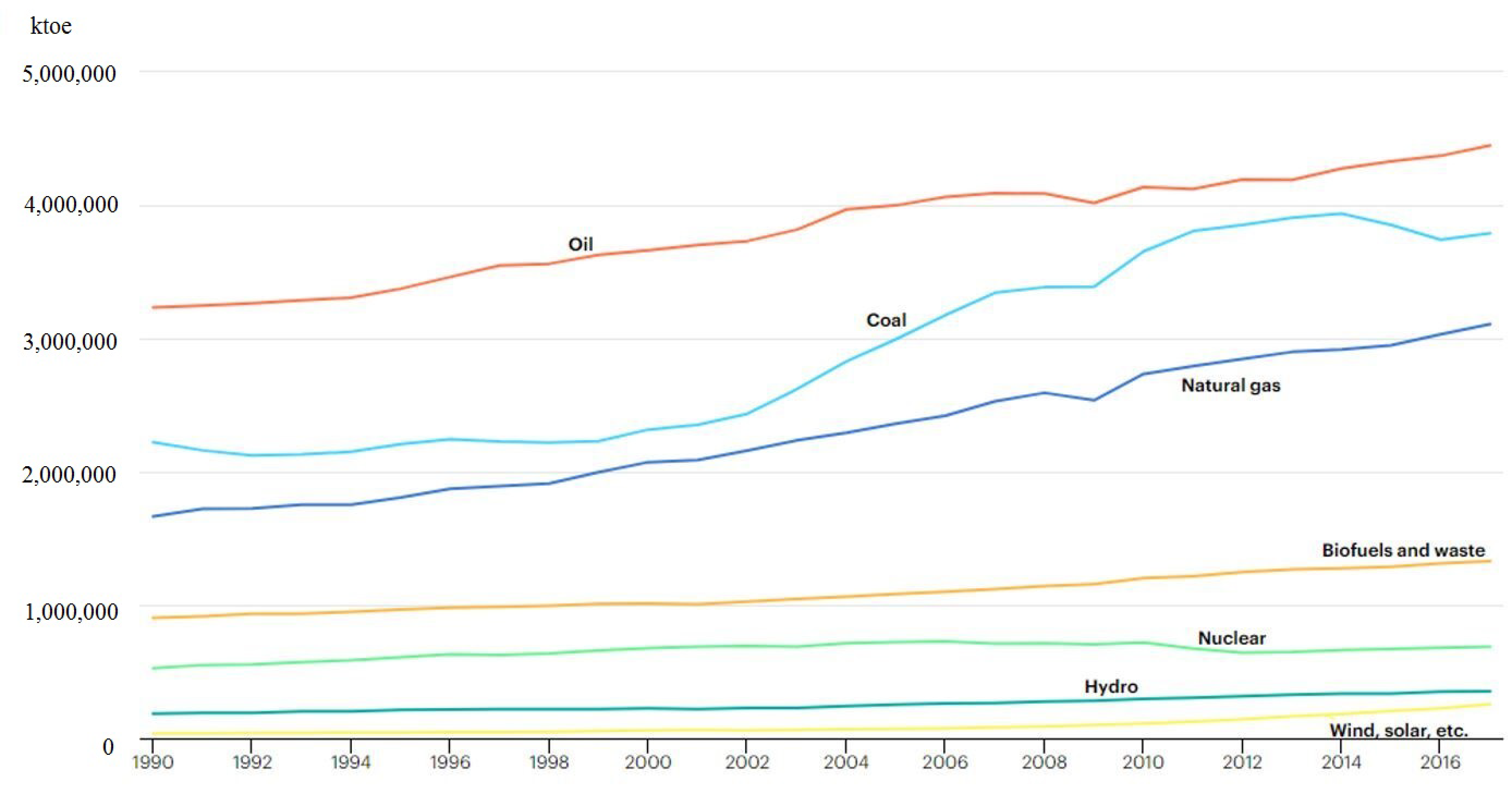
According to the International Energy Agency (2019), global Total Primary Energy Supply (TPES) has increased nearly 60% since 1990, to almost 14 million ktoe.1 While global energy production has been on the rise, the proportion of production which derives from conventional (fossil fuels) has remained relatively constant. In 1990, the share from fossil fuels was at 81%, where it remained in 2017. The distribution of the sources of energy over time is presented in Figure 1. The upward trend in both oil and natural gas are quite pronounced, while coal has recently experienced a decline from previous (record) high production. While much of the energy literature focus has been on renewable sources, technology, and the potential from such sources to positively impact the environment, it is clear that conventional sources remain the primary source of global energy.

The production of fossil fuel-based energy tends to be capital intensive, requiring significant levels of financing in order to bring production facilities online. A recent example in Kazakhstan highlights this fact. As discussed by Oil and Energy Trends (2019), the development of the giant Kashagan oil field required $50 billion (US) of investment, through 2017, leading to output of 300,000 bpd in 2018. Kazakhstan is notable for several reasons. First, according to the Energy Information Administration (EIA), it holds the twelfth largest reserves of oil in the world.2 Secondly, the central Asian country, which is an ex-Soviet Republic, is an emerging economy. As a new, open economy, Kazakhstan has attracted the attention and investment from major oil companies, including Chevron, Shell, and Total, along with Russia’s Lukoil and China’s CNPC and Sinopec.

Financing continues to be an important issue in the energy sector, both in terms of the required scale of funding and the need to allocate risks between both borrowers and lenders. Notably, the World Bank (2017) has recently taken a decision to end funding for upstream oil and gas projects (started in 2019). The bank defines upstream oil and gas as a term referring to exploration of oil and natural gas fields, and drilling and operating wells to produce oil and natural gas. This decision is based on the Bank’s commitments to accelerate the transitions to sustainable energy and support for the Paris Agreement goals. Future energy projects will require support from different sources, which are likely to include private capital. With fledgling intuitions and nascent financial markets, emerging economics that seek funding for energy projects would likely need to rely on foreign sources. From the investor’s point of view, a well-functioning financial domestic market, along with strong properties rights, should help temper country-specific risks of such investments. Contemporaneously, many emerging economies have experienced a dramatic change in economic institutions, particularly with respect to domestic financial sectors. The seminal work of North (1991) espouses the essential role of institutions to create efficient markets, which can then facilitate the growth of the economy. In the case of emerging economies, the comparative underdevelopment of these financial sectors could have implications on a country’s ability to provide the funding necessary to undertake the large-scale capital projects associated with primary energy production. Within this context, we investigate the potential relationship between financial development and energy production for 15 emerging economies. This sample of countries can be viewed in three separate subgroups: South/North American countries (Argentina, Brazil, Columbia, Mexico, and Uruguay), post-socialist countries (Mongolia, Poland, and Romania), and former Soviet republics including central Asian economies (Azerbaijan, Kazakhstan, and Kyrgyzstan) and others (Belarus, Georgia, Moldova, and Ukraine).

1.1. Former Soviet Republics

Almost three decades have passed since the collapse of the Soviet Union. The former Soviet republics differ greatly from one another in their political interest, the degree of economic integration and industrial cooperation, population, culture, and reserves of natural resources. These countries are divided into resource-rich and resource-poor. For example, Kazakhstan has significant reserves of oil and gas resources, whereas Kyrgyzstan has only water resource (Belousov and Vlasov 2010). One group of countries—the Central Asian Republics (CARs)—traditionally receives less attention. The CARs have a strategically important geographical location, land-locked between Asia and Europe, and are receiving an increasing interest recently from rapidly growing countries such as China. As part of the Soviets integrated production system, the CARs used to supply energy products, raw materials, and other intermediate products to Russia, while receiving manufactured products (Dowling and Wignaraja 2007). The CARs are rich with crude oil, natural gas, cotton, gold, copper, aluminum, and iron. These resource-rich countries have become heavily dependent on commodity exports as a source of revenue and domestic investment.

In the early years of transition, Kazakhstan, the largest of country in the CARs region, experienced an abrupt decline in oil production due to the loss of subsidies from Moscow and a lack of skilled professionals. Between 1997–2004, Kazakhstan and Azerbaijan have doubled their inflows of foreign direct investment(FDI). As a result, domestic oil, gas, and mining sectors have reaped significant benefits from the inflow of FDI, rather than domestic credits provided by banks.

The collapse of Soviet Union caused a major impact on the economic transition of the other former republics such as Belarus, Georgia, Ukraine, and Moldova. These countries faced many challenges including a lack of experienced management and administrative personnel, skilled labor, dependence on Russian energy, underdeveloped institutional and social infrastructure, and deep corruption. Even though Ukraine has a wealth of reserves of coal, oil, and gas, it remains heavily dependent on Russian energy resources and has had to pay above market prices on imported Russian gas (Ghedrovici and Ostapenko 2013). Recently, Ukraine announced a new policy, “Energy Strategy until 2030”, which sets the country’s energy priorities. This delayed response is primarily due to an individual groups’ moneyed interest in the Russian gas trade, inadequate governance, inability of social forces to establish equitable conditions for their citizens, and the tolerance of corruption.

With few energy resources, Moldova must import substantial amounts of fossil fuels to produce energy domestically. The country joined Europe’s Energy Community, although it still relies heavily on natural gas imports from Russia. Post-Soviet Belarus has remained firmly anti-capitalist, and strong links with Russia remain. Belarus has both crude oil and natural gas reserves, concentrated in the Pripyat basin (Energy Information Administration 2019), and the EIA expects that oil will account for nearly 80% of energy production in 2020.

1.2. Post-Socialist Countries

Poland, Romania, and Mongolia used to be members of the Council of Economic Cooperation during the Soviet era. In January 1990, the post-communist Polish government introduced the most radical economic reforms that had ever been undertaken in any country in 20th century. The goals of the Balcerowitcz plan, named after the finance minister at the time, included reducing the inflation rate, liberalization of prices and foreign international trade, elimination of food shortages, and flexible currency markets. Given its ample reserves of coal, Poland is heavily reliant on energy produced from fossil fuels. Given the relative size of its crude oil and natural gas reserves, Poland imports energy commodities from regional suppliers.

Romania abandoned the centrally planned economic model along with the corresponding political regime in December 1989 with the fall of Nicolae Ceausescu. The provisional government immediately began implementing economic reforms. The main sources of domestic energy production are coal and hydroelectric. Described as one the most energy-independent countries in Europe, according to Energy Information Administration (2015), Romania also possess one of the largest reserves of crude oil and shale gas in Europe.

After nearly 70 years, Mongolia abandoned their centrally planned economic system in 1991, and began its transition toward a market economy. The economic reform started with establishing a legal framework of free market economy, creating a two-tiered banking system, liberalizing the price level, and privatization of the state owned enterprises. GDP is now 12 times the level in 1990, leading the World Bank to classify Mongolia as a middle-income economy. Mongolia has significant coal reserves, and the vast majority of its energy production derives from coal.

1.3. South and Central America

The countries of the South American and Central American region have not endured the same transition as the previously discussed countries. Argentina has experienced rapid inflation and sovereign debt defaults, which has left the economy struggling. Argentina is the largest dry gas producer in South America and holds significant oil reserves, yet crude oil production is in decline due to a lack of investment (Energy Information Administration 2020). While Brazil as a democracy has experienced recent setbacks, it continues to be an important player in regional energy production. Brazil is the world’s 12th largest producer of oil, holds major natural gas reservoirs, and has the world’s second largest shale oil resources. Coal represents Columbia’s top mining export, while Uruguay has begun hearings for the development of off-shore energy resources. Mexico has been a significant producer of crude oil for many years, being the 11th largest in the world, although its production has begun to decline.

1.4. Literature Review

There exists broad literature on the role of financial development and the economic performance of a country. Schumpeter (1911) is acknowledged for his early arguments on the importance of the financial sector for economic growth. According to Schumpeter, the financial sector drives innovation, which will in turn propel economic growth. Using a sample of 16 developing countries, Demetriades and Hussein (1996) examined the relationship between financial development and economic growth. The results of their causality tests indicate bidirectional causality in eight countries and reverse causality in eight countries. They concluded that the heterogeneity across countries means the link between financial development and economic growth may be country specific and dependent upon institutional factors, structure, and culture within the economy. Levine and Zervos (1998) employed a cross-sectional modeling framework, and the empirical results support the hypothesis that financial development leads to economic growth. Shan and Morris (2002) investigated the relationship between financial development and economic growth for 19 countries belonging to the Organization for Economic Co-operation and Development (OECD) and China. In contrast, the resulting empirical evidence gives little support to the hypothesis that financial development “leads” economic growth and supports the hypothesis that the link between financial development and economic growth may be country specific. Christopoulos and Tsionas (2004) examined the long-run relationship between financial development and economic growth by using a panel unit root test and panel cointegration analysis for 10 developing countries. The results of the analysis suggest that there is strong evidence of long-run causality from financial development to growth and no evidence of bidirectional causality between financial deepening and output, signifying that the effect is necessarily long run in nature. Lee and Chang (2009) explored the dynamic interrelationships among FDI, financial development, and real output. Using panel cointegration models for 37 countries, during the period 1970–2002, they explored the directions of causality among the three measures, reporting solid evidence of a long run relationship.

Taivan (2016) studied the causality between financial development and economic growth for 16 Asian economies, using seemingly unrelated regressions system. The results of their Granger causality test provide strong evidence that causality exists between financial development and economic growth, with bidirectional causality observed in most cases. Taivan and Nene (2016) examined causality between financial development and economic growth for 10 South African countries. A vector autoregression approach (VAR) was employed to conduct Granger causality tests, over the period 1994–2013. The results provide evidence that financial development causes economic growth (positive causality) in some of the countries, supporting the supply leading theory. The conclusion that no causality is observed, for some countries, is attributed to a wide variation in the policies governing the financial sector, colonial origin, and other institutional factors, such as the laws governing the behavior of banks and financial intermediaries in different countries.

Recently, research has moved beyond aggregate economic performance to examine the relationship between financial development and the energy sector. As many emerging economics are experiencing rapid economic growth, the demand for energy also sees a significant increase. According to Sadorsky (2010), world primary energy demand is expected to grow at an average annual rate of 1.8%, through 2030. However, developing economies will contribute nearly three quarters of this increase in global demand. Using generalized method of moments, the author reported that financial development increases energy consumption. Shujing et al. (2019) examined 21 transitional countries and reported no significant linear relationships between financial development and energy consumption, while nonlinear impacts are reported. Chiu and Lee (2020) explored the impact of country risk on the energy-finance nexus, reporting that the banking sector has larger impacts on energy consumption than stock market development. Examining 79 countries, during 1984–2015, they reported that, in countries that are more stable, with decreased political risk, energy consumption is higher, since consumers are free to pursue higher living standards. Cust and Harding (2000) used the setting of oil and gas exploration to estimate the causal effect of institutional quality on investment. In a sample of 88 countries, over the period 1966–2010, the authors examined drilling activity that takes place near the border between two countries. Based on the results, those countries with a higher institutional quality, as measured by the Freedom Hour Political Rights index score, undertake twice as much drilling. The results, broadly interpreted, indicate that there is a positive effect from democracy on GDP per capita, with investment, as measured by drilling activity, as the channel for this effect. Notably, the drilling activity studied was undertaken by both domestic and international companies, which suggests that the results are not solely due to foreign direct investment. High quality domestic institutions also lead domestic companies to increase (domestic) investments.

The literature has a broad interpretation of financial development, defined to be a country’s decision to allow and promote activities such as an increase in banking activity, increases in stock market activity and even increased foreign direct investment (FDI). Early arguments on the benefits of financial development derive from Schumpeter (1911), who stated “well-functioning banks spur technological innovation by identifying and funding those entrepreneurs with the best chances of successfully implementing innovative products and production processes”. Furthermore, McKinnon (1973) and Shaw (1973) argued that a more liberalized financial system will induce savings and investment, which in return promotes economic growth. Based on these contributions, one would expect that as the banking system develops, more capital becomes available for firms to access and direct toward the extraction and production of energy. Thus, we add to this literature by examining the relationship between financial development and energy production. Two distinct measures of financial development are examined: the first is based on the amount of domestic credit to private sector by banks and others, while the second is FDI. In the next section, the methods used to investigate this relationship are presented, along with the data. Section 3 provides the empirical results, while Section 4 discusses the implications of the results. A final section concludes the analysis.

2. Materials and Methods

Herein, we analyze the causal relationship between financial development and energy production, with the inclusion of additional covariates, across a geographically and politically diverse sample of emerging economies. Using panel techniques, we investigate both the short and long run relationships utilizing pooled cross-section and time series data. Before carrying out the causality and cointegration tests between the variables of interest, panel unit root tests are used to determine the presence (or absence) of a unit root.

2.1. The Panel Unit Root Tests

Given the limited availability of reliable annual data for many emerging countries, individual level unit root test are likely to suffer from the issues associated with micronumerosity. Thus, multiple panel unit root tests are utilized to examine the characteristics of the data. The first test is based on the work of Levin et al. (2002) (hereafter, LLC), who proposed a panel unit root test for the null hypothesis of a unit root against a homogeneous stationary process. The test is based on the following equation

$$\Delta y_{i,t}={\beta }_i+\delta y_{i,t-1}+\sum _{j=1}^k{\beta }_{i,j}\Delta y_{i,t-j}+{ϵ}_{1,t},$$

(1)

where i = 1, …, N represents the countries in the sample, with $t=1,\dots ,T$ time periods. The LLC panel unit root test evaluates the null hypothesis of $\delta =0$, for all i, with the alternative hypothesis of $\delta$ < 0 for all i. The adjusted t statistic used in the LLC unit root test converges to the standard normal distribution, and the lag order, k, must be determined via some researcher determined information criteria.

Im et al. (2003) proposed a panel unit root test (hereafter, IPS) which relaxes the assumption of a common autoregressive parameter, in stark contrast to the previous test. The IPS test is based on averaging the augmented Dickey–Fuller statistics across the groups, which allows for $\delta$ to differ across groups, as shown in Equation (2):

$$\Delta y_{i,t}={\delta }_i{y}_{i,t-1}+\sum _{j=1}^k{\beta }_{i,j}\Delta y_{i,t}+{ϵ}_{1,t}.$$

(2)

The null hypothesis of the IPS tests whether all panels contain a unit root, thus ${\delta }_i$ = 0 for all i, while the alternative is that not all panels contain a unit root. The Lagrange Multiplier (LM) test by Hadri (2000) takes an alternative approach to testing the stationarity characteristic of a given panel. Under the null hypothesis, the series is stationary, $H_0:{\sigma }_{i,t}^2=0$, with the alternative of a random walk hypothesis, $H_1:{\sigma }_{i,t}^2>0$. This can be considered a generalization of the test by Kwiatkowski et al. (1992) for a single time series. The LM test statistic can be written as

$$LM=(1/N)\sum _{i=1}^N({(1/T)}^2\sum _{i=1}^T{S}_{i,t}^2/{\sigma }_{ϵ}^2),$$

(3)

where $S_{i,t}={\sum }_{j=1}^2{\widehat{e}}_{i,j}$ and ${\widehat{\sigma }}_{ϵ}^2$ is a consistent estimator of ${\sigma }_{ϵ}^2$ under the null hypothesis of stationarity. The distinct nature of these three panel unit root tests, should provide a robust analysis for the presence of a unit root in the panel.

2.2. Panel Cointegration Tests

A result of nonstationarity, deriving from the previous panel unit root tests, would support the application of panel cointegration tests. Pedroni (2004) developed a residual-based panel cointegration test, which allows for heterogeneity through individual effects, slope effects, and individual linear trends across countries. The test considers the following time series pooled regression:

$$y_{i,t}={\mathbf{x}}_{i,t}^{\prime }{\beta }_i+{\mathbf{z}}_{i,t}^{\prime }{\gamma }_i+e_{i,t}.$$

(4)

It is assumed the observable variables in ${\mathbf{x}}_{i,t}^{\prime }$ are I(1) series. ${\beta }_i$ denotes the cointegrating vector, which may vary across individual countries. ${\mathbf{z}}_{i,t}^{\prime }$ contains the deterministic terms that control for panel-specific means (fixed effects) and, possibly, a linear time trend and ${\gamma }_i$ is the coefficient vector. To test panel data cointegration, Pedroni (1999) derived the properties of seven different statistics, which can be classified into two different categories. The first category consists of test statistics that are based on pooling along ADF-based statistics, or the within dimension approach, and includes four statistics (panel $\nu$, panel $\rho$, panel PP, and panel ADF statistics).

The second category is based on the between-dimension (hereafter, ‘group’) approach and includes the group $\rho$, the group PP, and the group ADF statistics. The test statistics are based on averages of the individual autoregressive coefficients associated with the unit root test of the residuals for each country in the panel. All seven tests are conducted on the estimated residual, ${\widehat{e}}_{i,t}$, obtained from Equation (4). Asymptotically, the tests are distributed as standard normal, which requires a standardization based on the moments of the underlying Brownian motion function. For the panel $\nu$ statistics, large values indicate rejection of the null hypothesis (no cointegration), while large negative values for the remaining test statistics indicate rejection of the null hypothesis.

The panel cointegration test by Westerlund (2005) is also based on Equation (4), for which two variance ratio (VR) test statistics are derived. Using the predicted residuals ${\widehat{e}}_{i,t}$, such that

$${\widehat{e}}_{i,t}=\rho e_{i,t-1}+{\nu }_{i,t}.$$

(5)

The test allows for a model containing either a panel specific autoregressive (AR) parameter, ${\rho }_t$, or one that is constant over the panels, $\rho$. In each case, the null hypothesis is one of no cointegration, while the alternative hypothesis depends on the assumption regarding the autoregressive parameter being constant or variable over the panels. The alternative hypothesis that some panels are cointegrated is appropriate when the AR parameter is panel specific. When the AR parameter is the same over the panels, the alternative hypothesis becomes all the panels are cointegrated. The panel specific AR test statistic is given as:

$$VR=\sum _{i=1}^N\sum _{t=1}^T{\widehat{E}}_{i,t}^2{\widehat{R}}_t^{-1},$$

(6)

where the asymptotic distribution of the test statistics converges to the standard normal distribution. In Equation (6), ${\widehat{E}}_{i,t}={\sum }_{j=1}^t{\widehat{e}}_{i,j}$ and ${\widehat{R}}_i={\sum }_{t=1}^T{\widehat{e}}_{i,t}^2$ where ${\widehat{e}}_{i,t}$ represents the residuals for the panel data regression model. Once a determination on the potential cointegrating relationship of the variables is ascertained, causality tests are performed.

2.3. Panel Causality Tests

We contribute to the energy production – financial development nexus, with an examination of the relationship energy production $=f(financial$$development)$. To that end, in the presence of a cointegrating relationship, the long-term parameters for this relationship can be estimated using the panel fully modified OLS (FMOLS) model. The panel FMOLS of Pedroni (2000) is a mean group estimator of the parameters of the cointegration relationship, appropriate for heterogeneous cointegrated panels. We consider the following (simplified) cointegrated system for panel data:

$$pro{d}_{i,t}={\alpha }_i+{\theta }_{i}t+{\beta }_{i}GD{P}_{i,t-1}+{\psi }_{1}Fi{n}_{i,t}+{\epsilon }_{i,t}$$

(7)

where $Fin=\{FDI,Domestic$$Credit\}$ is the variable of interest, while ${\alpha }_i$ and ${\theta }_i$ represent the intercept and time trend, respectively.

Finally, to investigate the direction of causality between the variables, the extended version of the Granger causality test, for panel data, of Dumitresu and Hurlin (2012) is employed. The underlying regression for this bi-variate test is

$$y_{i,t}={\alpha }_i+\sum _{k=1}^K{\beta }_{i,k}{y}_{i,t-k}+\sum _{k=1}^K{\gamma }_{i,k}{x}_{i,t-k}+{\epsilon }_{i,t}$$

(8)

where y and x are the observed (stationary) variables for individual i and period t, and the lag order, K, is assumed to be identical for all individuals in the balanced panel. The process is similar to the original Granger methodology and intuition. The null hypothesis of no causality for any individuals in the panel is contrasted against an alternative under which there can be causality for some of the countries in the panel.

2.4. Data

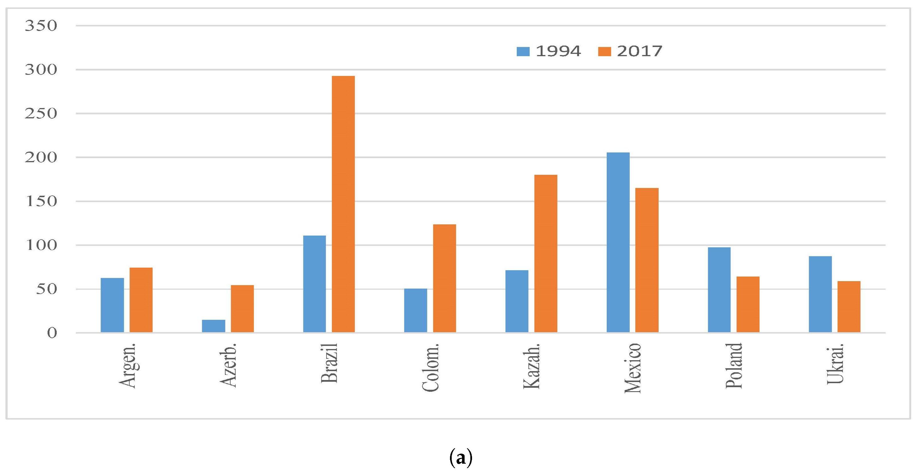
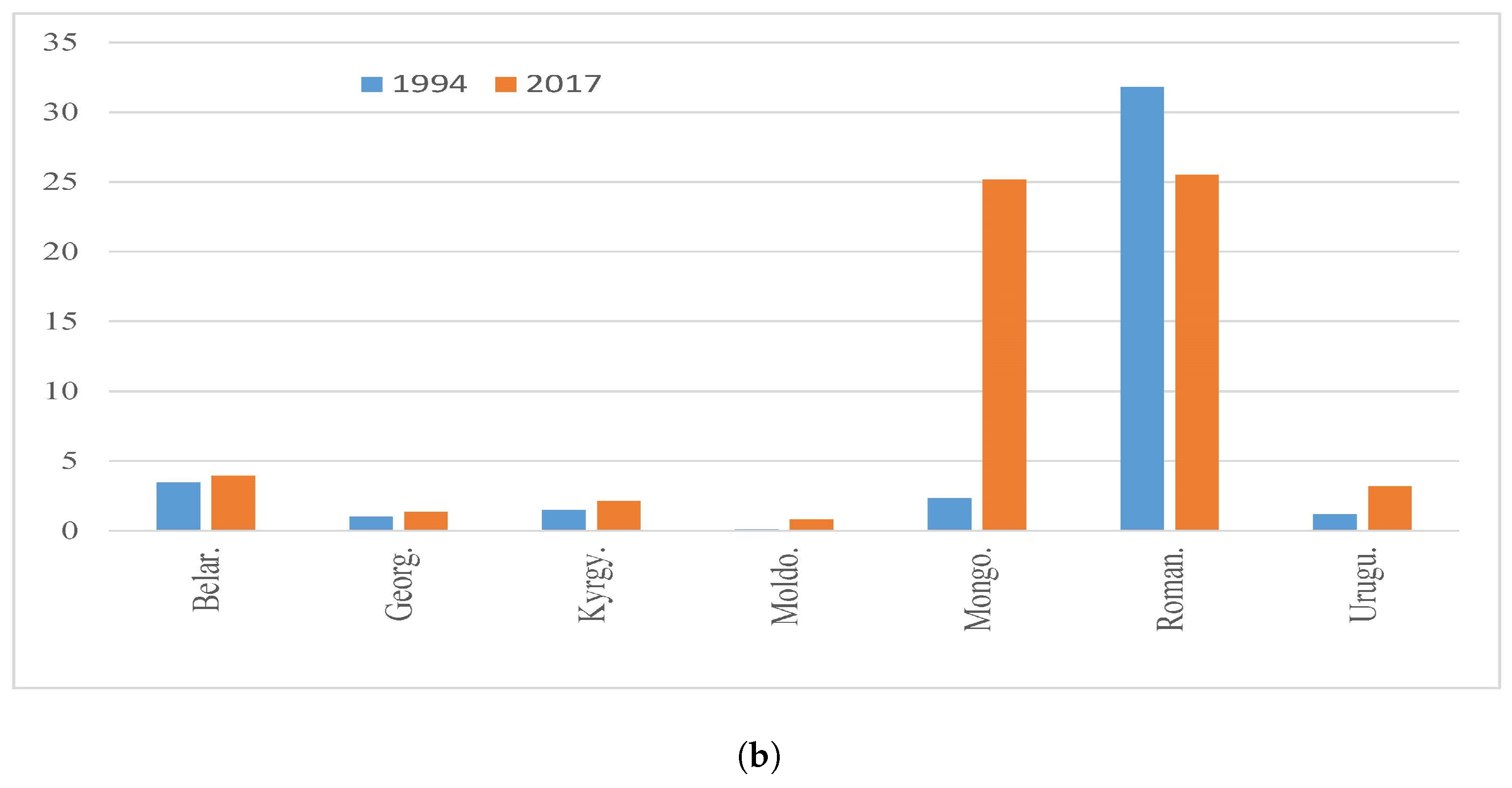
Annual data for 15 countries, representing several distinct geographic regions and political ideologies, covering the period 1994–2017, are examined. The energy variables were obtained from the International Energy Agency’s (IEA) country statistics. Energy production3 is the aggregate of production from all energy commodities, within a country. Total final consumption (TFC) accounts for the energy that is actually used by final consumers. The remaining variables were obtained from the World Development Indicators published by the World Bank (2019). Each country’s gross domestic product (GDP) is measured in millions of (constant 2010) US dollars and total population (Pop) in millions. Particular interest lies in the study of the financial variables (Fin), which include foreign direct investment (FDI), measured as net inflows as a percentage of GDP, and domestic credit to the private sector (DC), as a percentage of GDP.

Table 1. Country Level Summary Statistic for Select Variables, 1994–2017.

Country	Energy Production		FDI		Domestic Credit
	(Mtoe)		(Net Inflows as % of GDP)		(% of GDP)
	Mean	Std.dev.	Mean	Std.dev.	Mean	Std.dev
Argentina	78.431	6.243	−6495.158	4897.966	16.160	4.633
Azerbaijan	37.673	20.633	−522.127	1471.980	13.584	10.592
Belarus	3.648	0.265	945.158	960.939	19.545	10.330
Brazil	198.748	59.391	−33289.620	26943.480	45.543	14.580
Columbia	100.704	51.988	−5156.782	4014.216	37.033	9.246
Georgia	1.255	0.167	−717.764	543.751	23.422	18.308
Kazakhstan	119.203	41.847	−4944.888	4096.537	28.129	15.678
Kyrgyzstan	1.438	0.276	−222.732	269.451	10.962	6.026
Mexico	224.505	25.201	−18197.550	8514.846	22.179	6.723
Moldova	0.204 5	0.190	−189.443	161.000	22.411	10.374
Mongolia	8.164	7.690	−524.631	1597.347	29.640	19.180
Poland	78.042	11.293	−7678.208	3772.541	34.447	15.153
Romania	28.385	2.096	−3784.973	3413.045	22.304	11.907
Ukraine	77.806	7.560	−3258.292	3126.064	39.260	30.584
Uruguay	1.567	0.739	−823.480	1186.686	31.177	12.177
Note: The results are based on 24 observation, for each country.

presents summary statistics by country for both the energy and the financial development variables. On average, Mexico and Brazil have the highest level of energy production in the sample, although the maximum value observed by Columbia is above that observed for Brazil. Moldova is the smallest producer, with an average level of production just one sixth the size of the second lowest (Georgia). To get a sense of energy production across the sample of countries, Figure 2 presents the initial level of production (1994) and the final level (2017). The majority of the countries have experienced an increase in production over this time period, while Mexico, Poland, Ukraine, and Romania have experienced declining production. Brazil, as the largest economy in our sample, has the largest value of domestic credit. Given the recent political instability in the region, Ukraine has experience the largest variation in both economic performance and, subsequently, domestic credit. It is also noteworthy that Mongolia has experience significant variation in the level of domestic credit. This may be a function of requirements deriving from International Monetary Fund (IMF) lending programs. Of particular note, the average value of FDI is negative for this sample of countries.

3. Results

The panel unit root tests, with and without a (linear) trend, are presented in

Table 2. Results of the panel unit root tests.

Variable	LLC		IPS		Hadri
	No Trend	Trend	No Trend	Trend	No Trend	Trend
	t-statistic	t-statistic	t-statistic	t-statistic	t-statistic	t-statistic
Levels
Production	−2.066	−7.398 *	2.569	0.918	21.627 ***	8.873 ***
Energy Cons.	−2.132	−8.812 ***	2.911	−0.132	26.534 ***	9.205 ***
GDP	0.188	−8.102 *	6.109	0.487	27.868 ***	6.869 ***
Population	0.532	−13.352 ***	3.059	−4.322 ***	28.844 ***	22.789 ***
FDI	−7.130 **	−8.866	−1.799 **	−0.573	15.230 ***	5.502 ***
Dom. Credit	−4.388	−8.487	1.435	0.027	20.683 ***	11.238 ***
Differences
$\Delta$ Production	−13.789 ***	−17.335 ***	−8.424***	−8.147 ***	−2.054	−1.107
$\Delta$ Energy Cons.	−12.264 ***	−13.710 ***	−6.119***	−4.744 ***	0.461	5.042 ***
$\Delta$ GDP	−10.504 ***	−11.881 ***	−4.977 ***	−3.668 ***	0.874	9.0259 ***
$\Delta$ Population	−6.639 ***	−11.644 ***	−4.814 ***	−5.334 ***	20.109 ***	5.204 ***
$\Delta$ FDI	−15.955 ***	−16.480 ***	−10.895 ***	−8.551 ***	−1.999	1.479
$\Delta$ Dom. Credit	−12.121 ***	−13.241 ***	−6.275 ***	−4.702 ***	2.065	6.817 ***

Note: The results are based on 24 observation, for each country. ***, ** and * indicate statistical significance at the 1%, 5% and 10% levels, respectively.

. The three unit root tests provide strong evidence that, in levels, the variables contain a unit root. At the highest level of significance (1%), both the LLC and IPS test fail to reject the null hypothesis of no unit root, while the Hadri test consistently concludes (at the 1% level) that all variables are not stationary. The results of the unit root tests conducted on the first-differenced panels indicate that the variables are I(1). To be sure, the evidence from the Hadri test, particularly with a linear trend, provides us pause. However, the vast support provided by the LLC and IPS test results are sufficient to proceed to testing for cointegration and determine if a long run relationship exists.

Table 3. Results of the panel cointegration tests.

Panel A: Full model
	Model 1: FDI		Model 2: Dom. Credit
	No Time	Panel Specific	No Time	Panel Specific
Statistic	Effect	Time Trend	Effect	Time Trend
Panel Variance	−2.3652 ***	−3.8348 ***	−2.3547 ***	−3.8093 ***
Panel $\rho$	−0.6089	−0.3066	−0.2788	−0.3462
Panel PP	−6.0104 ***	−7.7412 ***	−5.8623 ***	−7.3394 ***
Panel ADF	−7.8199 ***	−8.7086 ***	−7.7769 ***	−8.5676 ***
Group $\rho$	−0.3049	0.7194	−0.0343	0.6626
Group PP	−8.4139 ***	−9.0598 ***	−9.3519 ***	−8.4418 ***
Group ADF	−10.5064 ***	−10.8590 ***	−11.0836 ***	−10.9443 ***
Panel B: Simplified Model
	Model 1: FDI		Model 2: Dom. Credit
	No Time	Panel Specific	No Time	Panel Specific
Statistic	Effect	Time Trend	Effect	Time Trend
Panel Variance	1.884 **	−1.921 **	1.996 **	−1.607 *
Panel $\rho$	−15.14 ***	−11.20 ***	−14.42 ***	−11.07 ***
Panel PP	−21.83 ***	−25.81 ***	−21.9 ***	−27.47 ***
Panel ADF	−18.45 ***	−23.17 ***	−19.16 ***	−22.54 ***
Group $\rho$	−12.05 ***	−8.012 ***	−11.77 ***	−7.804 ***
Group PP	−25.97 ***	−28.44 ***	−27.28 ***	−30.35 ***
Group ADF	−12.92 ***	−19.60 ***	−16.17 ***	−17.97 ***

Note: Panel B results are based on a test of only two variables-Production and Finance. ***, ** and * indicate statistical significance at the 1%, 5% and 10% levels, respectively.

provides the results of the cointegration test by Pedroni (2004), which consists of four within dimension (panel) test statistics and three between dimension (group) statistics. The majority of the results of the within dimension tests and the between dimension test suggest that there is strong evidence in favor of rejecting the null hypothesis of no cointegration, in each panel. The exceptions are both the within dimension panel $\rho$ and between dimension $\rho$ statistics. These results remain consistent when a panel specific time trend is also included and across both measures of financial development. The results of the cointegration tests suggest the presence of a long-run relationship among the variables in the model.

For robustness, and to focus the analysis, the cointegration test by Pedroni (2004) cointegration test was repeated for the simple model, which includes only energy production and a financial development variable. The results Part B of Table 3 support the hypothesis that a long run relationship exists, with the majority of the test statistics significant at the 1% level, when a panel specific time effect is included. Further support derives from the work of Wagner and Hlouskova (2010), who reported that, for small time samples $T\le 25$, the group ADF and panel ADF test have the best power properties, while the remaining tests are undersized and have low power. Specifically, the poor performance of the panel variance test and the group $\rho$ test has been documented. The results of the cointegration test by Westerlund (2005) are presented in

Table 4. Results of the Westerlund panel cointegration tests.

	Model 1: FDI		Model 2: Dom. Credit
	No Time	Panel Specific	No Time	Panel Specific
Statistic	Effect	Time Trend	Effect	Time Trend
$H_A:$Some panels are cointegrated
Variance Ratio	0.2977	−1.4627 *	−0.1789	−1.9690 **
$H_A:$All panels are cointegrated
Variance Ratio	−1.8338 *	−3.0399 ***	−1.9196 **	−3.2526 ***

Note: The H₀ is no cointegration. ***, ** and * indicate statistical significance at the 1%, 5% and 10% levels, respectively

. The empirical evidence indicates that the null hypothesis of no cointegration can be rejected in most cases, particularly in the case of the alternative hypothesis, where all panels are cointegrated.

The results of FMOLS on a per country basis, as well as for the panel as a whole, are reported in

Table 5. Panel FMOLS estimation.

	Model 1:		Model 2:
Variable	FDI	GDP	Dom. Credit	GDP
Argentina	20.99 (0.19)	−0.42 (−4.26)	−0.42 (−4.93) ***	−70.08 (−5.90) ***
Azerbaijan	686.90 (5.36) ***	1517.63 (42.9) ***	−0.33 (−13.6) ***	1636.0 (96.91) ***
Belarus	−30.06 (−2.21) ***	25.75 (9.98) ***	−0.00 (−0.6)	29.17 (12.7) ***
Brazil	94.65 (9.01) ***	24.15 (11.28) ***	−0.16 (−12.50) ***	25.29 (22.16) ***
Columbia	−543.22 (−0.61)	1451.05 (9.54) ***	1.58 (2.61) ***	964.06 (4.14) ***
Georgia	314.43 (9.03) ***	157.13 (7.01) ***	0.01 (1.74)	−58.40 (−0.70)
Kazakhstan	−913.34 (−4.12) ***	658.66 (6.61) ***	0.48 (14.15) ***	610.79 (11.03) ***
Kyrgyzstan	101.29 (1.70)	558.08 (7.80) ***	0.00 (0.29)	705.6 (2.70) ***
Mexico	−66.47 (−0.10)	−26.98 (−0.19)	−4.45 (−14.21) ***	−18.79 (−0.53)
Moldova	544.83 (10.9) ***	121.73 (6.97) ***	−0.02 (−32.08) ***	62.36 (8.35)
Mongolia	−773.80 (−8.01) ***	2482.62 (14.7) ***	−0.16 (−3.77)	2607.59 (10.62)
Poland	542.94 (5.85) ***	−133.70 (4.25) ***	−0.14 (−1.34)	182.63 (2.96)
Romania	155.91 (5.42) ***	97.74 (10.3) ***	0.04 (6.22) ***	54.63 (10.65) ***
Ukraine	632.87 (2.44) *	518.66 (10.9) ***	0.12 (29.4) ***	311.07 (62.57) ***
Uruguay	148.68 (9.55) ***	85.72 (15.07) ***	0.01 (21.74) ***	95.67 (46.87) ***
Group	61.11(11.5) ***	514.85(39.5) ***	−0.23(−1.78)	475.84(73.47) ***

Note: Figures in brackets are t-statistics. *** and * indicate statistical significance at the 1% and 10% levels, respectively. FDI and GDP were both rescaled by 1,000,000, while domestic credit remains as a percentage of GDP.

. The results demonstrate that, if FDI is the dependent variable of Equation (7), then energy production and FDI have a long run relationship in eleven of fifteen countries examined. For the panel, the coefficient of FDI is 61.1 with a t-statistic of 11.5, indicating the effect is positive and significant at the 1% level. From Model B in Table 3, energy production and domestic credit have a long run relationship in eleven of fifteen countries examined. The group statistic indicates that energy production and domestic credit and is negative, although insignificant.

The results of the bi-variate Dumitresu and Hurlin (2012) panel Granger causality tests are presented in

Table 6. Short run relationship based on granger causality results.

Part A: FDI
Variables	$\mathbf{\Delta }$Production		$\mathbf{\Delta }$Energy Cons.		$\mathbf{\Delta }$Pop.		$\mathbf{\Delta }$GDP		$\mathbf{\Delta }$FDI
	t-stat	p-Value	t-stat	p-Value	t-stat	p-Value	t-stat	p-Value	t-stat	p-Value
$\Delta$ Production	.	.	1.195	0.232	13.170 ***	0.000	2.369 **	0.018	1.442	0.149
$\Delta$ Energy Cons.	1.151	0.250	.	.	6.234 ***	0.000	0.002	0.998	4.583 ***	0.000
$\Delta$ Pop.	5.389 ***	0.000	8.257 ***	0.000	.	.	8.602 ***	0.000	3.400 ***	0.001
$\Delta$ GDP	1.050	0.294	2.018 **	0.044	3.967 ***	0.000	.	.	0.610	0.542
$\Delta$ FDI	13.749 ***	0.000	3.225 ***	0.001	−1.284	0.199	4.898 ***	0.000	.	.
Part B:Domestic Credit
Variables	$\mathbf{\Delta }$Production		$\mathbf{\Delta }$Energy Cons.		$\mathbf{\Delta }$Pop.		$\mathbf{\Delta }$GDP		$\mathbf{\Delta }$Dom. Credit
	t-stat	p-Value	t-stat	p-Value	t-stat	p-Value	t-stat	p-Value	t-stat	p-Value
$\Delta$ Production	.	.	1.195	0.232	13.17 ***	0.000	1.050	0.294	0.434	0.664
$\Delta$ Energy Cons.	1.322	0.186	.	.	4.974 ***	0.000	−0.033	0.974	1.304	0.192
$\Delta$ Pop.	5.389 ***	0.000	8.257 ***	0.000	.	.	8.602 ***	0.000	1.300	0.194
$\Delta$ GDP	2.369	0.017	2.018 **	0.044	3.967***	0.00	.	.	0.553	0.581
$\Delta$ Dom. Credit	−0.971	0.332	4.113***	0.000	−0.036 ***	0.006	3.633 ***	0.000	.	.

Note: Two lags were utilized for each of the tests. *** and ** indicate statistical significance at the 1% and 5% levels, respectively.

. Given the size of the panel ($N=15$ and $T=24$), the $\overline{Z}$ test statistics are examined, while the lag length was determined by AIC criteria. The results in Part A focus on FDI as the financial development variable and indicate that changes in production cause changes in FDI, although the reverse is not true. We infer from the results that foreign capital is attracted to the economy by increasing levels of energy production, rather than energy production relying on foreign capital as a source of funding. The majority of the remaining results are in line with expectations. Bi-directional causality is observed between population and GDP, as well as population and energy consumption. Unilateral causation is observed from population to energy production and GDP to FDI. The results of Model 2, presented in Part B of Table 6, demonstrate no causal relationship between domestic credit and energy production. The implication of this result is that internal sources of funding do not appear to be relevant for the domestic production of energy resources. Furthermore, domestic credit does not Granger cause any of the remaining variables in the model. In essences, there is a short run relationship between energy production and FDI, but not energy production and domestic credit, in this sample of countries.

4. Discussion

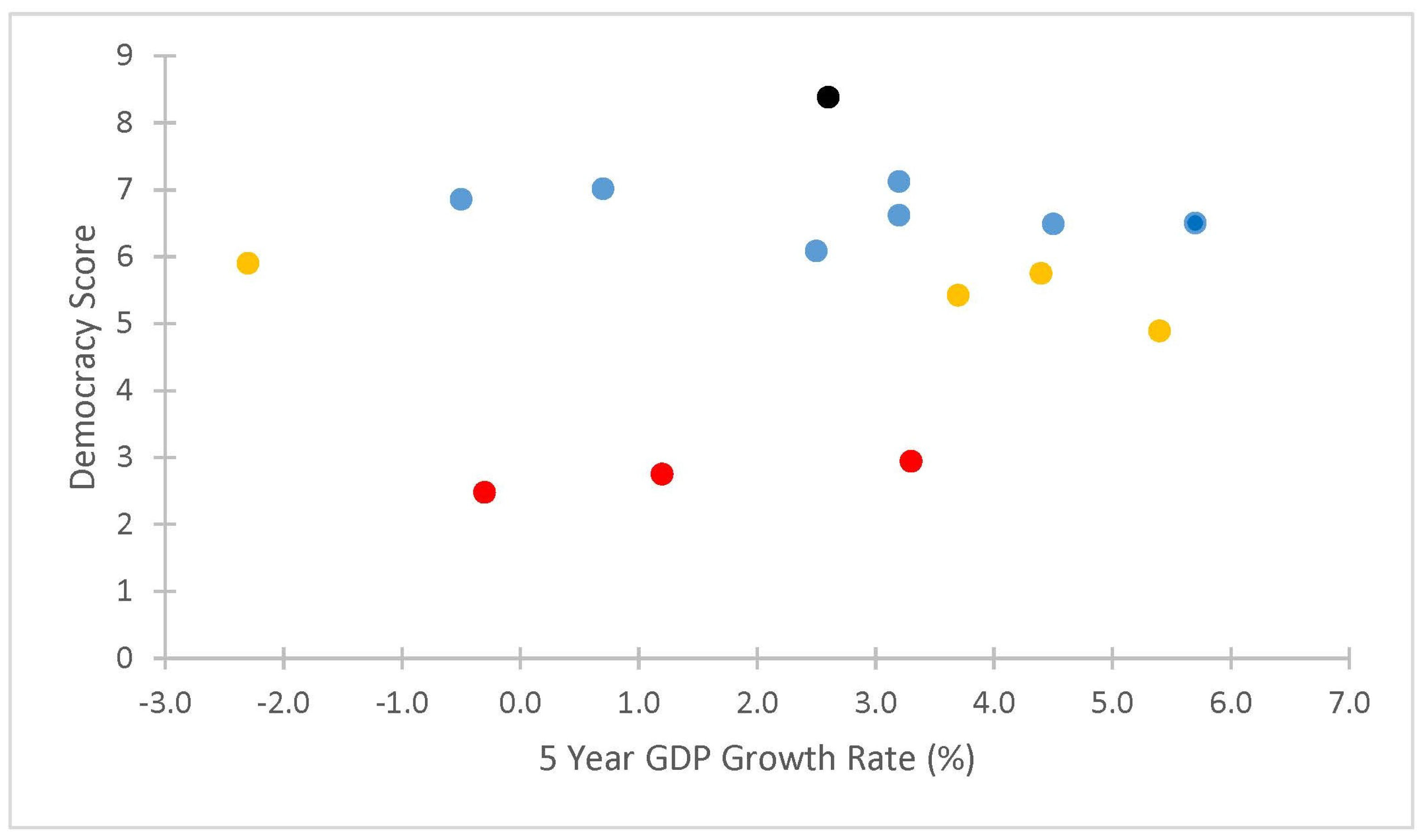
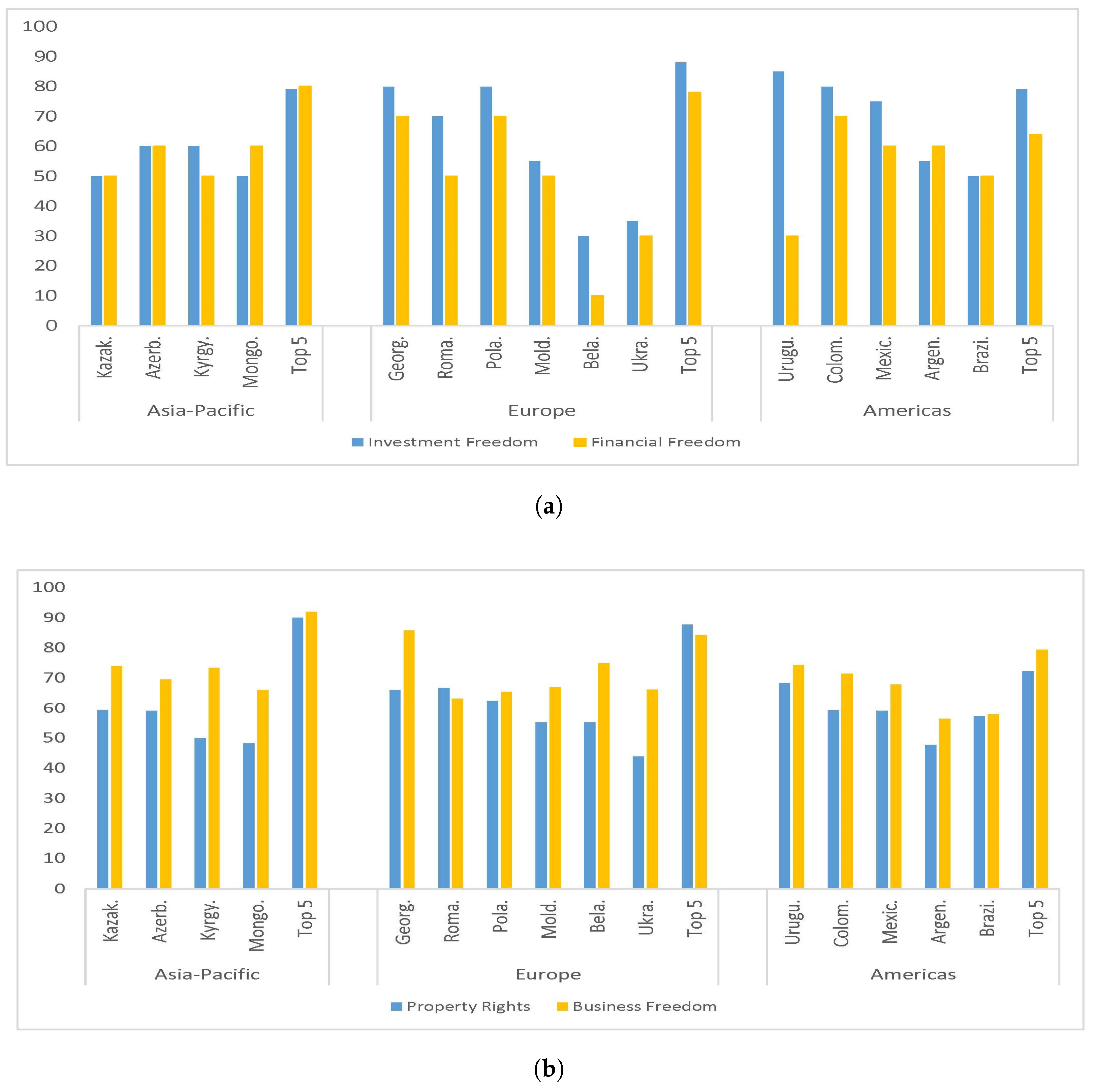
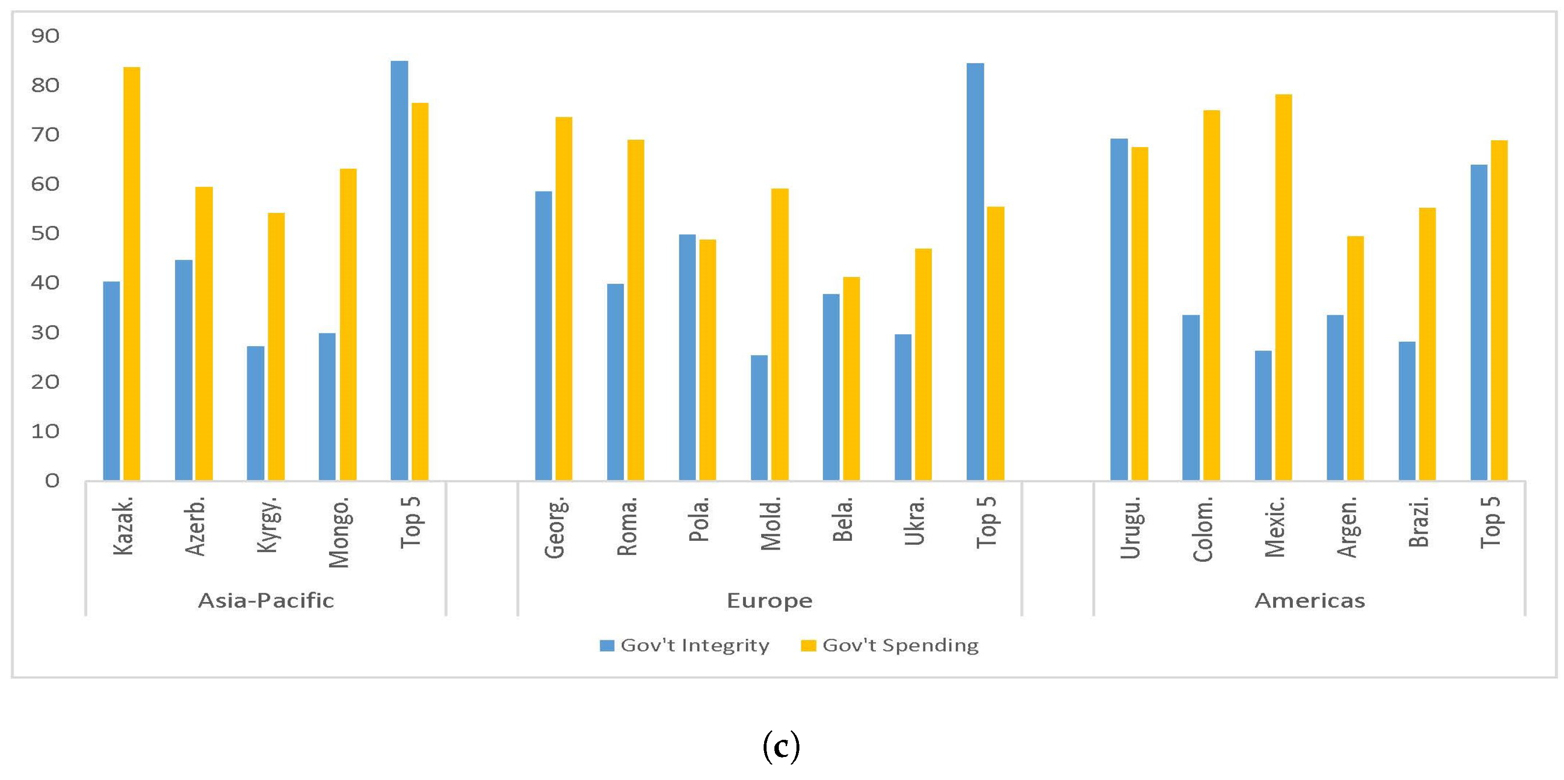
Before drawing additional inferences, we further examine the characteristics of the sample countries in this study. The sample draws from the population of emerging economics, with a cross-section of states in various stages of development. Using data from The Economist (2020), Figure 3 demonstrates the current level of democracy, for this sample of countries. We note that only Uruguay is listed as a full democracy, while the rest range from flawed democracy (blue) to authoritarian regimes (red). The remaining countries are considered to be hybrids, which have serious weaknesses in the functioning of government and widespread corruption. According to the Heritage Foundation (2020), the level of prosperity a country experiences is positively related to the economic freedom amassed by that country. The Heritage Foundation constructs an annual ranking for nearly every country, based upon the country’s economic freedom. The index is an aggregate across a number of subcategories consisting of business, trade, property rights, and governance. Based on the 2019 edition of the Index of Economic Freedom, 6 of our 15 countries fall in the lowest quartile of world rankings, and only Georgia lies within the top 40 countries ranked by the foundation. Across this sample, only Brazil (57.9) and Argentina (56.4) have values less than 60 out of a possible 100. Separated by geographic region, Figure 4 presents six component of the Index of Economic Freedom, for each of the countries, as well as the average of the Top 5 countries for each of the geographic regions. In Figure 4a, only Uruguay and Colombia have investment freedom above the average of the Top 5, although, in the Americas, the variance seems much lower than that of Europe. Belarus has only 34% of the investment freedom experienced by the Top 5 countries, with financial freedom even lower, at only 13% of the Top 5. In Figure 4b, this sample experiences accentuated levels of disenfranchisement when it comes to property rights, and the business freedom is considerably lower in this sample of countries. Only Georgia is above the average of the Top 5 in any region. The Heritage Foundation has specifically recognized that Georgia has experienced significant increase in its Economic Freedom since its first year on the index. Figure 4c examines two measures that pertain to the government of the country. Government integrity is particularity low in our sample of countries, highlighting the high degree of corruption and absence of the rule of law. The final variable, government spending, demonstrates that many of the countries experience an enlarged level of government expenditures, as a proportion of GDP, relative to the Top 5 ’free’ countries in that region.

Understanding that the sample contains undemocratic countries with lower property rights and restricted access to investments allows our results to be put into context. The results of the Granger causality tests indicate that a short run relationship between energy production and FDI exists, but not energy production and domestic credit. This aligns with the characteristics of the sample; with lower levels of property rights and less investment freedom domestically, it falls to the government or foreign firms (via FDI) to provide the necessary capital to extract and produce energy. This also accords with the work of Dunkerley (1995), who examined energy sector financing, in emerging countries. They argued the provision of energy supplies is essential for economic growth, and noted that the role of private capital has been dominated by the public sector.

Based on the results of the panel cointegration tests, a long-term relationship between the variables is confirmed, at least in one direction. The parameters of the long-term relationship, estimated using the panel FMOLS method, demonstrate a significant relationship with FDI, for many of the countries in our sample. The panel Granger causality test results demonstrate a uni-directional relationship from energy production to FDI. The results are similar to those of Shan and Morris (2002), with the empirical results failing to provide support for the hypothesis that financial development “leads” energy production, and supporting the hypothesis that the link between financial development and energy production may be country specific. Indeed, as in Taivan (2016), the conclusions herein may be attributed to a wide variation in the policies governing the financial sector and other institutional factors.

Following North (1991), economists are acutely aware of the essential role of institutions to create efficient markets, which can facilitate the growth of the economy. Germane to this sample, one must consider that the majority of economies have experienced a momentous structural change in economic institutions over the time period studied. The underdevelopment of the requisite financial institutions would inhibit the coordination of domestic savings and domestic borrowing, thus limiting domestic funding of large-scale capital projects associated with primary energy production.

The demonstrated importance of the energy sector and its role in the economy means that an understanding of the factors affecting the development of this sector are crucial for developing economies. This point may be particularly poignant for an economy with a large endowment of energy commodities. Additionally, reliable energy supplies are of demonstrated importance to the development of a country [(Dunkerley 1995; Koçak and Şarkgüneşi 2017)]. While the results demonstrate that foreign capital is attracted to the economy and increasing levels of energy production, undoubtedly, a strengthening of the domestic financial market along with propriety rights would benefit these emerging economies.

5. Conclusions

The ability to meet the continual rise in global energy demand requires further investment in capital intensive projects. While such large scale investments is beneficial to an economy, it requires significant financing, which can be especially difficult to obtain in emerging economies. Therefore, understanding the relationship between energy production and financial development is paramount for those developing economies endowed with significant energy resources. The results of the FMOLS estimation provide evidence of a long run relationship for 11 of the 15 emerging economies studied. The causal relationship from energy production to FDI is an important link for policy makers to understand. It should be understood that the designing and implementation of energy policy can affect the inflow of FDI and alter the rate of economic growth. The lack of a causal relationship from FDI to energy production is similar to the findings of Shan and Morris (2002). The authors reported empirical results which fail to provide support for the hypothesis that financial development “leads” energy production and support the hypothesis that the link between financial development and energy production may be country specific. Indeed, as in Taivan (2016), the conclusions herein may be attributed to a wide variation in the policies governing the financial sector and other institutional factors. Our results also highlight the dominant role FDI has relative to domestic credit, in this sample of 15 countries. This result may present a significant challenge to the countries in our sample, given the authoritarian nature of several regimes. Relinquishing control of what is often considered a strategic sector of the economy could be difficult to undertake, even with the additional benefit of increased inflows of FDI.

References

- Belousov, Lev, and Alexei Vlasov. 2010. The post-Soviet space: A transition period. Transition Studies Review 17: 108–22. [Google Scholar] [CrossRef]
- Chiu, Yi-Bin, and Chien-Chiang Lee. 2020. Effects of financial development on energy consumption: The role of country risks. Energy Economics 90: 104833. [Google Scholar] [CrossRef]
- Christopoulos, Dimitris K., and Efthymios G. Tsionas. 2004. Financial development and economic growth: Evidence from panel unit root and cointegration tests. Journal of Development Economics 73: 55–74. [Google Scholar] [CrossRef]
- Cust, James, and Torfinn Harding. 2000. Institutions and the location of oil exploration. Journal of the European Economic Association 18: 1321–50. [Google Scholar] [CrossRef]
- Demetriades, Panicos, and Khaled A. Hussein. 1996. Does financial development cause economic growth? time-series evidence from 16 countries. Journal of Development Economics 51: 378–411. [Google Scholar] [CrossRef]
- Dowling, Malcolm, and Ganeshan Wignaraja. 2007. Central asia after fifteen years of transition: Growth, regional cooperation, and policy choices. Asia-Pacific Development Journal 13: 113–44. [Google Scholar] [CrossRef]
- Dumitresu, Elena-Ivona, and Christophe Hurlin. 2012. Testing for granger causality in heterogenous panels. Economic Modelling 29: 1450–60. [Google Scholar] [CrossRef] [Green Version]
- Dunkerley, Joy. 1995. Financing the energy sector in developing countries: Context and overview. Energy Policy 23: 929–39. [Google Scholar] [CrossRef]
- Energy Information Administration. 2015. World Shale Resource Assessment. Available online: www.eia.gov (accessed on 20 January 2021).
- Energy Information Administration. 2019. Belarus energy profile. Available online: www.eia.gov (accessed on 10 December 2020).
- Energy Information Administration. 2020. Argentina Energy Analysis. Available online: www.eia.gov (accessed on 10 December 2020).
- Ghedrovici, Olesea, and Nikolai Ostapenko. 2013. The glaring socioeconomic meltdown in post-Soviet ukraine, moldova, and belarus: A distorted mindset in search of a way out. International Journal of Business and Social Research 3: 202–11. [Google Scholar]
- Hadri, Kaddour. 2000. Testing for stationarity in heterogeneous panel data. Econometrics Journal 3: 148–61. [Google Scholar] [CrossRef]
- Heritage Foundation. 2020. 2019 Index of Economic Freedom. Washington, DC: Heritage Foundation. [Google Scholar]
- Im, Kyung S., M. Hashem Pesaran, and Yongcheol Shin. 2003. Testing for unit root in heterogeneous panels. Journal of Econometrics 115: 53–74. [Google Scholar] [CrossRef]
- International Energy Agency. 2019. Data and Statistics Website Data Browser. Available online: www.iea.org (accessed on 10 January 2020).
- Koçak, Emrah, and Aykut Şarkgüneşi. 2017. The renewable energy and economic growth nexus in black sea and balkan countries. Energy Policy 100: 51–57. [Google Scholar] [CrossRef]
- Kwiatkowski, Denis, Peter C. B. Phillips, Peter Schmidt, and Yongcheol Shin. 1992. Testing the null hypothesis of stationarity against the alternative of a unit root. Journal of Econometrics 54: 159–78. [Google Scholar] [CrossRef]
- Lee, Chien-Chang, and Chun-Ping Chang. 2009. Fdi, financial development, and economic growth: International evidence. Journal of Applied Economics 12: 249–71. [Google Scholar] [CrossRef]
- Levin, Andrew, Chien-Fu Lin, and Chia-Shang James Chu. 2002. Unit root tests in panel data: Asymptotic and finite sample properties. Journal of Econometrics 108: 1–24. [Google Scholar] [CrossRef]
- Levine, Ross, and Sara Zervos. 1998. Stock market, banks, and economic growth. American Economic Review 88: 537–58. [Google Scholar]
- McKinnon, Ronald I. 1973. Money and Capital in Economic Development. Washington, DC: The Brookings Institution. [Google Scholar]
- North, Douglas. C. 1991. Institutions. Journal of Economic Perspectives 5: 97–112. [Google Scholar] [CrossRef]
- Oil and Energy Trends. 2019. Kazakhstan Rising output and a change of leadership. Oil and Energy Trends 44: 3–5. [Google Scholar] [CrossRef]
- Pedroni, Peter. 1999. Critical values for cointegration tests in heterogeneous panels with multiple regressors. Oxford Bulletin of Economics and Statistics 61: 653–70. [Google Scholar] [CrossRef]
- Pedroni, Peter. 2000. Fully modified ols for heterogeneous cointegrated panels. Advances in Econometrics 15: 93–130. [Google Scholar]
- Pedroni, Peter. 2004. Panel cointegration: Asymptotic and finite sample properties of pooled time series tests with an application to the ppp hypothesis. Econometric Theory 20: 597–25. [Google Scholar] [CrossRef] [Green Version]
- Sadorsky, Perry. 2010. The impact of financial development on energy consumption in emerging economies. Energy Policy 38: 2528–35. [Google Scholar] [CrossRef]
- Schumpeter, Joseph. A. 1911. The Theory of Economic Development. Cambridge: Harvard University Press. [Google Scholar]
- Shan, Jordan Z., and Alan Morris. 2002. Does financial development ‘lead’ economic growth? International Review of Applied Economics 16: 153–68. [Google Scholar] [CrossRef]
- Shaw, Edward Stone. 1973. Financial Deepening in Economic Development. New York: Oxford University Press. [Google Scholar]
- Shujing, Yue, Rou Lu, Yongshang Shen, and Hongtao Chen. 2019. How does financial development affect energy consumption? evidence from 21 transitional countries. Energy Policy 133: 253–62. [Google Scholar]
- Taivan, Ariuna. 2016. The causality between financial development and economic growth: Case of asian economies. Economics Bulletin 36: 1071–82. [Google Scholar]
- Taivan, Ariuna, and Gibson Nene. 2016. Financial development and economic growth: Evidence from southern african development community countries. Journal of Developing Areas 50: 81–95. [Google Scholar] [CrossRef]
- The Economist. 2020. The Democracy Index 2019 Report. Technical Report. London: The Economist Intelligence Unit. [Google Scholar]
- Wagner, Martin, and Jaroslava Hlouskova. 2010. The performance of panel cointegration methods: Results from a large scale simulation study. Economic Review 29: 182–223. [Google Scholar] [CrossRef]
- Westerlund, Joakim. 2005. New simple tests for panel cointegration. econometric reviews. Econometric Reviews 24: 297–316. [Google Scholar] [CrossRef]
- World Bank. 2017. Press Release: World Bank Group announcements at One Planet Summit. Washington, DC: World Bank Press. [Google Scholar]
- World Bank. 2019. World Development Indicators. Washington, DC: World Bank Press. [Google Scholar]